Three dimensional numerical simulations of acoustic wave field in the upper convection zone of the Sun

Abstract

Results of numerical 3D simulations of propagation of acoustic waves inside the Sun are presented. A linear 3D code which utilizes realistic OPAL equation of state was developed by authors. Modified convectively stable standard solar model with smoothly joined chromosphere was used as a background model. High order dispersion relation preserving numerical scheme was used to calculate spatial derivatives. The top non-reflecting boundary condition established in the chromosphere absorbs waves with frequencies greater than the acoustic cut-off frequency which pass to the chromosphere, simulating a realistic situation. The acoustic power spectra obtained from the wave field generated by sources randomly distributed below the photosphere are in good agreement with observations. The influence of the height of the top boundary on results of simulation was studied. It was shown that the energy leakage through the acoustic potential barrier damps all modes uniformly and does not change the shape of the acoustic spectrum. So the height of the top boundary can be used for controlling a damping rate without distortion of the acoustic spectrum. The developed simulations provide an important tool for testing local helioseismology.

1 Introduction

Solar 5-min. oscillations are excited by turbulent convection (downdrafts) in subsurface layers of the Sun. These oscillations consist of acoustic and surface gravity waves with frequencies in the range of 2$\div$8 mHz and in a wide range of wave numbers. The observed oscillations can be used for reconstruction of internal structure of the Sun by methods of helioseismology. There are several methods of investigation of the interaction of traveling acoustic waves with small perturbations to the background state. One of them is the time-distance approach (Duvall et al., 1993; Kosovichev, 1996). The key concept of this method is measuring and inversion of wave travel times. Propagation of acoustic waves in this approach is calculated using various approximations to the wave equations, such as the ray theory or first Born approximation (Kosovichev & Duvall, 1997; Kosovichev et al., 2000; Jensen et al., 2001; Couvidat et al., 2004, 2006). These approximations have been tested using simple models for point sources (e.g. Birch et al. (2001); Birch & Felder (2004)), but not for realistic solar conditions, e.g. realistic stratification and random excitation sources. Such tests, which require direct numerical simulations, are extremely important for validating the inferences from time-distance helioseismology and other local helioseismology methods.

There are two main directions in numerical simulations of solar oscillations and waves. The first one is to use realistic non-linear simulations of solar convection. In such simulations, the waves are naturally excited by convective motions. These simulations reproduce quite well the solar oscillation spectrum Stein et al. (2004), and have been used for testing time-distance helioseismology Georgobiani et al. (2006). The second approach is based on linearized Euler equations describing wave propagation for a given background state. The background state can be taken from non-linear numerical simulations or by perturbing the standard solar model. In this paper, we describe a numerical method and initial simulation results developed for the second approach.

We developed a 3D code which utilizes a realistic physics and accurately simulates reflection of acoustic waves from the top boundary. A realistic equation of state which takes into account partial ionizations and various corrections is used. The equation of state was calculated by interpolation of the OPAL tables. In Section 2.1 we give a detailed description of the underlying physics. The main attention is paid to developing a consistent procedure for obtaining a convectively stable background model and establishing realistic top boundary conditions based on the Perfectly Match Layer (PML) method. In Section 2.2 we describe a semi-discrete numerical scheme of high order which preserves dispersion relations of the continuous problem. The main attention is paid to developing stable high-order numerical boundary conditions consistent with the finite-difference scheme, in which the dispersion relation is preserved for the inner mesh points of the computational domain. In Section 3, we compare the numerical and analytical solutions of various 1D test problems with an isothermal background model to validate the code, investigate accuracy of the numerical scheme, and the non-reflecting boundary conditions in a gravitationally stratified medium. In Section 4, we present results of numerical three dimensional simulations of acoustic wave field for a standard solar background model. We used different types of single or multiple acoustic sources: z-component of force or pressure, point or distributed with different time dependence. The main goals are to study properties of solar waves for various excitation sources and generate artificial wave fields for testing accuracy of the Born and ray approximations and local helioseismic diagnostics of the solar interior, currently used for SOHO/MDI and GONG data. The results of this testing will be presenting in future papers. The numerical simulations are carried out on parallel supercomputers at NASA Ames Research center.

2 Code description

2.1 Physical background

The propagation of adiabatic acoustic waves below the solar photosphere is described by the following system of linearized Euler equations:

$$\begin{array}[]{l}\displaystyle\frac{\partial\rho^{\prime}}{\partial t}+\frac{\partial}{\partial x}(\rho_{0}u^{\prime})+\frac{\partial}{\partial y}(\rho_{0}v^{\prime})+\frac{\partial}{\partial z}(\rho_{0}w^{\prime})=0\vspace{5pt}\\ \displaystyle\frac{\partial}{\partial t}(\rho_{0}u^{\prime})+\frac{\partial p^{\prime}}{\partial x}=0\vspace{5pt}\\ \displaystyle\frac{\partial}{\partial t}(\rho_{0}v^{\prime})+\frac{\partial p^{\prime}}{\partial y}=0\vspace{5pt}\\ \displaystyle\frac{\partial}{\partial t}(\rho_{0}w^{\prime})+\frac{\partial p^{\prime}}{\partial z}=-g_{0}\rho^{\prime},\end{array}$$ (1)

where $u^{\prime},v^{\prime},w^{\prime}$ are the perturbations of $x,y,z$ velocity components, $\rho^{\prime}$ and $p^{\prime}$ are the density and pressure perturbations correspondingly. Quantities with subscript 0 such as the pressure $p_{0}$, the density $\rho_{0}$, and the gravitational acceleration $g_{0}$ correspond to the background reference model and depend only on radius. Christensen-Dalsgaard’s standard solar model S (Christensen-Dalsgaard et al., 1996) with smoothly joined chromosphere provided by Vernazza et al. (1976) was chosen as such a model. To close the system we use an adiabatic relation between Eulerian variations of pressure $p^{\prime}$ and density $\rho^{\prime}$

$$p^{\prime}=a_{0}^{2}\rho^{\prime}-a_{0}^{2}\frac{N_{0}^{2}}{g_{0}}(\rho_{0}\xi_{z}),$$ (2)

where $a_{0}^{2}=\Gamma_{1}p_{0}/\rho_{0}$ is the square of sound speed, $\Gamma_{1}=(\partial\log p/\partial\log\rho)_{ad}$ is the adiabatic exponent, $N_{0}$ is the Brunt-Väisälä frequency, $\xi_{z}$ is the vertical displacement. So, from the background model we need only profiles of the sound speed and Brunt-Väisälä frequency.

The background state is convectively unstable, especially just below the photosphere, where the temperature gradient is super-adiabatic and convective motions are very intense and turbulent. This leads to the instability of the solution of linear system (1). Convection instability is developed on a time scale of 30-40 minutes of solar time. Simulation of the acoustic spectrum of solar oscillations needs to perform calculations on a time interval of 5-8 hours of solar time, and this instability will badly distort the result. To make the background model stable against convection we slightly modified profiles of pressure and density in a thin (500 km in depth) super-adiabatic layer just below the photosphere. The condition for stability against convection requires that the square of Brunt-Väisälä frequency has to be positive

$$N^{2}(r)=g\left(\frac{1}{\Gamma_{1}}\frac{\mbox{d}\log p}{\mbox{d}r}-\frac{\mbox{d}\log\rho}{\mbox{d}r}\right)>0,$$ (3)

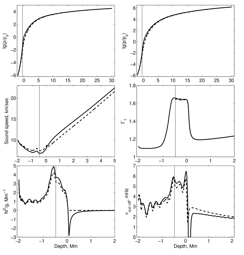
Figure 1: Vertical profiles of the density, pressure, sound speed, adiabatic exponent, Brunt-Väisälä frequency, and acoustic cut-off frequency. Solid curves represent profiles for the standard solar model with smoothly joined chromosphere, dashed ones show the profiles of the convectively stable modified model.

where $r$ is the distance from the center of the Sun. The profile of $N^{2}$ near the solar surface is shown in the bottom left pane of Figure 1 by the solid line. If we replace negative values by zero (or small positive) value we guarantee a stability of the modified model against convection. Now we can recalculate the pressure and density from the modified profile of $N_{mod}^{2}$. Combining equation (3) with the condition of hydrostatic equilibrium, we get the following boundary value problem for $p$ and $\rho$:

$$\begin{array}[]{l}\displaystyle\frac{1}{\rho}\frac{\mbox{d}\rho}{\mbox{d}z}=-\frac{g}{c^{2}}-\alpha\frac{N_{mod}^{2}}{g},\\[9.0pt] \displaystyle\frac{\mbox{d}p}{\mbox{d}z}=-\rho g,\\[7.0pt] 0\leq z\leq L,\quad\rho(0)=\rho_{0}(0),\quad\rho(L)=\rho_{0}(L),\quad p(L)=p_{0}(L),\end{array}$$ (4)

where $L$ is the depth of the computational domain, $z$ is the vertical coordinate which is counted off from the bottom of the domain. We introduced a free parameter $\alpha$ that has to be determined, to make the modified model closer to the original one. We established boundary conditions for the system (4) setting the density at the top and bottom boundaries equal to solar values. Parameter $\alpha$ does not change the condition of convective stability if it remains positive. Introducing of an additional parameter permits us to establish yet another boundary condition and fix the pressure at the top boundary. So the recipe to build a convectively stable background model close to the standard one is the following. We smoothly join the density profiles of the standard solar model and the chromosphere, obtain the pressure profile from the condition of hydrostatic equilibrium, calculate square of the modified Brunt-Väisälä frequency profile $N^{2}_{mod}$, replacing negative values by a zero or small positive value, and substitute it into the right hand side of (4). Parameter $\alpha$, profiles of density and pressure of the modified convectively stable model are obtained as a solution of the eigenvalue problem (4). The profile of $\Gamma_{1}$, needed for the sound speed profile, is found from the realistic OPAL equation of state (Rogers et al., 1996). Vertical profiles of pressure $p_{0}$, density $\rho_{0}$, sound speed $a_{0}$, square of Brunt-Väisälä frequency $N^{2}$, adiabatic exponent $\Gamma_{1}$, and acoustic cut-off frequency

$$\omega_{c}^{2}=\frac{a_{0}^{2}}{4H^{2}}\left(1-2\frac{\mbox{d}H}{\mbox{d}r}\right),\quad H^{-1}=-\frac{\mbox{d}\log\rho_{0}}{\mbox{d}r}$$ (5)

for both models (standard with joined chromosphere and modified convectively stable) are shown in Figure 1. The depth of the domain from the photosphere equals 30 Mm, the height of the chromosphere equals 2 Mm, $\alpha=0.861$. The dashed curves represent profiles in the convectively stable model, the solid lines show profiles of the standard solar model. The thin vertical line marks the position of the fitting point of the chromosphere and the standard solar model. The background model, obtained with the procedure described above, is convectively stable and self-consistent.

2.2 Numerical algorithm

The system (1) is written in a conservative form

$$\frac{\partial\mbox{\boldmath$q$}}{\partial t}+\frac{\partial\mbox{\boldmath$F$}(\mbox{\boldmath$q$})}{\partial x}+\frac{\partial\mbox{\boldmath$G$}(\mbox{\boldmath$q$})}{\partial y}+\frac{\partial\mbox{\boldmath$H$}(\mbox{\boldmath$q$})}{\partial z}=\mbox{\boldmath$S$}(\mbox{\boldmath$q$},t),$$ (6)

where $\mbox{\boldmath$q$}=(\rho^{\prime},\rho_{0}u^{\prime},\rho_{0}v^{\prime},\rho_{0}w^{\prime})^{T}$ is the vector of independent variables, $\mbox{\boldmath$S$}(\mbox{\boldmath$q$},t)$ is the source term containing the gravity term and acoustic sources which depend on time explicitly. The source term does not contain spatial derivatives. Explicit expressions for components of vectors $F$, $G$, and $H$ can be easily found from the system (1). We used a semi-discrete numerical scheme. In semi-discrete approach the space and time discretization processes are separated. First the spatial discretization is performed, leaving the problem continuous in time. The spatial derivatives have been approximated by the finite difference method reducing the system of partial differential equations to the system of ordinary differential equations

$$\begin{array}[]{lcl}\displaystyle\frac{\mbox{d}\mbox{\boldmath$q$}_{ikj}}{\mbox{d}t}&=&L_{ikj}(\mbox{\boldmath$q$},t),\\[7.0pt] \displaystyle L_{ikj}(\mbox{\boldmath$q$},t)&=&\displaystyle-\frac{1}{\Delta x}\sum_{l=-3}^{3}a_{l}\mbox{\boldmath$F$}_{i,k,j+l}-\frac{1}{\Delta y}\sum_{l=-3}^{3}a_{l}\mbox{\boldmath$G$}_{i,k+l,j}\\[7.0pt] &-&\displaystyle\frac{1}{\Delta z}\sum_{l=-3}^{3}a_{l}\mbox{\boldmath$H$}_{i+l,k,j}+\mbox{\boldmath$S$}_{ikj}(t)\end{array}$$ (7)

which can be solved by any stable time advancing method. We used four stage, 3rd order strong-stability-preserving Runge-Kutta method (Shu, 2002) with Courant number $c=2$:

$$\begin{array}[]{l}\displaystyle\mbox{\boldmath$q$}^{(1)}=\mbox{\boldmath$q$}^{(n)}+\frac{1}{2}\Delta t\,L(\mbox{\boldmath$q$}^{(n)},t^{n}),\\[7.0pt] \displaystyle\mbox{\boldmath$q$}^{(2)}=\mbox{\boldmath$q$}^{(1)}+\frac{1}{2}\Delta t\,L(\mbox{\boldmath$q$}^{(1)},t^{n}+\frac{1}{2}\Delta t),\\[7.0pt] \displaystyle\mbox{\boldmath$q$}^{(3)}=\frac{2}{3}\mbox{\boldmath$q$}^{(n)}+\frac{1}{3}\mbox{\boldmath$q$}^{(2)}+\frac{1}{6}\Delta t\,L(\mbox{\boldmath$q$}^{(2)},t^{n}+\Delta t),\\[7.0pt] \displaystyle\mbox{\boldmath$q$}^{(n+1)}=\mbox{\boldmath$q$}^{(3)}+\frac{1}{2}\Delta t\,L(\mbox{\boldmath$q$}^{(3)},t^{n}+\frac{1}{2}\Delta t).\end{array}$$ (8)

The source term $\mbox{\boldmath$S$}(\mbox{\boldmath$q$},t)$ which depends on time explicitly does not require a special treatment.

High-order dispersion-relation-preserving (DRP) scheme developed by Tam & Webb (1993) was used for spatial discretization. Coefficients $a_{l}$ of the finite difference scheme

$$\left.\frac{\partial f}{\partial x}\right|_{j}\simeq\frac{1}{\Delta x}\sum_{l=-3}^{3}a_{l}f_{j+l}=\frac{1}{\Delta x}\sum_{l=-3}^{3}a_{l}f(x_{j}+l\Delta x)$$ (9)

are chosen from the requirement that the difference between Fourier transform of the numerical scheme and Fourier transform of the spatial derivative has to be minimal. Taking the Fourier transform of both sides of (9) one can get the effective wave number $k_{eff}$ of the Fourier transform of the numerical scheme (9)

$$k_{eff}=-\frac{i}{\Delta x}\sum_{l=-3}^{3}a_{l}e^{ilk\Delta x}.$$ (10)

An assumption that the integral error $E$ of Fourier transform of the finite difference scheme (9) is minimal for waves with wavelength $\lambda\geq 4\Delta x$ leads to the following equation

$$\frac{\partial E}{\partial a_{j}}=0,\quad j=-1,1,\quad E=\int_{-\pi/2}^{\pi/2}|k\Delta x-k_{eff}\Delta x|^{2}\,\mbox{d}(k\Delta x),$$ (11)

or in the explicit form

$$\begin{array}[]{l}\displaystyle-2-\frac{2a_{-2}}{3}+2a_{0}+\pi a_{1}+2a_{2}=0,\vspace{5pt}\\ \displaystyle 2+2a_{-2}+\pi a_{-1}+2a_{0}-\frac{2a_{2}}{3}=0.\end{array}$$ (12)

The rest five equations

$$\sum_{j=-3}^{3}a_{j}=0,\sum_{j=-3}^{3}ja_{j}=1,\sum_{j=-3}^{3}j^{2}a_{j}=0,\sum_{j=-3}^{3}j^{3}a_{j}=0,\sum_{j=-3}^{3}j^{4}a_{j}=0$$ (13)

are obtained from a requirement that the numerical scheme (9) approximates a spatial derivative with the 4th order. Now calculation of the coefficients of 7-dot symmetrical stencil is straightforward. The explicit expressions for the coefficients are the following:

$$\left\{\begin{array}[]{l}\displaystyle a_{0}=0\vspace{5pt}\\ \displaystyle a_{\pm 1}=\pm\frac{12}{15\pi-32}\vspace{5pt}\\ \displaystyle a_{\pm 2}=\mp\frac{96-27\pi}{60\pi-128}\vspace{5pt}\\ \displaystyle a_{\pm 3}=\pm\frac{20-6\pi}{45\pi-96}.\end{array}\right.$$ (14)

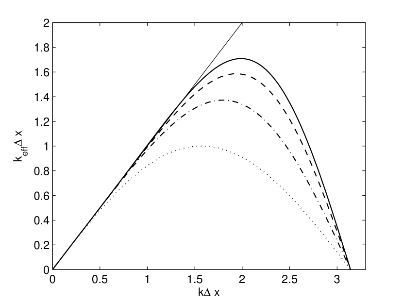
Figure 2: Effective wave number $k_{eff}\Delta x$ versus $k\Delta x$ for different numerical schemes. Dotted, dash-dotted, dashed, and solid curves represent classic 2nd, 4th, 6th, and DRP 4th order schemes correspondingly.

The plots of numerical wave number $k_{eff}\Delta x$ versus $k\Delta x$ for different numerical schemes are shown in Figure 2. Dotted, dash-dotted, dashed, and solid curves represent classic 2nd, 4th, 6th, and DRP 4th order schemes correspondingly. One can see that the 4th-order DRP scheme describes short waves more accurately than the classic 6th-order scheme.

Waves with wavelength less than $4\Delta x$ are not resolved by the numerical scheme (9). They lead to point-to-point oscillations of the solution that can cause a numerical instability. Such waves have to be filtered out. We used the following digital filter of the 6th-order to eliminate unresolved short wave component from the solution:

$$f_{sm}(x)=f(x)-\sigma_{f}D(x)=f(x)-\sigma_{f}\sum_{m=-3}^{3}d_{m}f(x+m\Delta x),$$ (15)

where $f$ is the original grid function, $f_{sm}$ is the filtered grid function, $D(x)$ is the damping function, $\sigma_{f}$ is the constant between 0 and 1, determining the filter strength. The frequency response function $G(k)$ of the filter relates the Fourier images of the original $\tilde{f}$ and filtered $\tilde{f}_{sm}$ grid functions as follows $\tilde{f}_{sm}(k)=G(k)\tilde{f}(k)$. In this paper, the coefficients $d_{m}$ of the digital filter have been chosen in such a way that

$$G(k\Delta x)=1-\sum_{m=-3}^{3}d_{m}e^{imk\Delta x}=1-\sin^{6}\left(\frac{k\Delta x}{2}\right).$$ (16)

Coefficients $d_{m}$ of the digital filter are symmetric:

$$\begin{array}[]{l}\displaystyle d_{0}=\frac{5}{16},\quad d_{1}=d_{-1}=-\frac{15}{64},\quad d_{2}=d_{-2}=\frac{3}{32},\quad d_{3}=d_{-3}=-\frac{1}{64}.\end{array}$$ (17)

Using the technique proposed by Carpenter et al. (1993) we have found a stable 3rd-order boundary closure of the explicit dispersion-relation-preserving inner scheme (9) with coefficients given by (14). Obtained boundary closure has summation-by-parts properties. This approach is based on the implicit Padé approximation of spatial derivatives near the boundaries

$$\mbox{\boldmath$P$}\frac{\partial\mbox{\boldmath$q$}}{\partial x}=\mbox{\boldmath$Qq$},$$ (18)

where matrices $P$ and $Q$ satisfy the following conditions:

1. $P$ is symmetric non-singular matrix ($\mbox{\boldmath$P$}=\mbox{\boldmath$P$}^{T}$),

2. $P$ is positive-definite matrix ($\mbox{\boldmath$U$}^{T}\mbox{\boldmath$PU$}>0$ for $\forall\;\mbox{\boldmath$U$}$),

3. $Q$ is almost skew-symmetric matrix, except corner top left and bottom right elements ($\mbox{\boldmath$Q$}+\mbox{\boldmath$Q$}^{T}=|q_{0,0}|\mbox{diag}(-1,0,\ldots,1)$)

4. $q_{N,N}>0,\quad q_{0,0}=-q_{N,N}$.

Taking into account these properties, one can write explicitly the top left corners of matrices $P$ and $Q$:

$$\begin{array}[]{l}\mbox{\boldmath$Q$}=\left(\begin{array}[]{ccccccccc}q_{00}&q_{01}&q_{02}&q_{03}&0&0&0&0&\\ -q_{01}&0&q_{12}&q_{13}&a_{3}&0&0&0&\\ -q_{02}&-q_{12}&0&q_{23}&a_{2}&a_{3}&0&0&\cdots\\ -q_{03}&-q_{13}&-q_{23}&0&a_{1}&a_{2}&a_{3}&0&\\ 0&-a_{3}&-a_{2}&-a_{1}&0&a_{1}&a_{2}&a_{3}&\\ &&&\vdots&&&&&\ddots\\ \end{array}\right),\\ \mbox{\boldmath$P$}=\left(\begin{array}[]{cccccc}p_{00}&p_{01}&p_{02}&p_{03}&0&\\ p_{01}&p_{11}&p_{12}&p_{13}&0&\\ p_{02}&p_{12}&p_{22}&p_{23}&0&\cdots\\ p_{03}&p_{13}&p_{23}&p_{33}&0&\\ 0&0&0&0&1&\\ &&\vdots&&&\ddots\end{array}\right),\end{array}$$ (19)

where coefficients $a_{i}$ of the inner scheme are defined in (14). Expanding the left and right-hand sides of (18) in Taylor series at the top boundary and equating terms of the same order of $\Delta x$, one can obtain a system of linear equations for coefficients $p_{ij}$ and $q_{ij}$. Not all of these equations are independent, so the solution depends on two free parameters $p_{33}$ and $p_{23}$:

$$\begin{array}[]{l}\displaystyle p_{00}=-\frac{83}{108}+p_{33},\quad p_{11}=-8p_{23}-15p_{33}-\frac{34016-14973\pi}{54(15\pi-32)},\vspace{5pt}\\ \displaystyle p_{22}=\frac{1727}{108}-8p_{23}-15p_{33},\quad p_{01}=p_{23}-\frac{8(6\pi-29)}{27(15\pi-32)},\vspace{5pt}\\ \displaystyle p_{02}=3p_{33}-\frac{10929\pi-24352}{216(15\pi-32)},\quad p_{03}=-p_{23}-4p_{33}-\frac{58528-26949\pi}{432(15\pi-32)},\vspace{5pt}\\ \displaystyle p_{12}=7p_{23}+12p_{33}-\frac{84813\pi-188192}{432(15\pi-32)},\quad p_{13}=3p_{33}-\frac{8691\pi-17504}{216(15\pi-32)},\vspace{5pt}\\ \displaystyle q_{00}=-\frac{1}{2},\quad q_{01}=-2p_{23}-6p_{33}-\frac{212960-95451\pi}{864(15\pi-32)},\vspace{5pt}\\ \displaystyle q_{02}=4p_{23}+12p_{33}-\frac{42537\pi-93856}{216(15\pi-32)},\quad q_{03}=-2p_{23}-6p_{33}-\frac{176288-81177\pi}{864(15\pi-32)},\vspace{5pt}\\ \displaystyle q_{12}=-6p_{23}-18p_{33}-\frac{180896-83661\pi}{288(15\pi-32)},\quad q_{13}=4p_{23}+12p_{33}-\frac{38451\pi-80992}{216(15\pi-32)},\vspace{5pt}\\ \displaystyle q_{23}=-2p_{23}-6p_{33}-\frac{152288-76731\pi}{864(15\pi-32)}.\end{array}$$ (20)

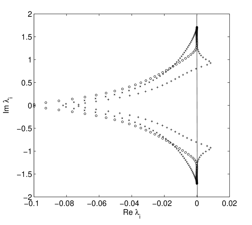
Figure 3: Eigenvalues of the DRP spatial discretization operator for scalar advection equation on complex plane for different choices of the coefficient $p_{23}$. Symbols plus correspond to the scheme $p_{23}=1/30,\>p_{33}=31/32$ which does not exhibit an asymptotic stability. Circles and crosses represent choices of $p_{23}=1/80,\,-1/10$ and $p_{33}=125/128,\>65/64$ correspondingly. Both schemes are asymptotically stable.

To satisfy a condition of positive definiteness it is sufficient to choose matrix elements $p_{33}$ and $p_{23}$ in such a way, that the signs of coefficients of a characteristic polynomial alternate. However, this property does not guarantee a boundedness of the solution for all times, which is called asymptotic stability. To make a solution be bounded for all times, all eigenvalues of the spatial discretization operator $L_{ikj}$ from Eq.(7), incorporated with the boundary conditions, must have non-positive real parts. Details of this procedure can be found in (Carpenter et al., 1993). Due to complexity of the original 3D problem, we have tested a stability of the scheme on 1D advection problem. Distribution of eigenvalues of the DRP spatial discretization operator in the complex plane for different choices of the pairs of coefficients ($p_{23}$, $p_{33}$) is shown in Fig. 3. Symbols plus correspond to the scheme $p_{23}=1/30,\>p_{33}=31/32$, which does not exhibit asymptotic stability. Circles and crosses represent choices (1/80, 125/128) and (-1/10, 65/64) of coefficients $(p_{23},p_{33})$ correspondingly. Both schemes are asymptotically stable.

Acoustic sources have been added to the right-hand side of equations (1). We used sources of two types. If we add a scalar function $\Phi(x,y,z,t)$ to the right-hand side of z-component of momentum equation, this term can be combined with the gravity term and interpreted as a source of z-component of force. If we add a gradient of a scalar function $\nabla\Phi(x,y,z,t)$ to the right-hand side of all momentum equations, these terms can be combined with components of the pressure gradient and interpreted as a pressure source. Acoustic sources are spatially localized and have finite lifetime. Spatial dependence is given by Gaussian spherically symmetric function with semi-width of 2-3 grid nodes. We experimented with two different time dependencies of acoustic sources: one period of sin function $\sin[\omega(t-t_{0})],\;t_{0}\leq t\leq t_{0}+2\pi/\omega$ and Ricker’s wavelet $(1-2x^{2})e^{-x^{2}},\;x=[\omega(t-t_{0})/2-\pi],\;t_{0}\leq~{}t\leq~{}t_{0}+4\pi/\omega$. Such time dependencies were chosen because such sources are not monochromatic and have spectral power localized around central frequency $\omega/2\pi$, but spectral power is not too spread out. Single or multiple acoustic sources can be added to the right hand side of equations. Multiple sources are randomly distributed at some depth (in our case it was 350 km) and initiated independently at arbitrary moments of time. Amplitudes and frequencies are randomly distributed on intervals [0, 1] and [2 mHz, 8 mHz] correspondingly. Thickness of both (top and bottom) PMLs equals 5 grid nodes.

Calculation of the acoustic spectrum requires long term simulations, so besides the asymptotic stability we have to prevent a spurious reflection of acoustic waves from the boundaries back to the computational domain. In this paper we follow Hu (1996), who proposed a procedure to construct the PML for the Euler equations. It can be proofed that for a homogeneous medium and uniform mean flow without gravity PML absorbs waves without reflection for any angle of incidence and frequency. We set non-reflecting boundary conditions based on the PML at the top and bottom boundaries of the domain. The lateral boundary conditions are periodic. Inside the PML independent variables $q$ are split into sub-components $\mbox{\boldmath$q$}_{1},\mbox{\boldmath$q$}_{2},\mbox{\boldmath$q$}_{3}$ such that $\mbox{\boldmath$q$}=\mbox{\boldmath$q$}_{1}+\mbox{\boldmath$q$}_{2}+\mbox{\boldmath$q$}_{3}$. Thus, in the PML 3D system (1) is split into 1D+1D+1D system of coupled locally one dimensional equations

$$\begin{array}[]{l}\displaystyle\frac{\partial\mbox{\boldmath$q$}_{1}}{\partial t}+\frac{\partial\mbox{\boldmath$F$}(\mbox{\boldmath$q$})}{\partial x}=0,\\[7.0pt] \displaystyle\frac{\partial\mbox{\boldmath$q$}_{2}}{\partial t}+\frac{\partial\mbox{\boldmath$G$}(\mbox{\boldmath$q$})}{\partial y}=0,\\[7.0pt] \displaystyle\frac{\partial\mbox{\boldmath$q$}_{3}}{\partial t}+\frac{\partial\mbox{\boldmath$H$}(\mbox{\boldmath$q$})}{\partial z}=\mbox{\boldmath$S$}(\mbox{\boldmath$q$},t)-\sigma_{z}\mbox{\boldmath$q$}_{3},\end{array}$$ (21)

where $\Delta t\,\sigma_{z}=0.05+\sigma_{max}(Z/D)^{2}$ is the damping factor, $Z$ is the vertical coordinate inside the PML counted off from the interface of the PML with the inner region, D is the depth of the PML. Values of $\sigma_{max}$ at the top and bottom boundaries are 0.3 and 1.0 correspondingly. In the paper of F.Q. Hu a quadratic dependence of $\sigma$ on the coordinate $Z$ is used. We were forced to add a small constant term to stabilize the PML in the presence of gravity. It is important to note, that vectors $F$, $G$, and $H$ depend only on unsplit variable $q$. Although $\mbox{\boldmath$q$}_{1}$, $\mbox{\boldmath$q$}_{2}$, and $\mbox{\boldmath$q$}_{3}$ are not defined outside the PML, the variable $q$, which is used for calculation of the spatial derivatives, is defined everywhere in the computational domain. Hence, inside the PML near the interface with the inner region we can use the same centered stencil as for the inner points. Near the top and bottom boundaries the implicit Pade approximation (18) is used which guarantees numerical stability of the scheme. We smoothly joined the chromospheric model provided by Vernazza et al. (1976) with the top of the standard solar model by Christensen Dalsgaard and established the top non-reflecting boundary condition based on the PML in the chromosphere above the temperature minimum. This simulates a realistic situation when not all waves are reflected by the photosphere. Waves with frequencies higher than the acoustic cut-off frequency pass through the photosphere and will be absorbed by the PML layer.

3 Numerical examples

For validation of the code we chose 1D initial boundary value problem (IBVP) for linearized Euler equations with constant gravity $g_{0}=const$:

$$\begin{array}[]{l}\displaystyle\frac{\partial\rho^{\prime}}{\partial t}+\frac{\partial}{\partial x}(\rho_{0}u^{\prime})=0,\\[9.0pt] \displaystyle\frac{\partial}{\partial t}(\rho_{0}u^{\prime})+\frac{\partial p^{\prime}}{\partial x}=g_{0}\rho^{\prime},\\[9.0pt] \displaystyle\frac{\partial}{\partial t}(\rho_{0}\xi)=\rho_{0}u^{\prime},\\[9.0pt] \displaystyle p^{\prime}=a_{0}^{2}\rho^{\prime}+(\gamma-1)g_{0}(\rho_{0}\xi),\end{array}\begin{array}[]{l}0\leq x\leq 1,\quad t\geq 0,\\[9.0pt] \rho^{\prime}(0,t)=\rho^{\prime}(1,t)=0,\\[9.0pt] \rho^{\prime}(x,0)=f(x),\quad\rho_{0}(x)u^{\prime}(x,0)=0,\\[9.0pt] \displaystyle\rho_{0}(x)\xi(x,0)=-\int\limits_{0}^{x}f(\eta)\;\mbox{d}\eta,\end{array}$$ (22)

where $\xi$ is the displacement. We need to know $\xi$ to calculate the Eulerian perturbation of pressure $p^{\prime}$. Actually, the combination $\rho_{0}\xi$ is used as a variable, so we group them together in equations. Initial conditions for $\xi$ must be consistent with the initial conditions for $\rho^{\prime}$. They are related by the continuity equation. Waves are adiabatic, the background model $p_{0},\rho_{0}$ is hydrostatic and isothermal $p_{0}/\rho_{0}=const$. The last equation in the system (22) is the adiabatic relation (2) written for the isothermal background model. Variable $x$ represents here the depth from the surface. The system (22) is written in the same conservative form as the original system (1). This problem was chosen for testing the code because it shows all characteristic behavior of the realistic solution and yet not too complicated and can be solved analytically. Formally, the variable $\rho_{0}\xi$ can be eliminated using the continuity equation in 1D, and system (22) can be reduced to the system of two equations. However, in 3D $\rho_{0}\xi$ cannot be eliminated. To have the test example as close to the real case as possible, we left this variable and solved numerically the full system (22). Analytical solution of these equations can be obtained by the method of separation of variables

$$\begin{array}[]{l}\displaystyle\rho^{\prime}(x,t)=e^{x/2H}\sum_{n=1}^{\infty}A_{n}\sin\pi nx\cos\lambda_{n}a_{0}t,\\[9.0pt] \displaystyle\xi(x,t)=e^{-x/2H}\sum_{n=1}^{\infty}B_{n}(\sin\pi nx-2\pi nH\cos\pi nx)\cos\lambda_{n}a_{0}t,\\[9.0pt] \displaystyle A_{n}=2\int_{0}^{1}f(\eta)e^{-\eta/2H}\sin\pi n\eta\mbox{d}\eta,\quad B_{n}=-\frac{2HA_{n}}{1+4\pi^{2}n^{2}H^{2}},\\[9.0pt] \displaystyle\lambda_{n}=\sqrt{\frac{1}{4H^{2}}+\pi^{2}n^{2}},\quad H^{-1}=\frac{\gamma g_{0}}{a_{0}^{2}}.\end{array}$$ (23)

The following distribution of density perturbation $f(x)$ was chosen as the initial condition for $\rho^{\prime}$:

$$f(x)=\left\{\begin{array}[]{l}10^{4}[(x-0.5)^{2}-0.001]^{2}\quad\mbox{if}\;\;0.4\leq x\leq 0.6\\ 0\end{array}\right.$$ (24)

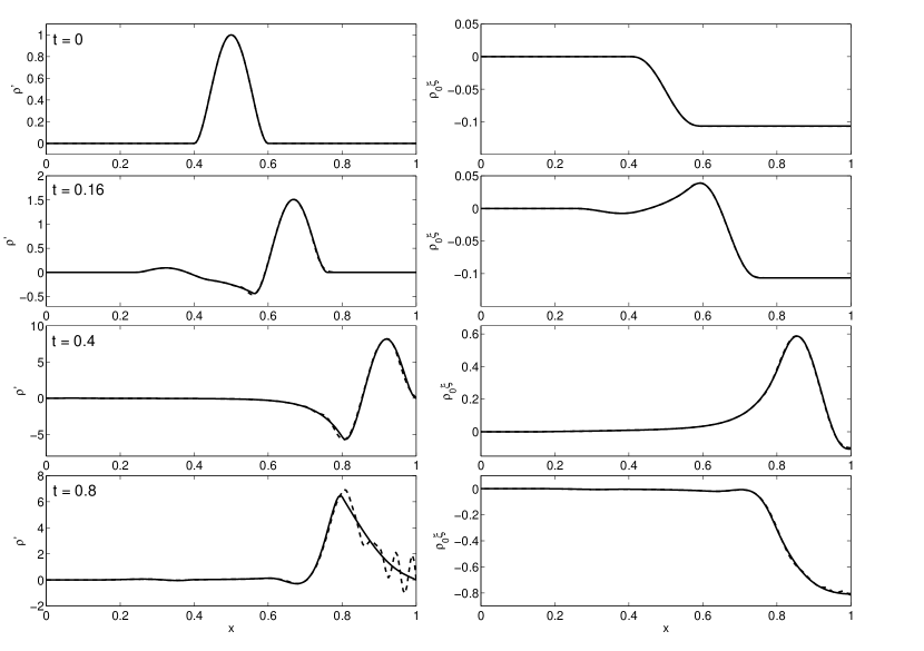
Figure 4: Solution of the IBVP (22) for the isothermal hydrostatic background model. Density and displacement are shown on the left and right panes correspondingly. Solid curve represents the exact solution, dashed one shows the classic 2/1 numerical solution. The high order DRP 4/3 numerical solution is indistinguishable from the exact one. After hitting the boundary classic 2/1 solution changes the global order of accuracy to 1, because boundary conditions are realized only with the 1st order of accuracy.

Solution of the initial boundary value problem (22) for different moments of time with the initial density distribution given by (24) and parameters $a_{0}=1$, $\gamma=5/3$, $g_{0}=10$, $\Delta t=2\cdot 10^{-3}$, $N=200$ (number of grid nodes) is shown in Figure 4. The left column represents the density perturbation, the right one shows the vertical displacement. The solid curve is the exact solution (23). The dashed curve represents the low-order (classic 2/1) numerical solution which uses the 2nd-order classic central difference approximation of spatial derivatives for inner points with the one sided 1st-order scheme at the boundaries. The high-order numerical solution is indistinguishable from the exact one. It uses the DRP 4/3 scheme (dispersion-relation-preserving spatial discretization of the 4th order for inner points with the stable boundary closure of the 3rd order consistent with the inner scheme). The bottom panels give the profiles of density and displacement after reflection from the bottom boundary. One can see, that the second order solution approximates the exact one well enough before the wave hits the boundary. After this the accuracy of the solution switches from the second to the first order. Solution becomes too dispersive which causes nonphysical oscillations. The high-order solution based on DRP 4/3 scheme reproduces the exact solution well even after $30000\div 40000$ iterations and 20$\div$30 reflections from boundaries. This test shows that the high-order DRP numerical scheme does not introduce a noticeable damping or dispersion even on big intervals of integration. These simulations also test an accuracy and stability of the numerical boundary conditions.

To test the efficiency of the PML for non-uniform isothermal background model we compared the numerical solution of (22) with the PML established at the top boundary with the exact solution of the same problem for infinite interval $-\infty\leq x\leq\infty$:

$$\rho^{\prime}(x,t) = \frac{1}{2}f(x+a_{0}t)e^{-a_{0}t/2H}+\frac{1}{2}f(x-a_{0}t)e^{a_{0}t/2H}-$$ (25)

$$\frac{a_{0}t}{4H}\;e^{x/2H}\int\limits_{x-a_{0}t}^{x+a_{0}t}e^{-\eta/2H}\frac{J_{1}(\sqrt{a_{0}^{2}t^{2}-(x-\eta)^{2}}/2H)}{\sqrt{a_{0}^{2}t^{2}-(x-\eta)^{2}}}f(\eta)\;\mbox{d}\eta.$$

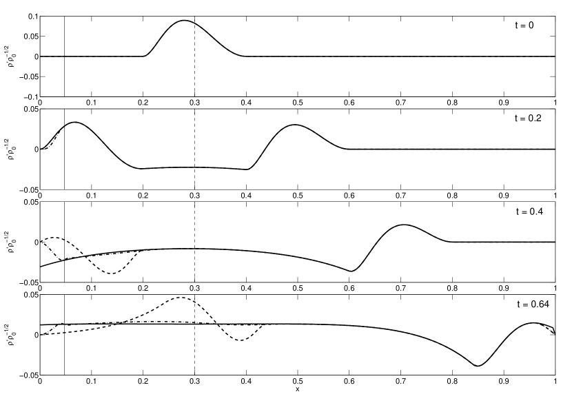
Figure 5: Density perturbation with removed exponential factor $\rho^{\prime}/\sqrt{\rho_{0}}$ is plotted. The solid line represents the exact solution for infinite interval (25), the dash-dotted line represents the numerical solution with the PML at the top boundary, and the the dashed line represents the exact solution (23) for reflecting left boundary. The vertical solid and dashed lines mark positions of the PML interface and initial perturbation correspondingly.

Bottom boundary condition for the numerical solution remains reflecting, because the bottom PML is inconsistent with the initial conditions for $\xi(x,t)$. At the bottom boundary in the initial moment of time $\xi(1,0)<0$ (see the top right panel of Figure 4). If we established PML at the bottom, it would damp $\xi$ to zero value, generating non-physical perturbations near the bottom boundary which corrupt the solution. The analytical solution (25) does not contain reflected waves, because all initial perturbations propagate to infinity. This solution can be used as a reference solution for determining the damping properties of the top PML. Results are shown in Figure 5 at the moments of time $t=$ 0, 0.2, 0.4, and 0.64. The value $\rho^{\prime}/\sqrt{\rho_{0}}$ (density perturbation with removed exponential factor) is plotted. The solid line represents the exact solution (25), the dash-dotted line represents the numerical solution with PML at the top boundary, and the the dashed line represents the exact solution (23) for the reflecting top boundary. The solid vertical line marks position of the interface between the top PML and inner region. The dashed vertical line shows position of the initial perturbation. The top PML reduces the amplitude of reflected wave by factor 20$\div$40.

Our original 3D system contains acoustic sources explicitly depending on time in the right hand side of the momentum equations. We have tested the code in presence of sources on the same problem (22) with the pressure source term

$$\begin{array}[]{l}\displaystyle\frac{\partial\rho^{\prime}}{\partial t}+\frac{\partial}{\partial x}(\rho_{0}u^{\prime})=0,\\[9.0pt] \displaystyle\frac{\partial}{\partial t}(\rho_{0}u^{\prime})+\frac{\partial p^{\prime}}{\partial x}=g_{0}\rho^{\prime}-\frac{\partial\Phi(x,t)}{\partial x},\\[9.0pt] \displaystyle\frac{\partial}{\partial t}(\rho_{0}\xi)=\rho_{0}u^{\prime},\\[9.0pt] \displaystyle p^{\prime}=a_{0}^{2}\rho^{\prime}+(\gamma-1)g_{0}(\rho_{0}\xi),\end{array}\begin{array}[]{l}0\leq x\leq 1,\quad t\geq 0,\\[9.0pt] \rho^{\prime}(0,t)=\rho^{\prime}(1,t)=0,\\[9.0pt] \rho^{\prime}(x,0)=0,\quad\rho_{0}(x)u^{\prime}(x,0)=0,\\[9.0pt] \displaystyle\rho_{0}(x)\xi(x,0)=0.\end{array}$$ (26)

For test purposes we chose gaussian shaped harmonic source function as follows

$$\Phi(x,t)=e^{-\textstyle\left(\frac{x-h_{src}}{\sigma}\right)^{2}}\sin(\omega_{0}t),$$ (27)

The system (26) can be solved analytically by quadratures

$$\begin{array}[]{l}\displaystyle\rho^{\prime}(x,t)=\int\limits_{0}^{t}\!\!\int\limits_{0}^{1}\frac{\partial^{2}\Phi(\eta,\tau)}{\partial\eta^{2}}G(x,\eta,t-\tau)\;\mbox{d}\eta\mbox{d}\tau,\\[15.0pt] \displaystyle G(x,\eta,\tau)=2\;e^{(x-\eta)/2H}\sum_{n=1}^{\infty}\frac{\sin\lambda_{n}a_{0}\tau}{\lambda_{n}a_{0}}\sin\pi nx\sin\pi n\eta,\\[15.0pt] \displaystyle\lambda_{n}=\sqrt{\frac{1}{4H^{2}}+\pi^{2}n^{2}}.\end{array}$$ (28)

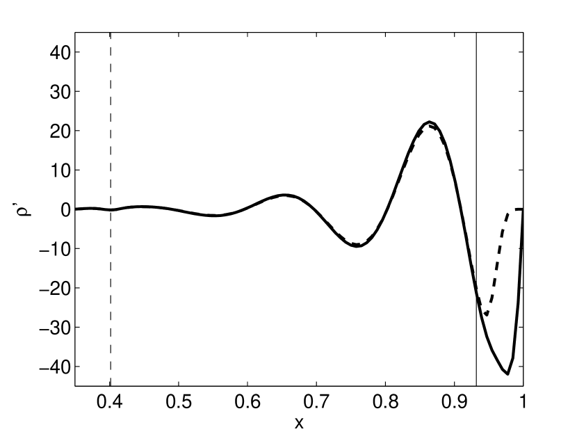
Figure 6: Solution of the IBVP (26) for the isothermal hydrostatic background model in presence of the source. The solid curve represents the exact solution with zero boundary conditions for $\rho^{\prime}$. The dashed line represents DRP 4/3 numerical solution of (26) with non-reflecting top and bottom boundaries. Numerical solution is damped effectively by the absorbing layer.

The results of numerical simulations with the source function given by (27) and parameters $N=120$, $\Delta t=2\cdot 10^{-3}$, $a_{0}=1$, $\gamma=5/3$, $g_{0}=10$, $h_{src}=0.4$, $\omega_{0}=10\pi$, $\sigma=0.0178$ are shown in Figure 6. The non-reflecting boundary conditions are established on the top and bottom boundaries for numerical solution. The solid curve represents the exact solution of (6) with zero boundary conditions for $\rho^{\prime}$ established at $x=0$ and $x=1$. The dashed line represents DRP 4/3 numerical solution of (6) with non-reflecting top and bottom boundaries. The vertical dashed line marks the position of the source. The vertical solid line shows the position of the interface between the inner region of the computational domain and the non-reflecting PML. The numerical solution reproduces the exact one well in the inner region, and is effectively damped by the absorbing layer, preventing unwanted reflection from the bottom boundary.

Numerical simulations of propagation of waves in 3D from a single source inside the Sun are shown in Figure 7. The Brunt-Väisälä frequency of the standard solar model with smoothly joined chromosphere was modified near the surface to make the model stable against convection. Such modified model was chosen as the background model. Non-reflecting boundary conditions (PMLs) were established at the top and bottom boundaries. The top layer was established at the height of 500 km above the photosphere in the region of the temperature minimum. This layer absorbs all waves with frequencies higher than the acoustic cut-off frequency which pass to the chromosphere and do not affect reflection of waves with lower frequencies, because these waves are reflected from layers below the photosphere. Lateral boundary conditions are periodic. The computational domain of size 120$\times$120$\times$50 Mm³ was covered by the uniform grid of size 720$\times$720$\times$300 nodes with spatial intervals $\Delta x=\Delta y=\Delta z=170$ km. The time step $\Delta t=1$ sec was chosen from stability condition. The Gaussian spherically symmetric pulse source of z-component of force

$$\Phi(x,t)=\exp\left[-\left(\frac{\mbox{\boldmath$r-r$}_{src}}{\sigma}\right)^{2}\right]\sin(\omega_{0}t),\quad 0\leq t\leq 2\pi/\omega_{0}.$$ (29)

with $\sigma=0.4$ Mm was placed at the depth of 3.4 Mm below the photosphere. For such a choice of $\sigma$ semi-width of the source equals approximately 4 grid nodes. The time dependent part is just one period of sin-function with $\omega_{0}=2.5$ mHz. Figure 7 shows snapshots of the density perturbation from such a source at $t=11.7$ min (left column) and $t=21.7$ min (right column). The top row represents the vertical slices of the computational domain, the bottom row shows the horizontal slices at a height of 350 km above the photosphere. The thin horizontal line at $z=0$ represents the photosphere. The left column shows the disturbance from the direct wave, generated by the source. The right column shows the wave reflected from the photosphere. The reflected wave front is broader and has less amplitude, because our source has finite lifetime (one period of sine) and generates high frequency waves which pass through the photosphere. Such waves are absorbed by the top non-reflecting layer and do not make a contribution to the amplitude of the reflected wave.

4 Results and Discussion

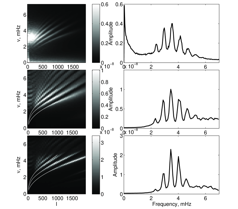
Figure 9: Acoustic spectra obtained from observations and simulations with different heights of the top boundary (the left panes). Starting from the top: observations, simulations with $h_{top}$=500 km, simulations with $h_{top}$=1750 km. The thin white curves on the left panes show position of observational ridges for $f$, $p_{1}$, and $p_{2}$ modes. The right panes show cuts of k-$\omega$ diagrams from left panes at l=584. For simulations with high top boundary without additional damping (bottom row) acoustic modes trapped in the domain distort the shape of the acoustic spectrum.

The developed numerical method and code have been used for simulation of the acoustic wave field generated by multiple acoustic sources inside the Sun. We found that the height of the PML affects absorbing properties of the top boundary and the shape of the acoustic spectrum (k-$\omega$ diagram). Reflection from the top boundary is a wave process. The waves are reflected not from the fixed level but from some vertical region. Region with the acoustic cut-off frequency greater than the wave frequency $\omega_{c}>\omega$ acts as a potential barrier for such waves. Even if the wave frequency is less than the acoustic cut-off frequency waves penetrate to this region with exponentially decaying amplitude. If the thickness of the barrier is finite waves can leak through it. This process is similar to the tunneling effect in quantum mechanics. This happens in the real Sun as well. We studied behavior of the solution for different heights of the top boundary. All depths and heights are calculated from the level of the photosphere ($r=R_{sun}$ in the Christensen-Dalsgaard’s standard solar model S). The background model varies fast in the region above the temperature minimum. To be able to simulate propagation of acoustic waves in the chromosphere we were forced to reduce the vertical spatial step to $\Delta z=50$ km to preserve the numerical stability. To keep the horizontal size of the domain as in previous simulations without significant increasing number of grid nodes the horizontal spatial steps were chosen 3 times bigger $\Delta x=\Delta y=3\Delta z=150$ km. To satisfy the Courant stability condition for the explicit scheme, the time step was reduced to $\Delta t=0.68$ sec. The computational domain of size 122.2 Mm $\times$ 122.2 Mm $\times$ 32 Mm is covered by the uniform grid of size 816$\times$816$\times$640. Sources of z-component of force with random frequencies were randomly distributed at the depth of 350 km. Sources are initiated at random moments of time (one source per time step) and depend on time as Ricker’s wavelet with central frequency from range 2$\div$8 mHz. In the Sun we have some damping due to the turbulent viscosity. We simulated this additional viscosity by adding a damping term $-\sigma_{d}q_{z}$ to the right hand side of z-momentum equation in the region above the photosphere and smoothly fading to zero below. The time dependence of RMS (root mean square) wave amplitude averaged along the horizontal plane at the height of 300 km above the photosphere for different heights $h_{top}$ of the top boundary and different values of the damping coefficient $\sigma_{d}$ is shown in Figure 8. The RMS amplitude for the high PML established at the height of $h_{top}=1750$ km without additional damping $\sigma_{d}$ = 0 is shown by the solid curve I. The RMS amplitudes for the same height of the top PML and $\sigma_{d}$ = 0.3, 0.6, and 1.0 are plotted by solid lines II, III, and V correspondingly. In the last case the RMS amplitude reaches an equilibrium state. The curve IV corresponds to the low PML, established at the height of 500 km above the photosphere without additional damping in the inner region $\sigma_{d}$ = 0. RMS amplitude reaches an equilibrium state in this case as well, because the acoustic modes leak through the acoustic potential barrier and their exponential tails reach the top absorbing boundary, which adds an additional damping and stabilizes the amplitude. The top boundary with the height of 1750 km is set high enough and does not affect modes with frequencies less than the acoustic cut-off frequency. Energy is continuously pumped to the system by acoustic sources. The bottom boundary is deep enough that some modes resolved by numerical scheme have turning points above the bottom boundary. Such modes are trapped in the domain, the total energy increases, and the RMS amplitude does not reach an equilibrium state. This distorts the acoustic power spectrum and changes the amplitude ratio of trapped modes and modes that can be absorbed at the top and/or bottom boundaries. The left panes in Figure 9 show the acoustic power spectra obtained from observations (top), simulations without damping with low (500 km) top boundary (middle), and high (1750 km) top boundary (bottom). The right panes show the vertical cuts of corresponding k-$\omega$ diagrams at $l=584$. The bottom left pane (high top boundary) shows presence of g- modes in simulations. They appear because our background model is convectively stable in the thin layer below the photosphere. In the real Sun, this layer is convectively unstable, and thus the g- modes do not propagate. Energy leakage through the acoustic potential barrier in the case of low top boundary (middle row) damps all modes uniformly and does not change the shape of the acoustic spectrum. So the height of the top boundary can be used for controlling the damping rate without distortion of the acoustic spectrum.

5 Conclusion

Developed linear 3D code for propagation of acoustic waves inside the Sun uses the realistic equation of state and realistic non-reflecting boundary conditions which permits to simulate accurately reflection of waves from the top boundary. Waves with frequencies less then the acoustic cut-off frequency are reflected from the photosphere, and waves with higher frequencies pass to the chromosphere. The top non-reflecting boundary absorbs such waves. Establishing the top boundary high enough in the chromosphere leads to the trapping of some modes in the domain and increasing their amplitudes with time, which distorts the shape of the acoustic spectrum. Energy leakage through the acoustic potential barrier in case of the low (500 km) top boundary leads to an additional uniform damping of all modes which stabilizes the amplitude and does not distort the spectrum. The height of the non-reflecting top boundary can be used as a parameter for controlling of the damping rate in the system. The acoustic spectrum obtained from simulated wave field shows existence of p-, and f-modes. The simulated acoustic spectrum is good agreement with observations.

This code has been used by (Parchevsky & Kosovichev, 2006) to model the effects of non-uniform spatial distribution of acoustic sources in sunspot regions. Their results showed that this effect can explain at least a half of the observed amplitude reduction in sunspots. The code can be used for studying details of interaction of waves with inhomogeneities of solar structure and for producing artificial data for testing an accuracy of helioseismic inversion as well, as for studying of propagation of acoustic waves in the chromosphere and reflecting properties of the photosphere. Future simulations will include subsurface flows and magnetic field.

6 Acknowledgements

This research is supported by the Living With the Star NASA grant NNG05GM85G. The calculations were performed on Columbia supercomputer at NASA Ames Research Center (NASA Advanced Supercomputing Division).

Figure 7: Snapshots of the density perturbation from spherically symmetric Gaussian pulse of a z-component of force at $t=11.7$ min (left column) and $t=21.7$ min (right column). The top row represents the vertical slices of the computational domain, the bottom row shows the horizontal slices at a height of 350 km above the photosphere. Thin horizontal line at $z=0$ represents the photosphere. The depth of the source equals 3.5 Mm below the photosphere.

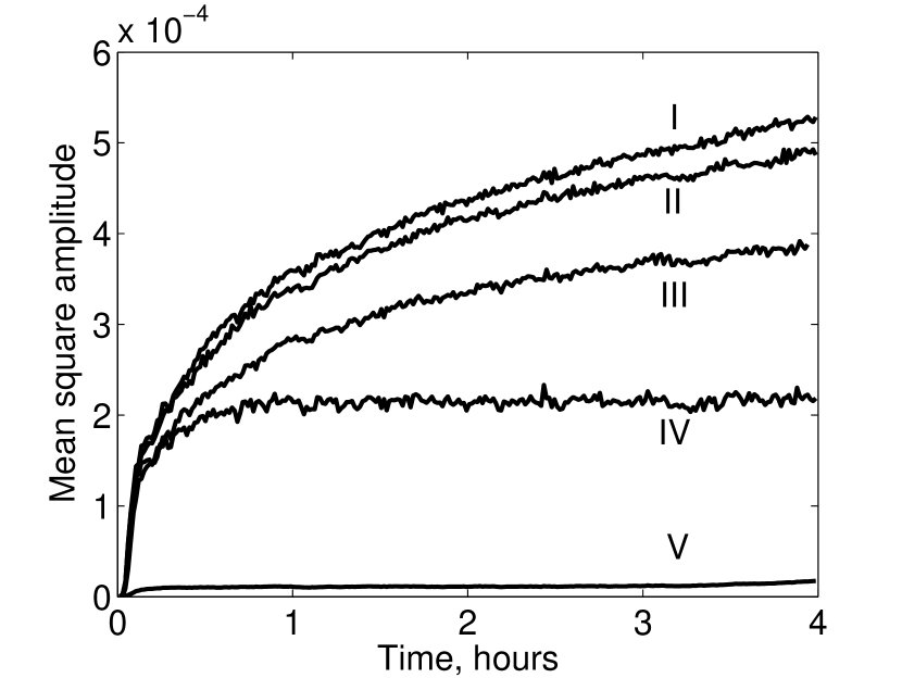
Figure 8: Wave amplitude averaged along the horizontal plane at the height of 300 km above the photosphere for different heights of the top boundary and different damping coefficients. The curve I corresponds to the high top boundary, established at 1750 km above the photosphere without any additional damping. The curves II, III, V correspond to the same boundary conditions, but different values of damping coefficient $\sigma_{d}$ = 0.3, 0.6, 1.0. The curve IV corresponds to the low top boundary, established at 500 km without artificial damping.

References

- Birch et al. (2001) Birch, A. C., Kosovichev, A. G., Price, G. H., & Schlottmann, R. B. 2001, ApJ, 561, L229
- Birch & Felder (2004) Birch, A. C., & Felder, G. 2004, ApJ, 616, 1261
- Carpenter et al. (1993) Carpenter, M.H., Gottlieb, D., & Abarbanel, S. 1993, J. Comput. Phys. 108, 272.
- Christensen-Dalsgaard et al. (1996) Christensen-Dalsgaard, J., et al. 1996, Science, 272, 1286.
- Couvidat et al. (2004) Couvidat, S., Birch, A. C., Kosovichev, A. G., & Zhao, J. 2004, ApJ, 607, 554
- Couvidat et al. (2006) Couvidat, S., Birch, A. C., & Kosovichev, A. G. 2006, ApJ, 640, 516
- Duvall et al. (1993) Duvall, T. L., Jr., Jefferies, S. M., Harvey, J. W., & Pomerantz, M. A. 1993, Nature, 362, 430
- Georgobiani et al. (2006) Georgobiani, D., Zhao, J., Kosovichev, A., Benson, D., Stein, R. F., & Nordlund, Å. 2006, ArXiv Astrophysics e-prints, arXiv:astro-ph/0608204
- Hu (1996) Hu, F. Q. 1996, J. Comput. Phys., 129, 201.
- Rogers et al. (1996) Rogers, F. J., Swenson, F. J., & Iglesias C. A. 1996, ApJ, 456, 902.
- Jensen et al. (2001) Jensen, J. M., Duvall, T. L., Jr., Jacobsen, B. H., & Christensen-Dalsgaard, J. 2001, ApJ, 553, L193
- Kosovichev (1996) Kosovichev, A. G. 1996, ApJ, 461, L55
- Kosovichev & Duvall (1997) Kosovichev A. G., Duvall T. L. Jr. 1997, in SCORe’96: Solar Convection and Oscillations and their Relationship, eds. F. P. Pijpers, J. Christensen-Dalsgaard, & C. S. Rosenthal (Kluwer Academic Publishers, Dordrecht), 241.
- Kosovichev et al. (2000) Kosovichev A. G., Duvall T. L. Jr., & Scherrer P. 2000, Sol. Phys., 192, 159.
- Parchevsky & Kosovichev (2006) Parchevsky, K. V., & Kosovichev, A. G. 2006, ApJ, submitted
- Stein et al. (2004) Stein, R., Georgobiani, D., Trampedach, R., Ludwig, H.-G., & Nordlund, Å. 2004, Sol. Phys., 220, 229
- Shu (2002) Shu, C.-W. 2002, in Collected Lectures on the Preservation of Stability under Discretization, eds. D. Estep & S. Tavener, SIAM, 51.
- Tam & Webb (1993) Tam, C. & Webb, J. 1993, J. Comput. Phys. 107, 262.
- Thomas et al. (1982) Thomas, J. H., Cram, L. E., & Nye, A. H. 1982, Nature, 297, 485.
- Vernazza et al. (1976) Vernazza, J. E., Avrett, E. H., & Loeser, R. 1976, ApJS, 30, 1.