Oxygen pumping: mapping the reionization epoch with the CMB

Abstract

We consider the pumping of the $63.2\mu$m fine structure line of neutral OI in the high–redshift intergalactic medium (IGM), in analogy with the Wouthuysen–Field effect for the 21cm line of cosmic HI. We show that the soft UV background at $\sim 1300$Å can affect the population levels, and if a significant fraction of the IGM volume is filled with “fossil HII regions” containing neutral OI, then this can produce a non–negligible spectral distortion in the cosmic microwave background (CMB). OI from redshift $z$ is seen in emission at $(1+z)63.2\mu$m, and between $7<z<10$ produces a mean spectral distortion of the CMB with a $y$–parameter of $y=(10^{-9}-3\times 10^{-8})(Z/10^{-3}{\rm Z_{\odot}})(I_{UV})$, where $Z$ is the mean metallicity of the IGM and $I_{UV}$ is the UV background at $1300$Å  in units of $10^{-20}$ erg/s/Hz/cm²/sr. Because O is in charge exchange equilibrium with H, a measurement of this signature can trace the metallicity at the end of the dark ages, prior to the completion of cosmic reionization and is complementary to cosmological 21cm studies. While future CMB experiments, such as Planck could constrain the metallicity to the $10^{-2}Z_{\odot}$ level, specifically designed experiments could potentially achieve a detection. Fluctuations of the distortion on small angular scale may also be detectable.

1. Introduction

The first sources of light that ended the cosmic dark ages are expected to have reionized the intergalactic medium and polluted it with metals (see a review by, e.g., Loeb & Barkana 2001). To use the metal enrichment as a potential probe of the reionization epoch, recent studies have concentrated on the neutral oxygen (OI) produced by the first massive stars (Oh, 2002; Basu et al., 2004). The ionization potential of OI is only 0.2 eV higher than that of hydrogen (HI), and the two species are in charge exchange equilibrium. Therefore, oxygen is likely to be highly ionized in regions of the IGM where hydrogen is ionized. However, the recombination time for oxygen (as for hydrogen) is shorter than the Hubble time at $z\;\hbox to0.0pt{\lower 2.5pt\hbox{$\sim$}\hss}\raise 1.5pt\hbox{$>$}\;6$, indicating that oxygen can be neutral even in regions where H has been ionized but where short–lived ionizing sources have turned off, allowing the region to recombine (Oh, 2002). Indeed, Oh & Haiman (2003) show that such fossil HII regions can occupy $>50\%$ of the volume of the IGM prior to reionization. While the metal pollution of these regions is poorly understood, it is feasible that they contain significant amount of oxygen with a neutral fraction close to unity.

Previous work has proposed to exploit the scattering of UV photons by OI, and the corresponding absorption features in the spectra of quasars – the OI forest (Oh, 2002), analogous to the lower–redshift HI Lyman $\alpha$ forest (e.g., Becker et al. 2006). In the case of HI, another interesting signature from the high–redshift IGM is the 21cm hyperfine structure line, which is made detectable by UV pumping by the Lyman $\alpha$ background (the so–called Wouthuysen-Field effect; see Field 1958 or Furlanetto et al. 2006 for a recent review). Here we examine whether a similar effect occurs for OI.

Here we demonstrate that there exist OI lines with the required features: the fine structure lines of the electronic ground state, $44.1,63.2$ and $145.5\mu$m, can be pumped by $1300$ Å  photons produced by the first stars or black holes, via the Balmer $\alpha$ line of OI. We compute the spectral distortion in the CMB created by this effect, and find that it can be as high as $y\sim 10^{-7}$ if the OI metallicity at $z\sim 7$, just prior to reionization, is $\sim 10^{-2.5}{\rm Z_{\odot}}$. This distortion could be detectable with future CMB experiments, and opens the possibility of performing tomography of the reionization epoch using this effect. In combination with 21cm studies, it could yield direct measurements of the abundance and spatial distribution of metals in the high–redshift IGM.

2. Balmer-$\alpha$ pumping of OI fine structure transitions

The basic criteria for a line $0\leftrightarrow 1$ of a metal species or their ions to produce an effect analogous to the Wouthuysen–Field pumping of the HI 21cm line, are as follows: (i) abundant metals in the IGM in the required ionization state; (ii) the $0\leftrightarrow 1$ transition at a frequency suitable for detection, with Einstein coefficients small enough to allow the line to deviate from equilibrium with the CMB; (iii) the upper and lower states should be connected via allowed transitions to another state (hereafter called state 2), so that they can be “pumped” in a two–step process; (iv) a large enough background flux at the wavelength $\lambda_{02}\approx\lambda_{12}$ corresponding to the $0\leftrightarrow 2$ and $1\leftrightarrow 2$ transitions. In particular, the last criterion imposes the constraint $\lambda_{02}\;\hbox to0.0pt{\lower 2.5pt\hbox{$\sim$}\hss}\raise 1.5pt\hbox{$>$}\;1215\AA$ on the wavelength of the UV pumping photons before reionization, since neutral HI depletes the background at shorter wavelengths (Haiman et al., 2000).

We selected oxygen for our study because it can be relatively abundant at high redshifts and because the similarity of its ionization potential to that of hydrogen (we leave a systematic search through other metal lines to future work). The ground state of neutral oxygen is split into the three fine structure levels of the outermost electrons in the $n=2$ shell, hereafter denoted as $0$, $1^{a}$, and $1^{b}$. We found that among the electronic states of oxygen, these are the only one satisfying all of the criteria above and which photons would be observed in the CMB frequency band. The states $0$–$1^{a}$ and $1^{a}$–$1^{b}$ are connected by magnetic dipolar transitions [OI] ${}^{3}P_{2}\rightarrow\;^{3}P_{1}$ at 63.2 $\mu$m and ${}^{3}P_{1}\rightarrow\;^{3}P_{0}$ at 145.5 $\mu$m respectively and the states $0$–$1^{b}$ are connected by an electric quadrupolar transition ${}^{3}P_{2}\rightarrow\;^{3}P_{0}$ at 44.1 $\mu$m. We shall consider only lines involving the $0$ state ${}^{3}P_{2}$ as the lower level for the transition, since the CMB ambient field is practically unable to populate the ${}^{3}P_{1}$ state, and the 145.5 $\mu$m line will be suppressed. Since these transitions are forbidden, the spontaneous emission Einstein coefficients ($A_{44.1\mu m}=1.34\times 10^{-10}$, $A_{63.2\mu m}=8.91\times 10^{-5}$ s^-1, $A_{145.5\mu m}=1.75\times 10^{-5}$) are much smaller than the typical values for electric dipole transitions ($\sim 10^{8}{\rm s^{-1}}$), a property shared by the hydrogen 21cm line with $A_{H21}=2.85\times 10^{-15}$ s^-1.

The states $0$ and $1^{a,b}$ are connected to the excited electronic state ${}^{3}S_{1}$ in the $n=3$ shell (hereafter denoted by $2$) by means of the absorption of an OI Balmer-$\alpha$ photon with wavelength $\lambda_{20}\approx\lambda_{21}\approx 1300$Å. A schematic level diagram is shown in Figure 1. In the absence of a UV field, OI is in thermal equilibrium with the CMB and, as shown in Basu et al. (2004), resonant scattering is more important than collisionally–induced emission, except at extremely large over-densities. However, if the first stars or black holes generated a UV background at 1300Å, then the relative populations of the fine structure states 0 and 1 are modified by the two–step “pumping” transitions $0\rightarrow 2\rightarrow 1$ and $1\rightarrow 2\rightarrow 0$.

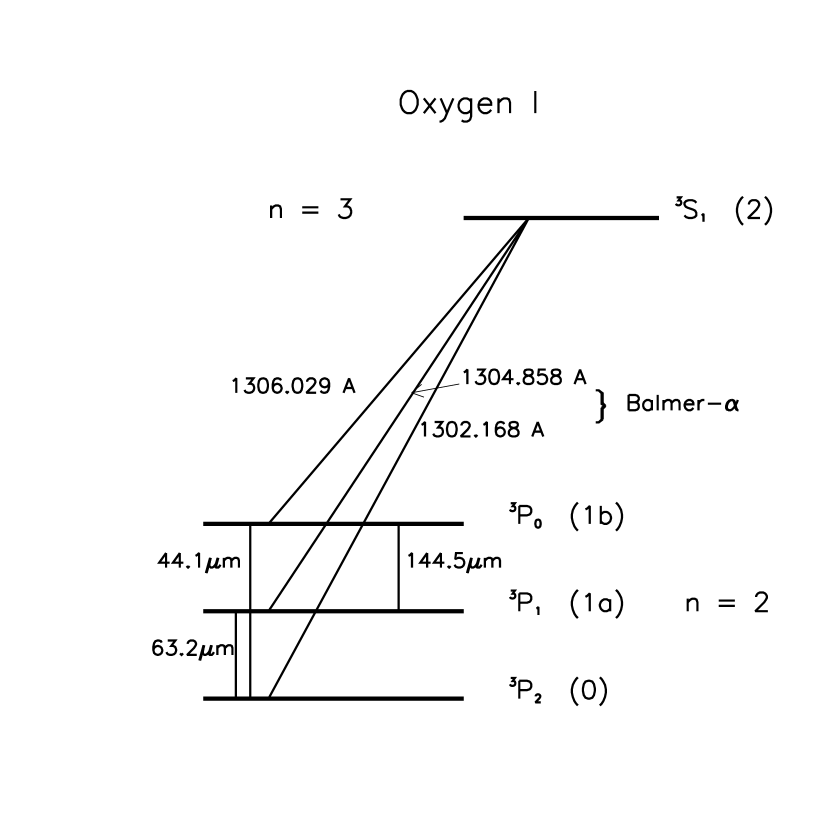
Figure 1.— Schematic representation of the transitions of neutral oxygen considered here. Note the analogy with the 21 cm transition of HI. In the 21 cm transition the relevant line corresponds to a hyperfine transition, while for OI it corresponds to a fine structure transition. The 21cm line is pumped by HI Lyman $\alpha$ photons, while the OI line is pumped OI Balmer $\alpha$ photons.

For simplicity we start by considering only one fine structure transition and only later address the combined effect. In what follows we use the indices $i,j$ to denote the two levels in the fundamental state with $i$ referring to the lowest one. For example for the 63.2.1 $\mu$m transition ($i,j$) corresponds to ($0,1^{a}$) (see fig 1). The steady state solution for the level population reads

$$\frac{n_{j}}{n_{i}}=\frac{P_{ij}^{UV}+B_{ij}I_{\nu}}{P_{ji}^{UV}+B_{ji}I_{\nu}+A_{ji}}\equiv\frac{g_{j}}{g_{i}}\exp{\left[-T_{\star,ji}/T_{S,ji}\right]}\,.$$ (1)

This equation defines the spin temperature $T_{S,ji}$. Here, $T_{\star,ji}$ is the equivalent temperature of the $i\leftrightarrow j$ transition ($T_{\star,ji}\equiv h\nu_{ji}/k_{B}\simeq 231\;(63.2\mu{\rm m}/\lambda_{ji})$K with $k_{B}$ the Boltzmann constant), $A_{ji}$, $B_{ji}$ and $B_{ij}$ are the Einstein coefficients for spontaneous emission, induced emission and absorption, respectively, $P_{ji}^{UV}$ and $P_{ij}^{UV}$ denote the UV de-excitation and excitation rates, $I_{\nu}$ denotes the specific intensity at the resonant frequency of the $i\leftrightarrow j$ transition, and $g_{1^{a}}=3$, $g_{1^{b}}=1$, $g_{0}=5$ are the degeneracy factors. It is useful to define the UV color temperature, $T_{UV,ji}$ in terms of the ratio of the UV de-excitation and excitation rates,

$$P_{ij}^{UV}/P_{ji}^{UV}\equiv(g_{j}/g_{i})\exp[-T_{\star,ji}/T_{UV,ji}]\,,$$ (2)

which represents the spin temperature reached in the limit of strong pumping. Following Field (1958), these pumping rates can be written as:

$$P_{ji}^{UV}= (g_{2}/g_{j})\;\frac{A_{2i}}{\left(\sum_{m}A_{2m}\right)}A_{2j}\left(\frac{c^{2}I_{\nu}}{2h\nu^{3}}\right)_{\nu_{2j}}$$ (3)

$$P_{ij}^{UV}= (g_{2}/g_{i})\;\frac{A_{2j}}{\left(\sum_{m}A_{2m}\right)}A_{2i}\left(\frac{c^{2}I_{\nu}}{2h\nu^{3}}\right)_{\nu_{2i}}.$$ (4)

Here $g_{2}=3$, and the subscript $\nu_{pq}$ in the right parentheses denotes evaluation at $\nu=\nu_{pq}$, i.e. at the frequency of the transition connecting states $p$ and $q$. The sum over $m$ takes into account the five possible downward transitions from the upper state $2$, listed in Table (1).

Table 1Possible OI transitions between $n=2$ states and
the $n=3$ ${}^{3}S_{1}$ level^(a).

Wavelength	$A_{2i}$	$i$
($\AA$)	($s^{-1}$)	$\left({}^{2S+1}L_{J}\right)$
1302.168	3.41e+08	$\;{}^{3}P_{2}$
1304.858	2.03e+08	$\;{}^{3}P_{1}$
1306.029	6.76e+07	$\;{}^{3}P_{0}$
1641.305	1.83e+03	$\;{}^{1}D_{2}$
2324.738	4.61e+00	$\;{}^{1}D_{0}$

(a) Taken from NIST URL site: http://physics.nist.gov/PhysRefData/ASD/lines_form.html.

From the definition of the UV excitation and de-excitation rates, it is easy to see that their ratio is proportional to the ratio of the quantity $c^{2}I_{\nu}/(2h\nu^{3})$ evaluated at two slightly different frequencies: $\nu_{2j}$ and $\nu_{2i}$. It follows then that the color temperature can be approximated by

$$T_{UV}\simeq\frac{T_{\star}}{-\partial\log{n_{\nu}}/\partial\nu\mid_{\nu_{2j}}}\frac{1}{\nu_{ji}}=\frac{T_{2i}}{3+\alpha_{s}},$$ (5)

where $n_{\nu}\equiv I_{\nu}/\nu^{3}$ is proportional to the number of photons with frequency $\nu$, and $\alpha_{s}\equiv-d\log I_{\nu}/d\log\nu$ is the logarithmic slope of the background spectrum near the OI Balmer $\alpha$ line. We have assumed that $\partial\log{n_{\nu}}/\partial\nu\mid_{\nu_{2j}}\approx\partial\log{n_{\nu}}/\partial\nu\mid_{\nu_{2i}}$.

If $\partial\log{n_{\nu}}/\partial\nu\mid_{\nu_{2j}}$ is small and negative then the pumping mechanism will be more effective in the transition $i\rightarrow 2$ than in $j\rightarrow 2$, and as a result the level $i$ will be relatively depopulated. In particular, the $j\rightarrow i$ photons will be seen in emission if $T_{UV}>T_{\rm CMB}$, which will generally be the case since $T_{2i}\sim 10^{5}$K $\gg T_{\rm CMB}$.

The amplitude and shape of the UV photon field at 1300Å  at the beginning of reionization is uncertain. Unlike at the HI Ly $\alpha$ frequency of 1215Å, however, the high–$z$ IGM should be optically thin at 1300Å  (see discussions of the shape of the soft UV background in Haiman et al. 1996, 2000). Therefore, the relevant background at redshift $z$ should reflect the intrinsic spectrum of the dominant sources over the $\approx 27\%$ redshift range $(1+z)<(1+z_{\rm source})<(1+z)\nu_{\rm HILyman\beta}/\nu_{\rm OIBalmer\alpha}=1.27(1+z)$. Over the 0.2% fractional difference between $\nu_{2j}$ and $\nu_{2i}$, we then expect a relative decrement of $n_{\nu}$ of $\sim 0.2\%(3+\alpha_{s})$ throughout $\nu_{ji}$, or a decrement of order $\sim 1\%$ for sources with $\alpha_{s}\sim 2$. For our calculations, we adopted a fiducial choice of $\sim 1\%$, but in practice, our results are insensitive to this value (see below).

Given the specific intensity $I_{\nu}$, the steady state solution for the level population provides the following expression for the spin temperature $T_{S,ji}$:

$$\frac{T_{\star,ji}}{T_{S,ji}}=\log\left\{\frac{1+\frac{A_{ji}}{P_{ji}^{UV}}\left[1+\left(I_{\nu}c^{2}/2h\nu^{3}\right)_{\nu_{ji}}\right]}{\exp{(-T_{\star}/T_{UV})}+\frac{A_{ji}}{P_{ji}^{UV}}\left(I_{\nu}c^{2}/2h\nu^{3}\right)_{\nu_{ji}}}\right\}$$ (6)

If at a given redshift $z_{s}$ the presence of dust can be neglected, $I_{\nu}$ at $\nu_{ji}$ is given by the CMB, $I_{\nu}\equiv B_{\nu_{ji}}(T_{\rm CMB}[z_{s}])$. In the limit of $A_{ji}\gg P_{ji}$, in equation (6) we have $T_{S,ji}\rightarrow T_{\rm CMB}$, whereas if $A_{ji}\ll P_{ji}$ then $T_{S,ji}\rightarrow T_{UV}$.

As long as the slope of the background at 1300Å  is such that $\alpha_{S}\sim 1$, equation (5) implies that $T_{UV}>T_{\star,ji}>T_{\rm CMB}[z_{s}]$, so that $T_{S,ji}$ must be bracketed between $T_{\rm CMB}[z_{s}]$ and $T_{UV}$. In the limit of $T_{\star,ji}\ll T_{UV}$, and thus $\exp[-T_{\star,ji}/T_{UV}]\simeq 1$, and $A_{ji}\gg P_{ji}$ (both of these conditions are satisfied for the 63.2$\mu$m line), the departure of $T_{S,ji}$ from $T_{\rm CMB}$ becomes

$$\frac{T_{S,ji}-T_{\rm CMB}}{T_{\rm CMB}}\simeq\frac{T_{\rm CMB}}{T_{\star,ji}}\frac{g_{2}}{g_{j}}\frac{A_{2j}}{A_{ji}}\frac{A_{2i}}{\sum_{m}A_{2m}}\left(\frac{2h\nu^{3}}{c^{2}I_{\nu}}\right)_{ji}\left(\frac{I_{\nu}c^{2}}{2h\nu^{3}}\right)_{2j}\,,$$ (7)

i.e. it depends linearly on the UV flux at 1300 Å  and the dependence on $T_{UV}$ is negligible.

The left panel of Figure 2 shows $T_{S}$ as a function of the UV flux for $z_{s}=10$ (solid line) and $z_{s}=7$ (dashed line) for the case of the 63.2 $\mu$m [0 $\rightarrow$ 1a] line. While $T_{S}$ deviates only one part in $10^{3}-10^{7}$ from $T_{\rm CMB}$, this small temperature difference nevertheless modifies the population of the levels 0 and 1.

———————-

Figure 2.— (Left) Relative departure of the spin temperature $T_{S}$ from the CMB temperature as a function of the background intensity at the Balmer$\alpha$ frequency of OI. Note that these intensities are within the range of amplitudes required for reionization ($\sim 10$ photons per H atom, Haiman et al. (2000)). (Right) CMB distortion parameter $y\equiv\Delta I_{\nu}^{63.2\mu m}/B_{\nu}(T_{\rm CMB})$ caused by the emission of OI in the 63.2 $\mu$m line. In both panels the solid line is for $z_{s}=10$ an the dashed line is for $z_{s}=7$.

3. Distortions on the CMB due to OI

The distortion in the CMB spectrum can be parameterized by the $y$–parameter, $y\equiv\Delta I_{\nu}/B_{\nu}(T_{\rm CMB})$, where $\Delta I_{\nu}$ is the deviation in surface brightness from the Planck spectrum with the unmodified CMB temperature. Before computing the distortion using the spin temperature above, it is useful to obtain an order–of–magnitude estimate. Because the optical depth of the IGM for the UV photons in our case is small (we find $\tau_{20}=7.3\times 10^{-2}$ at redshift $10$ for $Z/{\rm Z_{\odot}}=10^{-3}$), multiple scatterings will be rare. (Note that this is different from the case of the HI 21cm, where the Lyman$\alpha$ photons responsible for the pumping have a large optical depth and scatter multiple times.) In this case, roughly a fraction $\tau_{20}$ of every 1300Å  photon produced by stars will scatter off an OI atom and produce an “excess” $\nu_{ji}\equiv\nu_{j0}$ photon. Just prior to reionization, assuming that a few UV photons have been produced per H atom (corresponding to a background flux of $J_{\nu}={\rm few}\times 10^{-21}$ erg s^-1 cm^-2 sr^-1 Hz^-1), the distortion should be roughly $y\sim f_{\Delta z}^{-1}\tau_{20}\eta\sim 10^{-10}$, where $\eta\sim 6\times 10^{-10}$ is the baryon–to–photon ratio, and $f_{\Delta z}$ represents the fraction of CMB photon in the frequency band corresponding to the redshift range $\Delta z$.

To compute the distortion of the CMB at the redshifted $\nu_{ji}$ frequency more precisely, we use the radiative transfer equation

$$\frac{dI_{\nu}}{ds}=\frac{h\nu}{4\pi}\Psi(\nu)\bigl{[}n_{j}(A_{ji}+B_{ji}I_{\nu})-n_{i}B_{ij}I_{\nu}\bigr{]},$$ (8)

where $ds$ denotes the cosmological line element along the line of sight. Since the line profile $\Psi(\nu)$ is narrow, we have ignored the effect of cosmological expansion. After taking the OI abundance in the IGM to be $10^{-3}$ times the solar value (Madau et al., 2001), we find the optical depth for the $0\rightarrow 1^{a}$ and $0\rightarrow 1^{b}$ transitions

$$\tau_{j0}=\frac{c^{3}}{8\pi\nu_{j0}^{3}}\frac{A_{j0}}{H(z_{s})}\frac{g_{j}}{g_{0}}\frac{1-\exp{(-T_{\star,j0}/T_{S,j0})}}{\chi(z_{s})}n_{OI}(z_{s})$$ (9)

to be very small, ($\tau_{1^{a}0}=2.1\times 10^{-7},\tau_{1^{b}0}\sim 3\times 10^{-13})$. In this equation we have approximated the line profile function $\Psi(\nu)$ by a Dirac delta, and $\chi^{-1}$ is the fraction of oxygen atoms in the ${}^{3}P_{2}$ level ground level, ($\chi=1$ to a good approximation). Assuming a constant UV background (justified by the fact that $\tau_{20}\ll 1$), the net change to the CMB due to the presence of OI can be written as an integral along the line of sight of the emissivity, resulting in

$$\Delta I_{\nu}^{j0}(z_{s})=\frac{h\nu_{j0}}{4\pi}\frac{c}{H(z_{s})}\frac{A_{j0}}{\nu_{j0}}n_{OI}(z_{s})\frac{g_{j}}{g_{0}}\times$$

$$\frac{\exp{(-T_{\star,j0}/T_{S,j0})}}{\chi(z_{s})}\biggl{[}1-\frac{\exp{(T_{\star,j0}/T_{S,j0})}-1}{\left(2h\nu^{3}/(c^{2}I_{\nu}\right)_{\nu_{j0}}}\biggr{]}.$$ (10)

The corresponding CMB distortion at the observed frequency $\nu=\nu_{j0}/(1+z_{s})$ is given by $y\equiv\Delta I_{\nu}^{j0}\;/B_{\nu}(T_{\rm CMB}[z_{s}])$. In our case, $\tau_{j0}\ll 1$, and the distortion parameter can be written in the the simple form $y\simeq\tau_{j0}[(\exp{x}-1)/(\exp{(T_{\star,j0}/T_{S,j0})}-1)-1]$, with $x\equiv T_{\star,j0}/T_{\rm CMB}[z_{s}]$.

For the $63.2\mu$m line $T_{\star,63.2\mu{\rm m}}/T_{\rm CMB}\sim 10$ but $T_{\star,63.2\mu{\rm m}}/T_{\rm CMB}(T_{S,63.2\mu{\rm m}}/T_{\rm CMB}-1)\ll 1$, thus we conclude that

$$y\simeq\tau_{63.2\mu{\rm m}}\frac{T_{\star,63.2\mu{\rm m}}}{T_{S,63.2\mu{\rm m}}}\biggl{(}\frac{T_{S,63.2\mu{\rm m}}}{T_{\rm CMB}}-1\biggr{)}.$$ (11)

In this case, the distortion parameter $y$ is simply the relative deviation of $T_{S,63.2\mu{\rm m}}$ with respect to $T_{\rm CMB}$ multiplied by the optical depth times the ratio $T_{\star,63.2\mu{\rm m}}/T_{S,63.2\mu{\rm m}}\sim 10$.

The right panel of Figure 2 shows the amplitude of the distortion introduced by the OI 63.2 $\mu$m transition at $z_{s}=7$ and $10$ as a function of the UV background intensity, over a range expected to be relevant for the epoch just prior to reionization. Note that, apart from the $T_{\star,63.2\mu{\rm m}}/T_{S,63.2\mu{\rm m}}$ factor, eq. (11) is identical to that found for the HI 21cm spin temperature. Since in our case, for a metallicity of $Z/{\rm Z_{\odot}}\sim 10^{-3}$ the relative deviations of $T_{S,63.2\mu{\rm m}}$ with respect to $T_{\rm CMB}$ are typically $\sim 10^{2-3}$ smaller than in the HI 21cm scenario, and since $\tau_{\rm 21cm}\approx 10^{-4}$, our $y$–distortion is $\sim 10^{2-3}(Z/10^{-3}{\rm Z_{\odot}})^{-1}$ smaller than in the 21cm case. For the 44.1 $\mu$m ($0\rightarrow 1^{b}$) transition, the amplitudes of $y$ are a factor $\sim 5$ larger, but the relevant frequencies are more contaminated by dust and thus more difficult to detect, as we comment next.

4. Discussion and Conclusions

Our basic result above is that the OI 63.2$\mu$m (and 44.1$\mu$m) transition could be seen as deviations in the present–day CMB black-body spectrum of the order of up to $10^{-8}$ at around $160-500$ GHz (481 GHz corresponds to z=10 and 160 GHz to z=30, for the 63.2$\mu$m).

The FIRAS experiment has already obtained constraints on the deviation of the CMB spectrum from a black-body. We find that in the range of frequencies corresponding to $10<z_{s}<20$ for the 63.2$\mu$m line, the FIRAS data (Fixsen et al., 1996) constrains $y<10^{-5}$ at 1-$\sigma$ level, ($4\times 10^{-5}$ at the 3-$\sigma$ level). Considering the expected background UV flux at these redshifts we obtain a FIRAS constraints of 5 (40) solar metallicity at $z_{s}>10$. Although this constraint is not yet at an interesting level, given the measurements of metallicities at $3\;\hbox to0.0pt{\lower 2.5pt\hbox{$\sim$}\hss}\raise 1.5pt\hbox{$<$}\;z\;\hbox to0.0pt{\lower 2.5pt\hbox{$\sim$}\hss}\raise 1.5pt\hbox{$<$}\;5$ (e.g., Schaye et al. 2003; Aguirre et al. 2004), it is the first direct constraint on the metallicity of the IGM in the universe at $z\approx 10$. The upper limit on the metallicity scales linearly with the constraint on $y$. For example, by comparing different, accurately calibrated Planck HFI channels constraints $y<5\times 10^{-7}$ could be imposed. An experiment able to reduce the FIRAS $y$ uncertainty (e.g., Fixsen & Mather 2002) by two to three orders of magnitude could impose interesting constraints.

The main limitation to the measurement is foreground dust emission from the galaxy and from IR galaxies, however clean patches of the sky (to remove the dust emission from the galaxy) and dust observations at higher frequencies (to remove the IR galaxies) could be used for this purpose. Of course, even if the required S/N is achieved in a future observation, there could be other cosmological effects (such as decaying particles; see Fixsen & Mather 2002 for a brief discussion) producing distortion at the feeble $y\sim 10^{-8}$ level. It remains to be seen, then, whether the OI distortion can be disentangled from these.

One further consideration is that clustering of the sources will increase the signal greatly making it more easily detectable. The signal should trace the clustering properties of the fossil HII regions during reionization and should dominate over the primary CMB angular power spectrum in the damping tail. The clustering properties of the signal should be qualitatively similar to those of the Ostriker-Vishniac effect but will a peculiar frequency dependence: the signal will be non-zero only for frequencies corresponding to the the $63.2\mu$m transition at redshifts with non-negligible OI abundance (and UV background). This will be presented elsewhere.

Our technique complements future experiments that will detect the H21cm hyperfine transition in absorption because it is sensitive to different systematics and operates at different wavelengths. This would be highly valuable, since HI 21cm + OI measurements in combination can probe the spatial distribution of metallicity directly.

ZH acknowledges partial support by NASA through grant NNG04GI88G, by the NSF through grant AST-0307291, and by the Hungarian Ministry of Education through a György Békésy Fellowship. CHM, LV and RJ acknowledge support by NASA grant ADP04-0093, and NSF grant PIRE-0507768. We thank A. Miller, P. Oh, D. Spergel and J. Miralda-Escudé for discussions.

References

- Aguirre et al. (2004) Aguirre, A., Schaye, J., Kim, T.-S., Theuns, T., Rauch, M., & Sargent, W. L. W. 2004, ApJ, 602, 38
- Bennett et al. (2003) Bennett, C. L., et al. 2003, ApJS, 148, 1; Spergel, D.N. et.al., 2003, ApJS, 148, 175
- Bennett et al. (2003) Bennett, C.L. et al. 2003 ApJS, 148, 97
- Basu et al. (2004) Basu, K., Hernández-Monteagudo, C., & Sunyaev, R. A. 2004, A&A, 416, 447
- Becker et al. (2006) Becker, G. D., Sargent, W. L. W., Rauch, M., & Simcoe, R. A. 2006, ApJ, 640, 69
- Boughn & Crittenden (2004) Boughn, S., & Crittenden, R. 2004, Nature, 427, 45
- Chen & Miralda-Escudé (2004) Chen, X., & Miralda-Escudé, J. 2004, ApJ, 602, 1
- Eisenstein et al. (2001) Eisenstein, D. J., et al. 2001, AJ, 122, 2267
- Field (1958) Field, G. B. 1958, Proc.I.R.E., 46, 240
- Fixsen et al. (1996) Fixsen, D. J., Cheng, E. S., Gales, J. M., Mather, J. C., Shafer, R. A., & Wright, E. L. 1996, ApJ, 473, 576
- Fixsen & Mather (2002) Fixsen, D. J., & Mather, J. C. 2002, ApJ, 581, 817
- Furlanetto et al. (2006) Furlanetto, S. R., Oh, S. P., & Briggs, F. H. 2006, Phys. Rep., 433, 181
- Furlanetto & Pritchard (2006) Furlanetto, S. R., & Pritchard, J. R. 2006, MNRAS, 372, 1093
- Haiman et al. (1996) Haiman, Z., Rees, M. J., & Loeb, A. 1996, ApJ, 467, 522
- Haiman et al. (2000) Haiman, Z., Abel, T., & Rees, M. J. 2000, ApJ, 534, 11
- Loeb & Barkana (2001) Loeb, A., & Barkana, R. 2001, ARA&A, 39, 19
- Madau et al. (2001) Madau, P., Ferrara, A., & Rees, M. J. 2001, ApJ, 555, 92
- Oh (2002) Oh, S. P. 2002, MNRAS, 336, 1021
- Oh & Haiman (2003) Oh, S. P. & Haiman, Z. 2003, MNRAS, 346, 456
- Schaye et al. (2003) Schaye, J., Aguirre, A., Kim, T.-S., Theuns, T., Rauch, M., & Sargent, W. L. W. 2003, ApJ, 596, 768
- Sunyaev & Zeldovich (1980) Sunyaev, R. A. & Zeldovich, I. B. 1980, ARA&A, 18, 537
- Wouthuysen (1952) Wouthuysen, S. A. 1952, AJ, 57, 31