The XMM-Newton wide-field survey in the COSMOS field: VI. Statistical properties of clusters of galaxies.

Abstract

We present the results of a search for galaxy clusters in the first 36 XMM-Newton pointings on the COSMOS field. We reach a depth for a total cluster flux in the 0.5–2 keV band of $3\times 10^{-15}$ ergs cm^-2 s^-1, having one of the widest XMM-Newton contiguous raster surveys, covering an area of 2.1 square degrees. Cluster candidates are identified through a wavelet detection of extended X-ray emission. Verification of the cluster candidates is done based on a galaxy concentration analysis in redshift slices of thickness of 0.1–0.2 in redshift, using the multi-band photometric catalog of the COSMOS field and restricting the search to $z<1.3$ and i${}_{\rm AB}<25$. We identify 72 clusters and derive their properties based on the X-ray cluster scaling relations. A statistical description of the survey in terms of the cumulative $\log(N>S)-\log(S)$ distribution compares well with previous results, although yielding a somewhat higher number of clusters at similar fluxes. The X-ray luminosity function of COSMOS clusters matches well the results of nearby surveys, providing a comparably tight constraint on the faint end slope of $\alpha=1.93\pm 0.04$. For the probed luminosity range of $8\times 10^{42}-2\times 10^{44}$ ergs s^-1, our survey is in agreement with and adds significantly to the existing data on the cluster luminosity function at high redshifts and implies no substantial evolution at these luminosities to $z=1.3$.

1. Introduction

Clusters of galaxies represent a formidable tool for cosmology (e.g. Borgani & Guzzo 2001, Rosati et al. 2002). As the largest gravitationally relaxed structures in the Universe, their properties are highly sensitive to the physics of cosmic structure formation and to the value of fundamental cosmological parameters, specifically the normalization of the power spectrum $\sigma_{8}$ and the density parameter $\Omega_{M}$. Clusters are in principle “simple” systems, where the observed properties of the (diffuse) baryonic component should be easier to connect to the mass of the dark matter halo, compared to the complexity of the various processes (e.g. star formation and evolution, stellar and AGN feedback) needed to understand the galaxy formation. In particular in the X-ray band, where clusters can be defined and recognized as single objects, observable quantities like X-ray luminosity $L_{X}$ and temperature $T_{X}$ show fairly tight relations with the cluster mass (e.g. Evrard et al. 1996, Allen et al. 2001, Reiprich & Böhringer 2002, Ettori et al. 2004). Understanding these scaling relations apparently requires more ingredients than simple heating by adiabatic compression during the growth of fluctuations (Kaiser 1986; Ponman et al. 2003, Borgani et al. 2004, 2005). However, their very existence and relative tightness provides us with a way to measure the mass function (e.g. Böhringer et al 2002, Pierpaoli et al. 2003) and power spectrum (Schuecker et al. 2003), via respectively the observed X-ray temperature/luminosity functions and the clustering of clusters, thus probing directly the cosmological model. X-ray based cluster surveys, in addition, can be characterized by a well-defined selection function, which is an important feature when computing cosmological quantities as first or second moments of the object distribution. Finally, and equally important, clusters at different redshifts provide homogeneous samples of essentially co-eval galaxies in a high-density environment, enabling studies of the evolution of stellar populations (e.g. Blakeslee et al. 2003, Lidman et al. 2004, Mei et al. 2006, Strazzullo et al. 2006).

X-ray surveys in the local ($\left<z\right>\sim 0.1$) Universe, stemming from the ROSAT All-Sky Survey (RASS, Voges et al. 1999) have been able to pinpoint the cluster number density to high accuracy. The REFLEX survey, in particular, has currently yielded the most accurate measurement of the X-ray luminosity function (XLF, Ebeling et al. 1998; Böhringer et al. 2002; 2004), providing a robust $z\simeq 0$ reference frame to which surveys of distant clusters can be safely compared in search of evolution. Complementary, serendipitous X-ray searches for high-redshift clusters have been based mostly on the deeper pointed images from the ROSAT PSPC (RDCS: Rosati et al. 1995; SHARC: Burke et al. 2003; 160 Square Degrees: Mullis et al. 2004; WARPS: Perlman et al. 2002) and HRI archives (BMW: Moretti et al. 2004); or on the high-exposure North Ecliptic Pole area of the RASS (NEP: Gioia et al. 2003; Henry et al. 2006). A deeper search for massive clusters in RASS (flux limit $\sim 10^{-12}$ erg cm^-2 s^-1) is carried on by the MACS project (Ebeling et al. 2001), while the XMM-LSS survey is covering $\sim 9$ square degrees to a flux limit $\sim 10^{-14}$ erg cm^-2 s^-1 (Valtchanov et al. 2004). Only recently distant clusters have started to be identified serendipitously from the Chandra (Boschin, 2002) and XMM archives, with a record-breaking object recently identified at $z=1.45$ (Stanford et al. 2006). Overall, these results consistently show a lack of evolution of the XLF for $L<L^{*}\simeq 3\cdot 10^{44}$ erg s^-1 out to $z\simeq 0.8$, At the same time, however, they confirm the early findings from the Einstein Medium Sensitivity Survey (EMSS, Gioia et al 1990; Henry et al. 1992) of a mild evolution of the bright end (Vikhlinin et al. 1998a; Nichol et al. 1999, Borgani et al. 2001; Gioia et al. 2001; Mullis et al. 2004). In other words, there are indications that above $z\sim 0.6$ one starts finding a slow decline in the number of very massive clusters, plausibly indicating that beyond this epoch they were still to be assembled from the merging of smaller mass units. These results consistently indicate low values for $\Omega_{M}$ and $\sigma_{8}\sim 0.7$, under very reasonable assumptions on the evolution of the $L_{X}-T_{X}$ relation. Remarkably, the revised value $\sigma_{8}=0.76\pm 0.05$ yielded by the recent 3-year WMAP data (Spergel et al. 2006), is in close agreement to those consistently indicated by all X-ray cluster surveys over the last five years, both from the evolution of the cluster abundance (Borgani et al. 2001; Pierpaoli et al. 2003; Henry 2004) and the combination of local abundance and clustering (Schuecker et al. 2003).

The precision achievable in these calculations essentially reflects the uncertainty in the relation between cluster mass and measurables such as $L_{x}$ or $T_{x}$. Progress in the knowledge of these relations and their evolution is currently limited by the small number of clusters known at high redshifts (less than 10 objects known at $z>1$), although important results have been recently achieved (Ettori et al. 2004; Maughan et al. 2006; Kotov & Vikhlinin 2005). In addition, virtually all current statistical samples of distant clusters have been selected serendipitously from sparse archival X-ray images, and reach maximum depths of $\sim 10^{-14}$ erg cm^-2 s^-1. The former limits the ability to study distant clusters in the context of their surrounding large-scale structure; the latter limits to relatively low redshifts the study of low-luminosity groups.

The Cosmic Evolution Survey (COSMOS), covering 2 □^∘, is the first HST survey specifically designed to thoroughly probe the evolution of galaxies, AGN and dark matter in the context of their cosmic environment (large scale structure – LSS). COSMOS provides a good sampling of LSS, covering all relevant scales out to $\sim$ 50 – 100 Mpc at z $>0.5$ (Scoville et al. 2007a). The rectangle bounding all the ACS imaging has lower left and upper right corners (RA,DEC J2000) at (150.7988^∘,1.5676^∘) and (149.4305^∘, 2.8937^∘). To define the LSS, both deep photometric multi-band studies of galaxies are carried out (Scoville et al. 2007b) as well as an extensive spectroscopy program (Lilly et al. 2007).

The 1.4 Msec XMM-Newton observations of the COSMOS field (Hasinger et al. 2007) provide coverage of an area of 2.1 □^∘ to unprecedented depth of $10^{-15}$ ergs cm^-2 s^-1, previously reached by deep surveys only over a much smaller area (Rosati et al. 2002). At the same time, the large multi-wavelength coverage makes optical identification very efficient (Brusa et al. 2007; Trump et al. 2007). The zCOSMOS program (Lilly et al. 2007) and the targeted follow-up using the Magellan telescope (Impey et al. 2007) are of particular importance. While we anticipate a completion of these programs within the next years, we present in this paper the cluster identification based on the photometric redshift estimates, available as a result of an extensive broad-band imaging of the COSMOS field (Capak et al. 2007; Taniguchi et al. 2007; Mobasher et al. 2007).

By design, this paper concentrates on the densest parts of the LSS, which have already collapsed to form virialized dark matter halos of groups and clusters of galaxies, populated with evolved galaxies. This approach is quite complementary to the study of extended supercluster-size structures, which is presented in Scoville et al. (2007b).

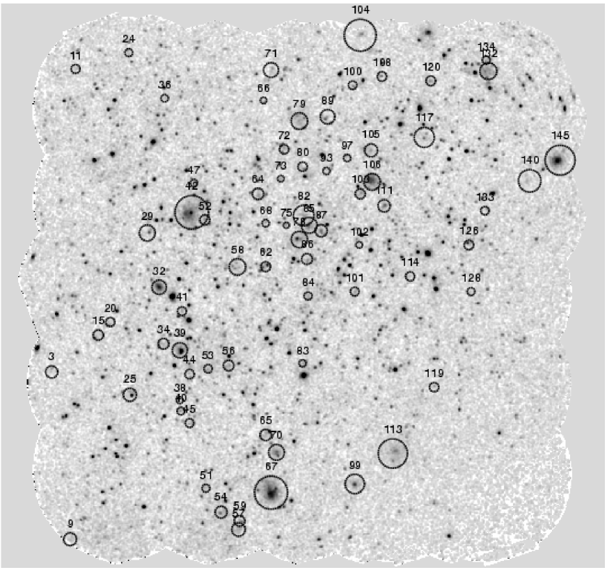
Figure 1.— An image of the signal-to-noise ratio in the 0.5–2 keV band, smoothed with a Gaussian of two pixel width. White color corresponds to values smaller than -0.5, while black corresponds to values exceeding 3. Circles indicate the position and size of the detected clusters, labeled in correspondence with the cluster number in the catalog. The image is 1.5 degrees on a side. The pixel size is $4^{\prime\prime}$ on a side. A tangential elongation in the point spread function of XMM-Newton telescopes is clearly visible in the NW corner of the image, which has the largest exposure time.

The paper is organized as follows: §2 describes the analysis of the XMM-Newton observations of the COSMOS survey; §3 presents our diffuse source detection technique; §4 describes the wavelet analysis of the photometric galaxy catalog; §5 provides the catalog of the identified X-ray groups and clusters of galaxies; §6 derives the luminosity function; and §7 concludes the paper.

2. XMM-COSMOS Data reduction

For cluster detection, we used the XMM-Newton mosaic image in the 0.5–2 keV band, based on the first 36 pointings of the XMM-Newton observations of the COSMOS field. The first 25 pointings completely cover the 2 square degree area of COSMOS at 57% of its final depth (Hasinger et al. 2007). 11 pointings have already been obtained as a part of the second year observations and are included in the present analysis. A description of the XMM-Newton observatory is given by Jansen et al. (2001). In this paper we use the data collected by the European Photon Imaging Cameras (EPIC): the pn-CCD camera (Strüder et al. 2001) and the MOS-CCD cameras (Turner et al. 2001). All Epic-pn observations have been performed using the Thin filter, while both Epic-MOS cameras used the Medium filter. An analysis of absolute frame registration for the XMM COSMOS survey has been carried out by Cappelluti et al. (2007). The offsets do not exceed $3^{\prime\prime}$ and do not affect the current analysis.

In addition to the standard data processing of the EPIC data, which was done using XMMSAS version 6.5 (Watson et al. 2001; Kirsch et al. 2004; Saxton et al. 2005), we perform a more conservative removal of time intervals affected by solar flares, following the procedure described in Zhang et al. (2004). In order to increase our capability of detecting extended, low surface brightness features, we have developed a sophisticated background removal technique, which we coin as ’quadruple background subtraction’, referring to the four following steps:

First, we remove from the image accumulation the photons in the energy band corresponding to the Al $K_{\alpha}$ line for pn and both MOS detectors and the Si $K_{\alpha}$ line for both MOS detectors. The resulting countrate-to-flux conversion in the 0.5–2 keV band excluding the lines is $1.59\times 10^{-12}$ for pn and $5.41\times 10^{-12}$ for each MOS detector, calculated for the source spectrum, corresponding to the APEC (Smith et al. 2001) model for a collisional plasma of 2 keV temperature, 1/3 solar abundance and a redshift of 0.2.

Second, we subtract the out-of-time events (OOTE) for pn. In order to do so, we generate an additional event file for each pn event file, which entirely consists of events emulating the OOTE, produced using the XMMSAS task epchain. We then apply the same selection of events using the good time intervals, generated during the light curve cleaning of the main event file. The last step is to extract the images with the same selection criteria (energy, flag, event pattern), normalize them by the fraction of OOTE (0.0629191 for the Full Frame readout mode used) and to subtract them from the main image.

Third and fourth, we use two known templates for the instrumental (unvignetted) and the sky (vignetted) background (Lumb et al. 2002, 2003). The instrumental background is caused by the energetic particles and has a uniform distribution over the detector. The sky background consists of the foreground galactic emission as well as unresolved X-ray background and its angular distribution on scales of individual observation could be considered as flat on the sky, therefore following the sensitivity map of the instrument (Lumb et al. 2002). To calculate the normalization for each template, we first perform a wavelet reconstruction (Vikhlinin et al. 1998b) of the image without a sophisticated background subtraction. We excise the area of the detector, where we detect flux on any wavelet scale and then split the residual area into two equal detector parts with higher and lower values of vignetting than the median value. By imposing a criterion that the weighted sum of the two templates should reproduce the counts in both areas, we obtain a system of two linear equations for two weighting coefficients. By solving the latter we derive the best estimate for the normalizations of both templates.

After the background has been estimated for each observation and each instrument separately, we produce the final mosaic of cleaned images and correct it for the mosaic of the exposure maps in which we account for differences in sensitivity between pn & MOS detectors stated above. The detailed treatment of the background is newly developed and has been adopted for all XMM-COSMOS projects (Cappelluti et al. 2007). The procedure of mosaicing of XMM-Newton data has been used previously and is described in detail in Briel et al. (2004).

The resulting signal-to-noise ratio image is shown in Fig. 1. As can be seen from the figure, the image exhibits a fairly uniform signal-to-noise ratio. Without the refined background subtraction, the signal-to-noise image exhibited large-scale variations, which could mimic an extended source. On the image, the circles show the position and the angular extent of detected clusters of galaxies. The pixel size of the X-ray images employed in the current analysis is $4^{\prime\prime}$ on a side.

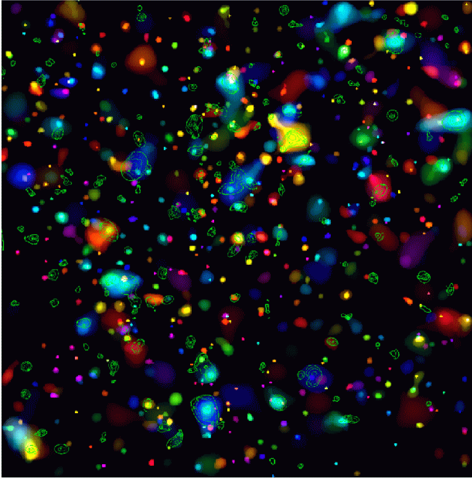
Figure 2.— The colors of COSMOS. The wavelet reconstruction of the early-type galaxy concentrations searched in the photo-z catalog is color-coded according to the average redshift: blue – 0.2, cyan – 0.4, green – 0.6, yellow – 0.8, red – 1.0. The green contours outline the area of the X-ray emission associated with 150 extended source candidates. The image is 1.5 degrees on a side. The pixel size is $10^{\prime\prime}$ on a side.

3. Cluster detection technique

We used the wavelet scale-wise reconstruction of the image, described in Vikhlinin et al. (1998b), employing angular scales from $8^{\prime\prime}$ to $2.1^{\prime}$. We apply the approach of Rosati et al. (1998), Vikhlinin et al. (1998b), and Moretti et al. (2004) to effectively select clusters of galaxies by the spatial extent of their X-ray emission. The cluster detection algorithm consists of two parts: (1) selection of the area with detectable flux on large angular scales, and (2) removal of the area where the flux could be explained by contamination from embedded point-like sources, most of which are background AGNs, according to their optical identification (Brusa et al. 2007). When applying this approach to XMM-Newton data, the off-axis behavior of the point-spread function (PSF) (e.g. Valtchanov et al. 2001) needs to be taken into account. The major change in the two-dimensional shape of the PSF of the XMM telescope is a tangential elongation with respect to the optical axis of the telescope (Lumb et al. 2003). In the wavelet scale-wise reconstruction of the point source, this produces a flux redistribution between the $8^{\prime\prime}$ and $16^{\prime\prime}$ scales with more flux going into the $16^{\prime\prime}$ at large off-axis angles. At the same time, the flux contained in the sum of $8^{\prime\prime}$ and $16^{\prime\prime}$ wavelet scales does not vary much with the off-axis angle and its ratio to the flux detected on larger angular scales is greater than 1.9 at any off-axis angle. Smaller flux ratios have therefore been chosen as a detection criterion for an extended source.

Our wavelet algorithm (Vikhlinin et al. 1998b) generates a noise map against which the flux in the image is tested for significance. We assess the sensitivity of the survey, by examining the noise map corresponding to the $32^{\prime\prime}$ scale. The total area over which the source of a given flux can be detected is the area where the source signal to noise ratio exceeds the chosen detection threshold of 4. For each cluster this number is unique, yet the total flux of the cluster is not recovered at $32^{\prime\prime}$. Any procedure to recover the total flux introduces a scatter in the total flux vs survey area relation. The noise map is calculated using the data, and so it includes the effect of decreasing sensitivity to a diffuse source detection caused by the contamination from other X-ray sources. Our calculation of the sensitivity neglects cluster-cluster and cluster-point source correlations. In this regard, a presence of an unresolved bright cool core could complicate the detection of a cluster. A modelling of such effect will be done within the granted C-COSMOS program.

The source appearance on the $32^{\prime\prime}$ wavelet scale defines the area which is further used for measuring the parameters of the source. The total flux of the source is obtained by extrapolation of the flux measured within this area. As a first step in selecting the cluster candidates, we clean our source list from contamination due to point sources. For that, we compare the sum of the two smallest scales ($8^{\prime\prime}$ and $16^{\prime\prime}$) with the sum of the largest scales ($32^{\prime\prime}$, $64^{\prime\prime}$, $128^{\prime\prime}$) in the same area to decide whether the area contains a diffuse source. If the sum of the two smallest scales exceeds the sum of the three largest scales by a factor of 1.9 or greater, the source is removed from the diffuse source list. This procedure allows us to deal with any number of point sources embedded in the same area. We find that 80% of the initially selected areas are dominated by the flux from point sources. Out of the remaining 150 diffuse source candidates, surviving this test, we identify only 76 with peaks in the galaxy distribution, as detailed in §4. The bulk of unidentified sources are confused low-luminosity AGNs, which are not detected on the small scales. Some of those sources might be identified by chance with a galaxy overdensity. The probability of such event is 1%, as determined by the fraction of the total XMM-COSMOS area occupied by the unidentified sources, which were initially considered as extended source candidates. Sect. 4 describes the construction of the catalog of 420 galaxy groups based on the multiband photometric data. The number of optical peaks missing identification with an extended X-ray source is 345, leading to a chance identification for $\sim 3$ clusters. The misidentifications have large separations between the X-ray center and the optical center of a group, as a chance coincidence of the centers is negligibly small. So, through a comparison to optical images we removed 4 sources whose shape of X-ray emission was not associated with a group of galaxies, finally reducing the cluster sample size to 72. For all four rejected systems, one can decompose the emission into 3-5 unresolved AGN using the K-band images identification, similar to the primary method for AGN identification used in the COSMOS field (Brusa et al. 2007).

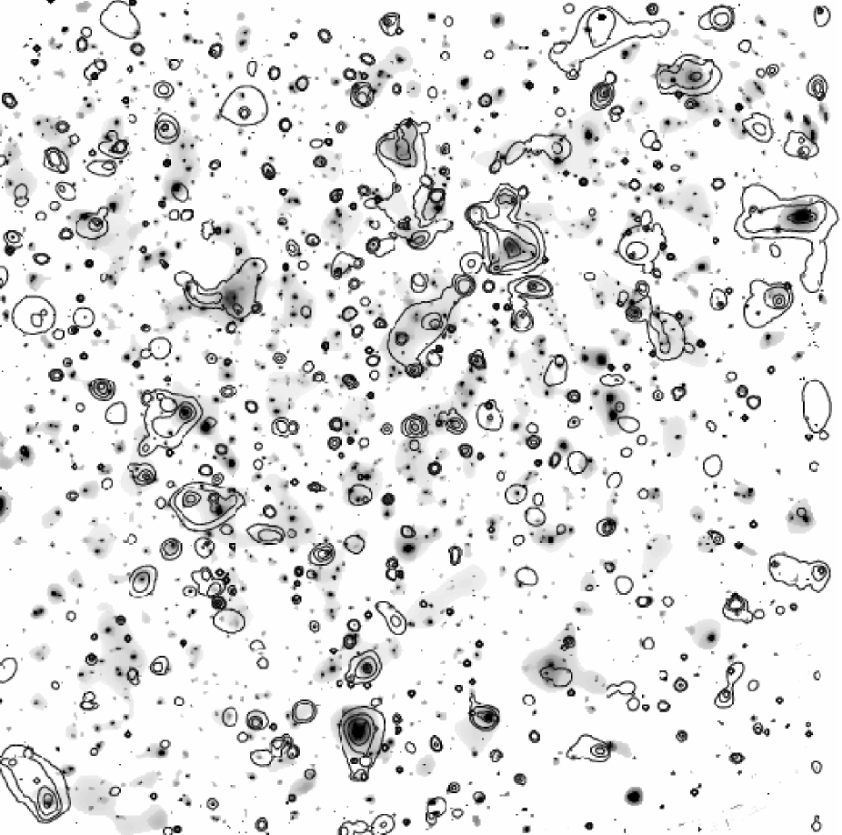
Figure 3.— Scale-wise wavelet reconstruction of the XMM-COSMOS mosaic image in the 0.5–2 keV band. Grey color corresponds to the surface brightness of $10^{-7}$ counts s^-1 pixel^-1. A surface brightness level exceeding $10^{-5}$ counts s^-1 pixel^-1 is shown in black. Contours indicate the location and strength of galaxy structures, identified in the photo-z catalog. The image is 1.5 degrees on a side. The pixel size is $4^{\prime\prime}$ on a side.

It is possible to reduce the number of spurious X-ray detections. However, it would result in a loss of survey sensitivity (Vikhlinin et al. 1998b) and is usually done to improve the efficiency of the optical follow-up. Since such a follow-up already exists in the COSMOS field, we prefer to keep the high sensitivity achieved by our detection method.

Although some additional flux is detected on larger scales, the source confusion becomes large on scales exceeding $1^{\prime}$ at the flux limits typical of our survey. In addition, the use of only a single scale for the detection has the advantage of allowing a more straight-forward modeling.

Once a diffuse source is detected, the next step is to estimate its total flux. Unlike in the case of point sources, this is complicated by the unknown shape of a diffuse source. For bright sources, it is possible to carry out a surface brightness analysis and estimate the missing flux directly. For example, an analysis of the surface brightness profile for a bright cluster at $z=0.22$ in COSMOS using the beta model (Smolčić et al. 2007) results in a factor of 1.8 higher flux compared to the total flux within the aperture defined by the source detection procedure.

Studies of nearby clusters of galaxies (e.g. Markevitch 1998) show that most of the cluster flux is encompassed within the radius $r_{500}$ (a radius encompassing the matter density 500 times the critical), so we adopt this radius for the total flux measurements, $F(<r_{500})$. We have therefore adopted a method for estimating $r_{500}$, based on the iteratively corrected observed flux

$$F(<r_{500})=C_{\beta}(z,T)F_{\rm d}$$ (1)

with the correction, $C_{\beta}(z,T)$, defined iteratively through the scaling relations as described in §5.1 and using the flux and redshift of the system. To estimate the observed flux we use the total counts ($F_{\rm d}$) in the area defined by the detection algorithm ($R_{\rm t}$) and subtract the contribution from the embedded point sources based on intensity determined by the $4^{\prime\prime}$ scale ($R_{4^{\prime\prime}}$) of the wavelet. The total flux retained in the area is larger than $R_{4^{\prime\prime}}$ by a factor, determined by the size of the area ($a$) and the XMM PSF ($C_{\rm PSF}(a)$), with values in the range 1.1–1.5. We work in units of MOS1 counts/s on the mosaic. We add pn and MOS counts as observed, while putting more effective weight to the pn exposure map, so that

$$F_{\rm d}=5.41\times 10^{-12}(R_{\rm t}-C_{\rm PSF}(a)\times R_{4^{\prime\prime}}){\rm ergs\;s}^{-1}{\rm cm}^{-2}$$ (2)

Also, after removal of cool cores, the scatter in the scaling relations is found to be moderate (Markevitch et al. 1998; Finoguenov et al. 2005a). In our survey, a cool core is indistinguishable from an AGN and is therefore removed from the flux estimates.

As has been described above, the area for cluster flux extraction has been selected based on a particular ($32^{\prime\prime}$) spatial scale. Thus, only a part of the cluster emission is used in the detection. This results in an effective loss of sensitivity, as not all the cluster emission is used. However, the modeling of the detection becomes simple and in particular, an influence of the cool cluster cores on the cluster detection statistics is reduced.

4. Use of photometric redshifts to identify the clusters

The identification/confirmation of a bound galaxy system would be most robust through optical/NIR spectroscopic redshift measurement, but this is costly for such a large survey. Photometric redshifts, when measured with sufficient accuracy, represent a viable alternative. The COSMOS survey, providing both the photo-z (Mobasher et al. 2007) and in the future the spectral-z (Lilly et al. 2007) is an ideal field to understand all the pros and cons of the use of photo-z to identify the optical counterparts to X-ray clusters. Diffuse X-ray emission, associated with a galaxy overdensity, is by itself a proof of the virialized nature of the object (Ostriker et al. 1995), so a combination of diffuse X-ray source and a photo-z galaxy overdensity validates the photo-z source as a virialized object. Deep multiband photometric observations have been carried out in the COSMOS field using CFHT, Subaru, CTIO and KPNO facilities (Capak et al. 2007). The combination of depth and bands allows us to produce an $i$-band based photo-z catalog with a $1\sigma$ uncertainty of the redshift estimate of $0.027(1+z)$ for galaxies with $i_{AB}<25$ (Mobasher et al. 2007) obtained without the luminosity prior. While both z and K-band data are used in determining the photometric redshifts, the input catalog is based on the $i$-band images. Therefore, the redshift range of the cluster search in this paper has to be limited to redshifts below 1.3, after which the 4000Å break moves redward of the $i$-band filter.

To provide an identification of galaxy overdensities in the photo-z space, we select from the original photo-z catalog only the galaxies, that (1) are classified in their SED (spectral energy distribution) as early-types (ellipticals, lenticulars and bulge-dominated spirals); (2) have high quality photo-z redshift determination (95% confidence interval for the redshift determination is lower than $\Delta z=0.4$); (3) are not morphologically classified as stellar objects. Given the current quality of photo-z, we select redshift slices covering the range $0<z<1.3$ with both $\Delta z=0.1$ and $\Delta z=0.2$. To provide a more refined redshift estimate for the identified structures, we slide the selection window with a 0.05 step in redshift. We add each galaxy as one count and apply wavelet filtering (Vikhlinin et al. 1998b) to detect enhancements in the galaxy number density on scales ranging from 20^′′ to 3^′ on a confidence level of $4\sigma$ with respect to the local background. The local background itself is determined by both the field galaxies located in the same redshift slice as well as galaxies attributed to the slice due to a catastrophic failure in the photo-z. The fraction of galaxies assigned to structures in our analysis varies from 15% at a $z=0.3$ to 2% at $z=1.2$. However, the level of the background does not vary strongly with redshift, so the detection of the optical counterpart is primarily determined by the sensitivity, required to determine the photometric redshift for sufficient number of members. As will be discussed below, the X-ray detection limits at $z>1$ in the COSMOS survey correspond to a massive cluster, that typically has a sufficient number of bright members, enabling the success of the identification procedure.

The angular scales selected for the analysis match the extent of X-ray sources found. While the number of galaxies within each cluster is not determined by the statistics, our ability to see it over the background is statistical with the errors determined by the background level. Analysis of galaxy overdensities is not sensitive to catastrophic failures in the photo-z catalog, as those simply reduce the strength of galaxy concentration. Larger structures, selected without the prior on the SED type, are reported in Scoville et al. (2007b) and should be understood as the LSS environment within which the high-density peaks detected via X-ray emission are located. Making a prior on SED type is technically necessary to increase the contrast in the photometric data. From a theoretical point of view, the use of these specific SEDs is justified by the large ages of cluster ellipticals and the lack of evolution in their morphological fraction with redshift (Smith et al. 2005; Postman et al. 2005; Wechsler et al. 2005; see also direct estimates from the COSMOS field in Capak et al. 2007 and Guzzo et al. 2007), where the already tested redshift range reaches $z=1.1$ (Hashimoto et al. 2005). The ultra-deep field of the UKIRT Infrared Deep Sky Survey (Lawrence et al. 2006) finds that the galaxy red sequence disappears beyond $z=1.5$ (Cirasuolo et al. 2006). Moreover, local spiral-rich groups also do not reveal X-ray emission associated with their IGM (Mulchaey et al. 1996). In §6 we verify the completeness of the source identification using the $V/V_{max}$ test and conclude that we do not lack high-redshift identification in our analysis. In comparison with the widely adopted cluster red sequence method, the use of photo-z data allows us to include fainter members, which is of particular importance for galaxy groups.

Table 1Catalog of the identified X-ray clusters.

	R.A	Decl.	$r_{500}$	flux $10^{-14}$	z	M500	L0.1-2.4keV	kT	z
ID	Eq.2000		$\prime$	ergs cm-2 s-1		$10^{13}$ M⊙	$10^{42}$ ergs s-1	keV	source
3	150.80244	1.98985	1.0	$0.70\pm 0.16$	0.25	$0.69\pm 0.14$	$2.2\pm 0.5$	$0.56\pm 0.06$	1
9	150.75121	1.52793	1.1	$1.97\pm 0.38$	0.75	$9.62\pm 1.65$	$75.4\pm 14.5$	$2.62\pm 0.23$	1
11	150.73676	2.82680	0.7	$0.40\pm 0.08$	0.60	$1.88\pm 0.35$	$10.2\pm 2.1$	$1.06\pm 0.10$	1
15	150.67342	2.09190	0.9	$0.50\pm 0.09$	0.34	$0.88\pm 0.13$	$3.2\pm 0.5$	$0.65\pm 0.05$	0
20	150.64041	2.12791	0.8	$0.43\pm 0.06$	0.55	$1.78\pm 0.23$	$9.0\pm 1.3$	$1.01\pm 0.07$	1
24	150.58962	2.87187	0.7	$0.36\pm 0.08$	0.95	$3.41\pm 0.66$	$30.6\pm 6.6$	$1.61\pm 0.16$	1
25	150.58631	1.92693	1.1	$1.04\pm 0.10$	0.30	$1.36\pm 0.12$	$4.9\pm 0.5$	$0.81\pm 0.04$	1
29	150.53842	2.37393	1.3	$1.28\pm 0.15$	0.18	$0.62\pm 0.07$	$1.8\pm 0.2$	$0.52\pm 0.03$	0
32	150.50535	2.22395	1.2	$3.45\pm 0.11$	0.90	$18.64\pm 0.52$	$189.7\pm 5.9$	$3.90\pm 0.06$	1
34	150.49330	2.06795	0.9	$0.61\pm 0.07$	0.40	$1.47\pm 0.14$	$6.0\pm 0.6$	$0.87\pm 0.04$	1
36	150.49048	2.74592	0.6	$0.22\pm 0.05$	0.65	$1.34\pm 0.30$	$7.4\pm 1.9$	$0.90\pm 0.10$	1
38	150.44824	1.91197	0.6	$0.26\pm 0.04$	1.25	$3.49\pm 0.50$	$45.1\pm 7.3$	$1.79\pm 0.13$	1
39	150.44827	2.04996	1.3	$2.54\pm 0.13$	0.55	$8.10\pm 0.38$	$48.4\pm 2.5$	$2.25\pm 0.05$	1
40	150.44523	1.88197	0.6	$0.26\pm 0.04$	0.70	$1.70\pm 0.23$	$10.4\pm 1.6$	$1.03\pm 0.07$	1
41	150.44229	2.15796	0.7	$0.30\pm 0.06$	0.40	$0.77\pm 0.13$	$3.0\pm 0.6$	$0.62\pm 0.05$	1
42	150.41533	2.43096	2.8	$11.45\pm 0.26$	0.12	$2.26\pm 0.05$	$7.1\pm 0.2$	$1.01\pm 0.01$	0
44	150.42124	1.98397	0.8	$0.42\pm 0.07$	0.45	$1.26\pm 0.19$	$5.4\pm 0.9$	$0.81\pm 0.06$	1
45	150.42121	1.84898	0.7	$0.49\pm 0.05$	0.85	$3.70\pm 0.35$	$29.5\pm 3.1$	$1.63\pm 0.08$	1
47	150.40934	2.51196	0.6	$0.29\pm 0.04$	1.00	$2.97\pm 0.34$	$27.9\pm 3.5$	$1.52\pm 0.09$	1
51	150.37616	1.66900	0.7	$0.32\pm 0.04$	0.75	$2.20\pm 0.28$	$14.6\pm 2.1$	$1.20\pm 0.08$	1
52	150.37930	2.40997	0.8	$0.47\pm 0.06$	0.35	$0.87\pm 0.10$	$3.1\pm 0.4$	$0.65\pm 0.04$	0
53	150.37021	1.99898	0.7	$0.41\pm 0.05$	0.85	$3.20\pm 0.34$	$25.2\pm 3.0$	$1.51\pm 0.08$	1
54	150.33413	1.60301	1.0	$0.88\pm 0.10$	0.40	$2.03\pm 0.20$	$8.6\pm 0.9$	$1.03\pm 0.05$	1
56	150.31318	2.00799	0.9	$0.57\pm 0.07$	0.35	$1.03\pm 0.11$	$3.8\pm 0.4$	$0.71\pm 0.04$	1
57	150.28611	1.55502	1.1	$1.27\pm 0.13$	0.36	$2.26\pm 0.20$	$9.3\pm 0.9$	$1.08\pm 0.05$	0
58	150.28916	2.28024	1.4	$0.91\pm 0.10$	0.12	$0.27\pm 0.03$	$0.7\pm 0.1$	$0.32\pm 0.02$	0
59	150.28311	1.57902	0.9	$0.62\pm 0.10$	0.36	$1.18\pm 0.17$	$4.5\pm 0.7$	$0.77\pm 0.06$	0
62	150.21114	2.28100	0.8	$0.79\pm 0.06$	0.88	$5.65\pm 0.37$	$49.1\pm 3.6$	$2.06\pm 0.07$	0
64	150.23218	2.48199	0.9	$0.64\pm 0.06$	0.30	$0.88\pm 0.08$	$3.0\pm 0.3$	$0.64\pm 0.03$	1
65	150.21111	1.81600	0.9	$0.89\pm 0.07$	0.53	$3.16\pm 0.23$	$16.6\pm 1.4$	$1.36\pm 0.05$	0
66	150.21718	2.73998	0.5	$0.15\pm 0.04$	0.95	$1.81\pm 0.45$	$15.2\pm 4.3$	$1.16\pm 0.15$	1
67	150.19609	1.65701	2.7	$17.94\pm 0.30$	0.22	$10.11\pm 0.15$	$41.6\pm 0.7$	$2.29\pm 0.02$	0
68	150.21115	2.40100	0.6	$0.24\pm 0.04$	0.90	$2.40\pm 0.34$	$19.5\pm 3.1$	$1.32\pm 0.10$	1
70	150.18109	1.76801	1.3	$2.09\pm 0.11$	0.35	$3.27\pm 0.15$	$13.7\pm 0.7$	$1.31\pm 0.03$	0
71	150.19616	2.82397	1.2	$1.14\pm 0.21$	0.20	$0.70\pm 0.12$	$2.1\pm 0.4$	$0.55\pm 0.05$	1
72	150.16011	2.60499	0.8	$0.69\pm 0.07$	0.90	$5.34\pm 0.47$	$47.4\pm 4.6$	$2.02\pm 0.09$	1
73	150.16912	2.52400	0.5	$0.15\pm 0.03$	0.75	$1.24\pm 0.22$	$7.7\pm 1.6$	$0.89\pm 0.08$	1
75	150.15410	2.39500	0.5	$0.16\pm 0.03$	1.15	$2.23\pm 0.34$	$24.4\pm 4.2$	$1.37\pm 0.11$	1
78	150.11807	2.35600	1.3	$1.74\pm 0.11$	0.22	$1.19\pm 0.07$	$3.8\pm 0.2$	$0.74\pm 0.02$	0
79	150.11807	2.68299	1.4	$2.46\pm 0.19$	0.35	$3.84\pm 0.26$	$16.5\pm 1.2$	$1.42\pm 0.05$	0
80	150.10906	2.55700	0.8	$0.44\pm 0.07$	0.50	$1.56\pm 0.21$	$7.3\pm 1.1$	$0.93\pm 0.06$	1
82	150.10606	2.42200	1.0	$0.76\pm 0.07$	0.22	$0.59\pm 0.05$	$1.8\pm 0.2$	$0.51\pm 0.02$	0
83	150.10906	2.01400	0.6	$0.25\pm 0.04$	0.85	$2.09\pm 0.31$	$15.6\pm 2.6$	$1.21\pm 0.09$	0
84	150.09405	2.20000	0.7	$0.36\pm 0.04$	0.93	$3.29\pm 0.34$	$28.5\pm 3.3$	$1.57\pm 0.08$	0
85	150.09105	2.39500	1.3	$1.58\pm 0.10$	0.22	$1.10\pm 0.06$	$3.5\pm 0.2$	$0.71\pm 0.02$	0
86	150.09705	2.30200	0.9	$0.63\pm 0.06$	0.36	$1.18\pm 0.10$	$4.5\pm 0.4$	$0.76\pm 0.04$	0
87	150.05802	2.38000	1.0	$0.91\pm 0.08$	0.40	$2.08\pm 0.16$	$8.8\pm 0.7$	$1.04\pm 0.04$	1
89	150.03999	2.69499	1.2	$1.04\pm 0.14$	0.20	$0.66\pm 0.08$	$2.0\pm 0.3$	$0.54\pm 0.03$	1
93	150.04300	2.54500	0.6	$0.34\pm 0.05$	1.25	$4.15\pm 0.56$	$54.6\pm 8.2$	$1.96\pm 0.13$	1
97	149.98594	2.58099	0.6	$0.21\pm 0.04$	0.70	$1.43\pm 0.24$	$8.5\pm 1.6$	$0.94\pm 0.08$	1
99	149.96500	1.68101	1.6	$4.38\pm 0.26$	0.37	$7.05\pm 0.38$	$33.3\pm 2.0$	$1.98\pm 0.06$	0
100	149.97091	2.78197	0.7	$0.39\pm 0.07$	0.70	$2.37\pm 0.39$	$15.0\pm 2.7$	$1.23\pm 0.10$	1
101	149.96495	2.21199	0.7	$0.31\pm 0.05$	0.43	$0.89\pm 0.13$	$3.5\pm 0.6$	$0.67\pm 0.05$	0
102	149.95293	2.34099	0.5	$0.20\pm 0.03$	1.10	$2.60\pm 0.38$	$27.1\pm 4.4$	$1.46\pm 0.11$	1
103	149.94991	2.48199	0.8	$0.84\pm 0.08$	0.80	$5.31\pm 0.46$	$41.5\pm 4.0$	$1.95\pm 0.09$	1
104	149.94987	2.91995	2.7	$9.96\pm 0.98$	0.13	$2.08\pm 0.18$	$6.5\pm 0.6$	$0.97\pm 0.04$	0
105	149.91987	2.60198	1.1	$0.88\pm 0.08$	0.25	$0.84\pm 0.07$	$2.7\pm 0.2$	$0.62\pm 0.03$	1
106	149.91688	2.51498	1.4	$4.56\pm 0.13$	0.73	$18.90\pm 0.48$	$155.7\pm 4.4$	$3.73\pm 0.05$	0
108	149.88981	2.80596	0.8	$0.53\pm 0.09$	0.65	$2.82\pm 0.41$	$17.0\pm 2.8$	$1.33\pm 0.10$	1
111	149.88386	2.44898	1.0	$0.96\pm 0.09$	0.36	$1.70\pm 0.13$	$6.8\pm 0.6$	$0.93\pm 0.04$	0
113	149.85995	1.76499	2.4	$7.44\pm 0.44$	0.12	$1.55\pm 0.08$	$4.6\pm 0.3$	$0.83\pm 0.02$	0
114	149.81183	2.25397	0.8	$0.39\pm 0.07$	0.47	$1.29\pm 0.21$	$5.7\pm 1.0$	$0.83\pm 0.07$	0
117	149.77272	2.63795	1.7	$1.03\pm 0.17$	0.08	$0.14\pm 0.02$	$0.3\pm 0.1$	$0.23\pm 0.02$	0
119	149.74586	1.94797	0.8	$0.41\pm 0.09$	0.45	$1.22\pm 0.24$	$5.2\pm 1.1$	$0.80\pm 0.08$	1
120	149.75467	2.79393	0.8	$0.50\pm 0.06$	0.49	$1.70\pm 0.18$	$8.0\pm 0.9$	$0.97\pm 0.05$	0
126	149.64969	2.34093	0.8	$0.87\pm 0.10$	1.00	$6.87\pm 0.69$	$70.8\pm 7.9$	$2.37\pm 0.12$	1
128	149.64372	2.21193	0.6	$0.38\pm 0.09$	1.00	$3.63\pm 0.75$	$34.8\pm 8.1$	$1.69\pm 0.18$	1
132	149.59548	2.82087	1.4	$2.57\pm 0.13$	0.34	$3.92\pm 0.18$	$16.8\pm 0.9$	$1.44\pm 0.04$	1
133	149.60532	2.43541	0.7	$0.57\pm 0.07$	1.15	$5.68\pm 0.64$	$68.7\pm 8.6$	$2.25\pm 0.13$	1
134	149.60148	2.85087	0.6	$0.34\pm 0.05$	0.95	$3.26\pm 0.46$	$29.1\pm 4.6$	$1.58\pm 0.11$	1
140	149.48149	2.51785	1.9	$2.04\pm 0.32$	0.09	$0.31\pm 0.04$	$0.7\pm 0.1$	$0.35\pm 0.03$	0
145	149.39739	2.57480	2.5	$20.42\pm 0.46$	0.37	$26.47\pm 0.54$	$144.9\pm 3.3$	$3.98\pm 0.04$	0

In Fig. 2 we overlay the X-ray contours of diffuse sources over the color-coded image of the structures identified via the photo-z galaxy selection. The brightness of the color is proportional to the number density of galaxies, while the color represents the average redshift. In addition, to show the correspondence between galaxy structures and X-ray emission, we provide in Fig. 3 an overlay of the wavelet-reconstructed X-ray image with the contours, showing the sum of the wavelet-filtered redshift galaxy slices.

To determine the redshift of an X-ray structure, we calculate the position and maximum of the galaxy density peak using the photo-z slices. The extended source candidate is considered identified as a cluster if it contains a galaxy density peak inside the detected extend, which is typically $20^{\prime\prime}-40^{\prime\prime}$. The redshift and center of the cluster is selected to be associated with the strongest galaxy peak inside the cluster. Due to the wings in the redshift estimate using the photometric technique, the cluster is detected over a range of redshifts. Selecting the peak value is thought to yield the most likely redshift of the cluster. In the case of several overlapping structures, this could lead to biases due to redshift selection effects and in any case should be verified. In one instance (cluster 133), we manually put a preference for a high redshift counterpart, which matched both the X-ray center and the redshift of BCG of the system. In total, 72 X-ray clusters have been identified using this method. Their properties are listed in Tab. 1 and discussed below.

5. A catalog of identified X-ray clusters

In this section we describe our catalog of 72 X-ray galaxy clusters detected so far in the COSMOS field. In the catalog we provide the cluster identification number (column 1), R.A. and Decl. of the peak of the galaxy concentration identified with the extended X-ray source in Equinox J2000.0 (2–3), the estimated radius $r_{500}$ in arcminutes (4), the cluster flux in the 0.5–2 keV band within $r_{500}$ in units of $10^{-14}$ ergs cm^-2 s^-1 with the corresponding 1 sigma errors (5), photometric redshift (6), an estimate of the cluster mass, $M_{500}$, in units of $10^{13}M_{\odot}$ (7), rest-frame luminosity in the 0.1–2.4 keV band (8), an estimate of the IGM temperature in keV (9), the source of redshift (10) with 1 denoting the photometric redshift estimates and 0 denoting the redshift refinement using information available from the SDSS DR4 (York et al. 2000, Abazajian et al. 2005; Adelman-McCarthy et al. 2006), the results of the pilot zCOSMOS program, and the first results of the main zCOSMOS program (Lilly et al. 2007). The refinement of the photo-z is complete for $z<0.2$, which reduces the degree of uncertainty in calculation of distance-dependent properties of the sample to a level, well within the scatter in the scaling relations for X-ray clusters (e.g. Stanek et al. 2005). The formal error on the positional uncertainty is of the order of $10^{\prime\prime}$. The errors provided on the derived properties are only statistical. A future study of systematic errors will be done by direct comparison between our reported mass estimates and the weak lensing measurements (Leauthaud et al., in prep.; Taylor et al., in prep.). For a number of clusters with best X-ray statistics, it appears that the peak of the galaxy density can be somewhat offset from the X-ray center, which in turn has a better match with the position of the brightest cluster galaxy. Further investigation of this interesting property will be done elsewhere.

In order to calculate the properties of the clusters, we use the known scaling relations at low-redshift and evolve them according to the recent Chandra and XMM observations of high-redshift clusters of galaxies (Kotov & Vikhlinin 2005; Finoguenov et al. 2005b; Ettori et al. 2004; Maughan et al. 2006). Following Evrard et al. (2002), we choose not to correct for the redshift evolution of the ratio of the density encompassed by the cluster virial radius to the critical density.

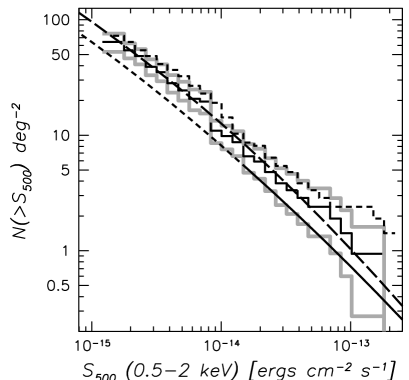
Figure 4.— Left panel: Cumulative cluster number counts ($\log(N>S)-\log(S)$) for the COSMOS field. The solid histogram shows the data and grey histograms denote the 68% confidence interval. The black solid/short-dashed curve shows the results of the modeling of RDCS (Rosati et al. 2002), with the solid part corresponding to fluxes sampled by their data, while the short dashed line denotes the model prediction. The long dashed curve shows the prediction for no evolution in the luminosity function in Rosati et al. (2002), which provides a good fit to our data. The dashed histogram shows a typical difference due to assumption of the scaling relations. Right panel: Survey area as a function of the total source flux in the 0.5–2 keV band. Open circles show the area corresponding to the source, while the solid line shows the sensitivity curve for the flux in the detection cell, scaled up to match the displayed data. The scatter of points around the curve is determined by differences in the flux losses between distant and nearby sources.

5.1. Flux estimates

Even a basic statistical description of the cluster sample, such as $\log(N)-\log(S)$, is not entirely straight-forward, as it requires a knowledge of the level of the emission at large distances from the cluster center. Most cluster surveys to date either use much deeper reobservation of the clusters for this purpose or extrapolate the detected cluster flux assuming some model for the spatial shape of the emission. Although most observers agree that the $\beta$-model (Jones & Forman 1984; 1999) is a good description of the cluster shape, characterization of the outskirts of groups and clusters of galaxies is still uncertain (e.g. Vikhlinin et al. 2006; Borgani et al. 2004). Moreover, groups reveal a large scatter in the shape of their emission (Finoguenov et al. 2001; Mahdavi et al. 2005).

For the purpose of this paper, we extrapolate the measured flux ($F_{\rm d}$) by an amount of $C_{\beta}(z,T)$, which uses the $\beta$-model characterization of cluster emission, with the following parameters

$$\beta=0.4\times({kT/1{\rm keV}})^{1/3}$$ (3)

and

$$r_{\rm core}=0.07\times({kT/1{\rm keV}})^{0.63}\times r_{500}$$ (4)

We note that although the cool core clusters require a second spatial component to describe the central peak of their emission, in our case the contribution of a cool core cannot be distinguished from point sources and has therefore been removed from the flux estimates. Since only the large-scale component exhibits a scaling with temperature (Markevitch 1998), removal of the center should result in reduced scatter in the derived cluster characteristics, such as the total mass. More importantly, exclusion of cool cores from the detection procedure decreases an observational bias towards low-mass groups with strong cool cores, and make a selection of the sample to be closer to mass selection, and reduces the bias discussed in Stanek et al. (2006) and O’Hara et al. (2006), while facilitating the modelling of the cluster detection. However, subtle differences in the derived characteristics of the sample are expected as discussed below. In calculating the rest-frame luminosity, we iteratively use the total flux within an estimated $r_{500}$ ($C_{\beta}(z,T)F_{\rm d}$) and apply the K-correction ($K(z,T)$) accounting for the temperature and redshift of the source, following the approach described in Böhringer et al. (2004) and assuming an element abundance of 1/3 solar. So, finally, the derived luminosity is

$$L_{0.1-2.4\rm keV}=4\pi d_{L}^{2}K(z,T)C_{\beta}(z,T)F_{\rm d}$$ (5)

We note that a similar approach for reconstructing the cluster flux is taken in Henry et al. (1992), Nichol et al. (1997), Scharf et al. (1997), Ebeling et al. (1998), Vikhlinin et al. (1998b), de Grandi et al. (1999), Reprich & Böhringer (2002), and Böhringer et al. (2004). A choice of $r_{500}$ as a limiting radius is motivated by the results of Vikhlinin et al. (2006) on the steepening in the surface brightness profiles, observed near this radius.

To estimate the temperature of each cluster, we use the $L_{0.1-2.4\rm keV}-T$ relations of Markevitch (1998) for the case of excised cool cores:

$$kT=6\;{\rm keV}\times 10^{(\log_{10}(L_{0.1-2.4\rm keV}E_{z}^{-1})-44.45)/2.1)}$$ (6)

where

$$E_{z}=(\Omega_{M}(1+z)^{3}+\Omega_{\Lambda})^{1/2}$$ (7)

The estimates of the total gravitational mass and the corresponding $r_{500}$ are performed using the M–T relation (F. Pacaud 2005, private communication) re-derived from Finoguenov et al. (2001) using an orthogonal regression and correcting the masses to $h_{70}$ and a $\Lambda$CDM cosmology:

$$M_{500}=2.36\times 10^{13}M_{\odot}\times T^{1.89}E_{z}^{-1}$$ (8)

and

$$r_{500}=0.391\,{\rm Mpc}\times(kT/{\rm keV})^{0.63}E_{z}^{-1}$$ (9)

Although the $L_{500}-T$ relation of Markevitch (1998) is formally derived for high-temperature clusters, a comparison of that relation with the new results on the $L_{500}-T$ relation for groups (Ponman T.J., private communication), shows that the two are very similar. Based on direct comparison between the predicted and measured temperatures for a number of clusters in the COSMOS (e.g. Smolčić et al. 2007; Guzzo et al. 2007), the mass estimates provided in Tab. 1 should be good to a factor of 1.4, due to both the scatter in the scaling relations and uncertainty in our knowledge of their redshift evolution.

5.2. Cluster counts

It is common to characterize a cluster survey by its area as a function of the limiting flux and present the results as a relation between a cumulative surface density of clusters above a given flux limit vs the flux value, the cluster $\log(N>S)-\log(S)$ (e.g. Rosati et al. 1998). In order to take into account the difference between the total flux and the observed flux, the $\log(N>S)-\log(S)$ is computed by assigning to each cluster a weight equal to the inverse value of the area for its observed flux. Such area-flux relation is determined by the wavelet detection algorithm and is therefore known precisely. This weight is further added to the flux bin in correspondence to the total flux of the cluster.

While the calculation of the survey area as a function of cluster flux in the detection cell is exact, the survey area as a function of total cluster flux is known only approximately and exhibits a scatter, as illustrated in the right panel of Fig. 4. Lower redshift systems require more extrapolation for a given flux in the detection cell. Similarly, within the same redshift range, more massive systems require larger degree of flux extrapolation given the fixed size of the detection cell.

The left panel of Fig. 4 shows the $\log(N>S)-\log(S)$ relation of the COSMOS field clusters. Although with a somewhat higher normalization, the COSMOS $\log(N>S)-\log(S)$ is statistically consistent with RDCS results of Rosati et al. (2002) for the fluxes $S>10^{-14}$ ergs cm^-2 s^-1. While a similarly higher normalization of the $\log N-\log S$ has also been reported for the XMM-LSS survey (Pierre et al. 2005) as well as for the 160 square degrees survey (Vikhlinin et al. 1998b), an important difference between those surveys and the RDCS consists in extrapolation of the cluster flux beyond the detection radius. As no extrapolation has been done for RDCS, the difference in the results is due to higher flux being assigned to each source, and not due to the higher source density. At fluxes below $10^{-14}$ ergs cm^-2 s^-1 the XMM-COSMOS is the first survey to yield rich observational data, allowing us to determine the $\log(N>S)-\log(S)$ with good statistics down to $S\sim 10^{-15}$ ergs cm^-2 s^-1. We note that the prediction for no evolution in the luminosity function obtained by local surveys, as summarized in Rosati et al. (2002), provides a good fit to our cluster counts.

To check the uncertainties in our derived $\log(N>S)-\log(S)$ relation due to our procedure for the estimate of the total flux, in Fig. 4 we show also the counts obtained if we compute the total flux for each clusters assuming $\beta=0.6$, $r_{\rm core}=0.08r_{500}$ and using the parameters of the $M-T$ relation from Vikhlinin et al. (2006). The number counts derived with these assumptions are close to the upper envelope of the 1 sigma confidence region of our $\log(N>S)-\log(S)$. This difference in normalization is due to the fact that the $M-T$ of Vikhlinin implies a larger size of the clusters, in particular at the lower mass end, compared to the relation adopted here. We would like to point out several caveats in the use of the presented $\log(N>S)-\log(S)$. One is that cluster identification at $z>1.3$ has not been included, which can increase slightly the faint end counts. Another caveat consists in the application of the $\log(N>S)-\log(S)$ for predicting the number of clusters in surveys, as it should take into account both the relation between the total flux and the flux of the cluster in the detection cell, which is sensitive to the adopted detection method. Finally, removal of the cool cores from the flux estimates, results in an underestimate of the total X-ray flux from clusters, typically by 20% based on cluster studies at intermediate redshifts (e.g. Zhang et al. 2006). A study of influence of cool cores on both $\log(N>S)-\log(S)$ and the evolution of X-ray luminosity function will be carried out within the granted Chandra program.

5.3. Sample characteristics

In Fig. 5.3 we plot the observed characteristics of the XMM-COSMOS cluster sample together with detection limits implied by both survey depth and our approach to search for clusters of galaxies. The solid gray line has been calculated by requiring that the $2\times r_{500}=32^{\prime\prime}$ and shows which sources cannot be detected as extended by our technique. The dotted grey line is calculated imposing a criterion $2\times r_{core}=32^{\prime\prime}$ and shows for which clusters the cores could be resolved in our method. The dashed grey line is calculated by requiring that $r_{500}=32^{\prime\prime}$ to reveal clusters for which removal of the embedded point sources will result in a strong underestimate of the cluster emission. The black lines show the detection limits of the survey achieved over 90, 50 and 10% of the total area. This comparison shows that with a given method it is possible to go a factor of 10 deeper without losing X-ray groups of galaxies that would appear point-like, which explains the success of the application of our cluster detection method to deep fields. Thus, a use of $32^{\prime\prime}$ scale does not introduce a systematics towards the source detection, as for the flux limits of the survey the expected extent of the X-ray emission is larger. On the other hand, resolving the cores for the detected groups and clusters is difficult and requires a more refined PSF modeling, that we postpone to a future effort. In all cases, the central $0.5r_{500}$ is resolved. An underestimate of mass due to oversubtraction of the unresolved cluster emission would occur between the long-dashed and solid grey lines, and is currently below the survey sensitivity limits. We have already demonstrated that clusters with $r_{500}$ smaller than our detection cell cannot be accessed based on the sensitivity limits and do not introduce any systematics in the selection. Likewise, the clusters much larger than the detection cell, which are the brightest at each redshift, are all detected de facto, because the available statistics allows us to map the core of the cluster at $32^{\prime\prime}$ resolution. In a much shallower survey, where the detection limits would be similar to the limiting flux at which the cluster cores are resolved (e.g. for XMM it is the short-dashed curve in Fig.5), a problem with a fixed detection size might occur. Thus we conclude, that the success of the method is a result of a good match between the detection cell, the depth of the survey and the properties of X-ray emission of clusters of galaxies.

Illustration of the cluster luminosity probed as a function of cluster redshift in the XMM COSMOS survey. Filled circles represent the detected clusters with error bars based on the statistical errors in the flux measurements only. Short-dashed, long-dashed and solid black lines show the flux detection limits associated with 90, 50 and 10% of the total area, respectively. Grey lines indicate the limits imposed by the detection method (i.e. due to the angular resolution of the XMM-Newton telescopes). Systems below the short-dashed grey line have unresolved cores, systems below the long-dashed grey line (none in our sample) suffer from oversubtraction of core emission. No system below the solid grey line can be detected as an extended source using the method described in this paper.

In Fig. 5.3 we report the redshift distribution of both galaxy overdensities and the identified X-ray structures. Galaxy overdensities are determined from the analysis described in §4. In particular, we display the histograms for the wavelet detected peaks in the photo-z slices with $\Delta z=0.2$, which is also used to normalize the abundance of galaxy structures in Fig. 5.3.

Comparison between all galaxy overdensities with the X-ray selected systems shows that 25% of the galaxy systems are identified in X-rays at $z<0.5$. At higher redshifts this proportion drops to 15%. The reason for a change in the identification rate consists in the increase of the total mass of a group of galaxies that could be detected through its X-ray emission in the XMM-COSMOS survey. At the same time, the depth of the catalog allows us to cover the $L^{*}$ galaxies even at $z\simeq 1.2$ and the abundance of galaxy counterparts is not limiting the identification process at $z<1.3$.

Differential redshift distribution ($dN/dz$) of 420 photo-z galaxy concentrations (grey histogram) as well as 72 X-ray (black histogram) clusters of galaxies in the COSMOS field.

The depth of the X-ray survey could also be characterized by the median redshift of the catalog, which is shown in Fig. 5.3. The median redshift for the total sample is 0.45. We define a subsample of the 12 most massive objects in the sample: the galaxy clusters, which are traditionally defined as $M_{200}>10^{14}M_{\odot}$, where $M_{200}\simeq 1.7M_{500}$. This subsample is characterized by a median redshift of 0.75 and should not be affected by our limiting X-ray flux, yet this value could be somewhat underestimated, due to our $z<1.3$ limitation. Both the surface density of clusters and the median redshift matches well the expectations for the future SZ surveys. Thus, COSMOS field can be used to calibrate the efficiency of SZ surveys.

Normalized cumulative ($N(>z)/N_{\rm total}$) redshift distribution of the diffuse X-ray sources, identified with a galaxy concentration based on the photo-z’s. The thick grey line represents the full sample of 72 clusters, and the solid black line represents the 12 clusters ($M_{200}>10^{14}M_{\odot}$).

6. X-ray luminosity function

The volume probed by the COSMOS survey is representative for LSS studies (Scoville et al. 2007a) and the size of the COSMOS X-ray cluster catalog is similar to many cluster surveys, which is due to a combination of high sensitivity achieved over a sufficiently large area. For comparison, the volume probed by the XMM-COSMOS survey to a redshift of 1.3 is achieved by REFLEX (Boehringer et al. 2001) by $z\simeq 0.05$, the 400□^∘ survey (Burenin et al. in prep.) by $z\simeq 0.2$, and RDCS (Rosati et al. 2002) by $z\simeq 0.4$. At these redshifts, all those surveys provide volume-limited samples of clusters brighter than a few times $10^{43}$ ergs s^-1. For more luminous systems, wider surveys provide more volume, so the strength of XMM-COSMOS consists in probing the redshift evolution of $10^{43}$ ergs s^-1 clusters. To provide a more detailed comparison we construct here a luminosity function for the clusters in our sample. The new flux regime probed by the COSMOS survey yields an abundance of low-mass groups, so our results will contribute to the refinement in the faint end of the luminosity function.

In defining the luminosity function we followed the approach described in Mullis et al. (2004). In particular, we used their Eq.4, which is adopted from Page & Carrera (2000) on the refined estimate of the luminosity function. In calculating the maximum volume probed by the survey as a function of cluster luminosity, we first tabulate the limiting luminosities on the grid defined by tabulation of the survey area vs observed flux and sample the redshifts 0–1.3 with a step of 0.01. We take into account the typical extent to which the source is detected, which is found to be a function of the observed flux, and estimate the degree of extrapolation performed ($C_{\beta}(z,T)$) in obtaining the total flux and apply the K-correction ($K(z,T)$).

In the no-evolution case and in the absence of strong clustering, one expects to detect the clusters uniformly throughout the probed volume ($\left<V/V_{max}\right>=0.5$, Schmidt 1969). So, if any issues of incomplete identification, e.g. resulting from the use of the photo-z catalog, are important at some redshift (e.g. at very low redshifts or at very high redshifts), this would introduce a distortion in the distribution of clusters over the volume. To check if there are biases for some class of objects (e.g. low-luminosity objects), we plot in Fig. 6 the ratio between the volume towards the system and the maximum volume at which it could be detected. As some values exceed unity due to the scatter in the flux-area relation, we replaced them by unity for illustrative purposes. The numbers of clusters above and below 0.5 are roughly equal at all luminosities, indicating no large selection effects. The mean value of $V/V_{max}$ for the survey is equal to $0.48\pm 0.06$, which is consistent with 0.5 within the statistical errors. This is an important result in itself, that may illustrate that morphological changes observed in high-redshift clusters (Postman et al. 2005) do not cause strong redshift-dependent selection effects. It is clear, however, that any effects of incompleteness occurring at the 10% level would be hard to detect with the size of our sample.

Test for the sample redshift completeness (V/V_max). The estimates exceeding 1 (due to the scatter in the flux-area relation) are substituted with 1. The number of clusters above and below 0.5 is roughly equal at all luminosities, indicating no large selection effects.

Finally, in Fig. 6 we present the luminosity function of XMM COSMOS clusters. A comparison with the results of the REFLEX (Boehringer et al. 2001) and the BCS survey (Ebeling et al. 1997) displayed in Fig. 6 shows that, at the luminosity range probed by the COSMOS survey, the evolution in the luminosity function is not statistically significant.

The COSMOS data allow us to put tight constraints on the slope of the faint end of the luminosity function. To characterize it, we fitted a Schechter function to the data adopting the $L_{X}^{*}$ and $\phi^{*}$ parameters in correspondence to the best fit values of BCS survey ($9.1\times 10^{44}h_{50}^{-2}$ ergs/s^-1 and $7.74\times 10^{-8}h_{50}^{3}$ Mpc^-3). We achieve an acceptable value of the reduced $\chi^{2}=0.7$ for 7 degrees of freedom and constrain the value of the slope to $\alpha=1.93\pm 0.04$ (where $dn/dL\propto L^{-\alpha}$), using the Gehrels (1986) approximations in calculating the confidence limits for the case of small number statistics. The value of the slope compares well with the BCS result of $\alpha=1.85\pm 0.09$. Our slope value is also within the uncertainty reported for the 160 square degrees survey (Mullis et al. 2004). However, their use of the $0.5-2$ keV energy band results in a somewhat lower value of the slope, and a strict comparison of luminosity functions is difficult. The lower number of groups in the REFLEX survey (dotted line in Fig. 6) is thought to be due to a combination of the small survey depth at low luminosities and a presence of a local southern void, where most of the survey area is located and whose effect has been demonstrated through differences within the sample (Böhringer et al. 2002).

To illustrate the lack of redshift evolution in the luminosity function, in Fig. 6 we split the sample in two redshift bins, 0–0.6 (dotted crosses) and 0.6–1.3 (solid crosses), retaining only the luminosity bins derived using at least three clusters. The two subsamples overlap only in a single luminosity bin, where the corresponding cluster abundances agree within the errors. Since the high-luminosities are well probed only at redshifts higher than 0.6, the good match between our measurements and the local luminosity function is an indication of the absence of a significant redshift evolution. This finding is in agreement with the results of Mullis et al. (2004), where detectable evolutionary effects are seen just above $L_{x}\sim 10^{44}$ ergs/s. We note that our measurements are of comparable quality to the existing data compiled in Mullis et al. (2004) and provide a refinement to the knowledge on the luminosity function at high redshifts. A further refinement of the COSMOS survey stems from its ability to measure the mass independently via weak lensing and therefore reduce the effects of systematics in determining the mass function. The study of cluster evolution provides competitive constraints in the $\Omega_{M}-\Omega_{\Lambda}$ plane, and yields results in agreement with other measurements (Vikhlinin et al. 2003). Finally, we note that both our cluster counts and the luminosity function are consistent with no evolution in the luminosity function in the $8\times 10^{42}-2\times 10^{44}$ ergs s^-1 range. This provides further evidence in favor of a consistent modeling of the XMM-COSMOS survey sensitivity presented in this paper.

Luminosity function of clusters in the COSMOS field. Dotted crosses indicate the data in the redshift range 0–0.6, grey points are the data in the redshift range 0–1.3 and solid crosses indicate the data in the redshift range 0.6–1.3. The dotted line shows the luminosity function of the REFLEX survey ($0<z<0.3$, Böhringer et al.2001) and the dashed line shows the results of BCS survey (Ebeling et al. 1997), which illustrates the current uncertainly on the shape of the luminosity function at $z<0.3$. The solid line shows the best fit to the COSMOS data.

7. Summary

We present a description of our X-ray based cluster detection method and the first results of the cluster search using the XMM-COSMOS survey. Our flux range is $3\times 10^{-15}-10^{-13}$ erg cm^-2 s^-1 in the 0.5–2 keV band. We run a separate analysis of the photo-z catalog to identify 420 early-type galaxy concentrations, which provide an identification to 72 X-ray cluster candidates. We further present the statistics for those clusters in terms of $\log N-\log S$, $dN/dz$ and $dn/dL$. By comparison with local cluster surveys, we find no evolution in cluster number abundance out to a redshift of 1.3 in the luminosity range of $L_{0.1-2.4\rm keV}:8\times 10^{42}-2\times 10^{44}$ ergs s^-1. This further implies that the surface density of clusters detected in the flux range $10^{-15}-10^{-14}$ erg cm^-2 s^-1 should correspond to the prediction of no evolution, higher than implied by Rosati et al. (2002). Such high surface density of clusters has been found by both COSMOS and XMM-LSS surveys (Pierre et al. 2005). The published results on deeper X-ray surveys, CDFS and CDFN, contradict this view (Rosati et al. 2002). It is therefore important to understand the origin of this inconsistency, which is likely related to evolution of cluster X-ray luminosity function at $z>1.2$, probed at fluxes fainter than $10^{-15}$ erg cm^-2 s^-1.

X-ray selected clusters provide well-defined information on the most massive high density peaks in the COSMOS field and allow a follow-up study of the evolution in the galaxy morphology in dense environments.

References

- Abazajian et al. (2005) Abazajian, K., et al. 2005, AJ, 129, 1755
- Adelman-McCarthy et al. (2006) Adelman-McCarthy, J. K., et al. 2006, ApJS, 162, 38
- (3) Allen, S.W., Schmidt, R.W., Fabian, A.C., 2001, MNRAS, 328, L37
- (4) Blakeslee, J.P., Franx, M., Postman, M. et al., 2003, ApJ, 596, 143
- (5) Böhringer, H., Schuecker, P., Guzzo, L., et al. 2001, A&A, 369, 826
- (6) Böhringer, H., Collins, C. A., Guzzo, L., et al. 2002 ApJ, 566, 93
- (7) Böhringer, H., Schuecker, P., Guzzo, et al. 2004, A&A, 425, 367
- (8) Borgani, S., Guzzo, L., 2001, Nature 409, 39
- (9) Borgani, S., Rosati, P., Tozzi, P., et al., 2001, ApJ, 561, 13
- (10) Borgani, S., Murante, G., Springel, V., et al., 2004, MNRAS, 348, 1078
- Borgani et al. (2005) Borgani, S., Finoguenov, A., Kay, S. T., Ponman, T. J., Springel, V., Tozzi, P., & Voit, G. M. 2005, MNRAS, 361, 233
- (12) Boschin, W., 2002, A&A, 396, 397
- Briel et al. (2004) Briel, U. G., Finoguenov, A., & Henry, J. P. 2004, A&A, 426, 1
- Brusa et al. (2007) Brusa, M. et al. 2007, ApJS, this volume, (astro-ph/0612358)
- Burke et al. (2003) Burke, D. J., Collins, C. A., Sharples, R. M., Romer, A. K., & Nichol, R. C. 2003, MNRAS, 341, 1093
- Capak et al. (2007) Capak, M. et al. 2007, ApJS, this volume (astro-ph/0612358)
- Cappelluti et al. (2007) Cappelluti, N. et al. 2007, ApJS, this volume
- Cirasuolo et al. (2006) Cirasuolo, M. et al. 2006, MNRAS subm. astro-ph/0609287
- de Grandi et al. (1999) de Grandi, S., et al. 1999, ApJ, 514, 148
- Ebeling et al. (1997) Ebeling, H., Edge, A. C., Fabian, A. C., Allen, S. W., Crawford, C. S., & Boehringer, H. 1997, ApJ, 479, L101
- Ebeling et al. (1998) Ebeling, H., Edge, A. C., Bohringer, H., Allen, S. W., Crawford, C. S., Fabian, A. C., Voges, W., & Huchra, J. P. 1998, MNRAS, 301, 881
- Ebeling et al. (2001) Ebeling, H., Edge, A. C., & Henry, J. P. 2001, ApJ, 553, 668
- Ettori et al. (2004) Ettori, S., Tozzi, P., Borgani, S., & Rosati, P. 2004, A&A, 417, 13
- (24) Evrard, A.E., Metzler, C.R., Navarro, J.F., 1996. ApJ, 469, 494
- Evrard et al. (2002) Evrard, A. E., et al. 2002, ApJ, 573, 7
- Finoguenov et al. (2001) Finoguenov, A., Reiprich, T. H., Böhringer, H. 2001, A&A, 368, 749
- Finoguenov et al. (2005a) Finoguenov, A., Böhringer, H., & Zhang, Y.-Y. 2005a, A&A, 442, 827
- Finoguenov et al. (2005b) Finoguenov, A., Böhringer, H., Osmond, J. P. F., Ponman, T. J., Sanderson, A. J. R., Zhang, Y.-Y., & Zimer, M. 2005b, Advances in Space Research, 36, 622
- Gehrels (1986) Gehrels, N. 1986, ApJ, 303, 336
- emss (90) Gioia, I.M., et al 1990, ApJS, 72, 567
- NEP (01) Gioia, I.M., Henry, J.P., Mullis, C.R., Voges W., Briel U.G.,2001, ApJ, 553, L105
- (32) Gioia, I.M., Henry, J.P., Mullis, C.R., et al., 2003, ApJS, 149, 29
- Guzzo et al. (2007) Guzzo, L. et al. 2007, ApJS, this volume
- Hashimoto et al. (2005) Hashimoto, Y., Henry, J. P., Hasinger, G., Szokoly, G., & Schmidt, M. 2005, A&A, 439, 29
- Hasinger et al. (2007) Hasinger, G. et al. 2007, ApJS, this volume (astro-ph/0612311)
- Henry et al. (1992) Henry, J. P., Gioia, I. M., Maccacaro, T., Morris, S. L., Stocke, J. T., & Wolter, A. 1992, ApJ, 386, 408
- Henry (2004) Henry, J. P. 2004, ApJ, 609, 603
- Henry et al. (2006) Henry, J. P., Mullis, C. R., Voges, W., Böhringer, H., Briel, U. G., Gioia, I. M., & Huchra, J. P. 2006, ApJS, 162, 304
- (39) Jansen, F., Lumb D., Altieri, B., et al. 2001, A&A, 365, L1
- Impey et al. (2007) Impey, C. et al. 2007, ApJS, this volume
- Jones & Forman (1999) Jones, C., & Forman, W. 1999, ApJ, 511, 65
- Jones & Forman (1984) Jones, C., & Forman, W. 1984, ApJ, 276, 38
- (43) Kaiser, N., 1986, MNRAS, 222, 323
- (44) Kirsch, M. G. F., et al. 2004, Proc. SPIE, 5488, 103
- Kotov & Vikhlinin (2005) Kotov, O., & Vikhlinin, A. 2005, ApJ, 633, 781
- Lawrence et al. (2006) awrenceLawrence et al. 2006, MNRAS, in press, astro-ph/0604426
- (47) Lidman, C., Rosati, P., Demarco, R., et al., 2004, A&A, 416, 829
- Lilly et al. (2007) Lilly, S. et al. 2007, ApJS, this volume, (astro-ph/0612291)
- Lumb et al. (2002) Lumb, D. H., Warwick, R. S., Page, M., & De Luca, A. 2002, A&A, 389, 93
- Lumb et al. (2003) Lumb, D. H., Finoguenov, A., Saxton, R., Aschenbach, B., Gondoin, P., Kirsch, M., & Stewart, I. M. 2003, Experimental Astronomy, 15, 89
- Mahdavi et al. (2005) Mahdavi, A., Finoguenov, A., Böhringer, H., Geller, M. J., & Henry, J. P. 2005, ApJ, 622, 187
- Markevitch (1998) Markevitch, M. 1998, ApJ, 504, 27
- Maughan et al. (2006) Maughan, B. J., Jones, L. R., Ebeling, H., & Scharf, C. 2006, MNRAS, 365, 509
- Mei et al. (2006) Mei, S., et al. 2006, ApJ, 644, 759
- Mobascher et al. (2007) Mobasher, B. et al. 2007, ApJS, this volume (astro-ph/0612344)
- (56) Moretti, A., Guzzo, L., Campana, S., Lazzati, D., Panzera, M.R., et al. (the BMW team), 2004, A&A, 428, 21
- Mulchaey et al. (1996) Mulchaey, J. S., Davis, D. S., Mushotzky, R. F., & Burstein, D. 1996, ApJ, 456, 80
- Mullis et al. (2004) Mullis, C. R., et al. 2004, ApJ, 607, 175
- Nichol et al. (1997) Nichol, R. C., Holden, B. P., Romer, A. K., Ulmer, M. P., Burke, D. J., & Collins, C. A. 1997, ApJ, 481, 644
- (60) Nichol R.C., Romer, A.K., Holden, B.P., et al., 1999, ApJ, 521, L21.
- O’Hara et al. (2006) O’Hara, T. B., Mohr, J. J., Bialek, J. J., & Evrard, A. E. 2006, ApJ, 639, 64
- Ostriker et al. (1995) Ostriker, J. P., Lubin, L. M., & Hernquist, L. 1995, ApJ, 444, L61
- Page & Carrera (2000) Page, M. J., & Carrera, F. J. 2000, MNRAS, 311, 433
- (64) Perlman E.S., Horner D.J., Jones L.R., 2002, ApJS, 140, 265
- (65) Pierpaoli, E., Borgani, S., Scott, D., White, M., 2003, MNRAS, 342, 16
- Pierre et al. (2005) Pierre, M., Pacaud, F., & XMM-LSS consortium, t. 2005, ArXiv Astrophysics e-prints, arXiv:astro-ph/0511184
- Ponman et al. (2003) Ponman, T. J., Sanderson, A. J. R., & Finoguenov, A. 2003, MNRAS, 343, 331
- Postman et al. (2005) Postman, M., et al. 2005, ApJ, 623, 721
- (69) Reiprich, T. H., Böhringer, H. 2002, ApJ, 567, 716
- (70) Rosati, P., Della Ceca, R., Burg, R., et al., 1995, ApJ, 445, L11
- Rosati et al. (1998) Rosati, P., della Ceca, R., Norman, C., & Giacconi, R. 1998, ApJ, 492, L21
- Rosati et al. (2002) Rosati, P., Borgani, S., & Norman, C. 2002, ARA&A, 40, 539
- (73) Saxton, R. D., et al. 2005, 5 years of Science with XMM-Newton, 149
- Scharf et al. (1997) Scharf, C. A., Jones, L. R., Ebeling, H., Perlman, E., Malkan, M., & Wegner, G. 1997, ApJ, 477, 79
- (75) Schmidt, M. 1969, ApJ, 151, 393
- (76) Schuecker, P., Böhringer, H., Collins, C.A., et al. 2003, A&A, 398, 867
- Scoville et al. (2007a) Scoville, N.Z., Aussel, H., Brusa, M., Capak, P., Carollo, C. M., Elvis, M., et al. 2007a, ApJS, this volume (astro-ph/0612305)
- Scoville et al. (2007b) Scoville, N.Z., Capak, P., El-Zant, A., Finoguenov, A., Giavalisco, M., et al. 2007b, ApJS, this volume
- Smith et al. (2001) Smith, R. K., Brickhouse, N. S., Liedahl, D. A., & Raymond, J. C. 2001, ApJ, 556, L91
- Smith et al. (2005) Smith, G. P., Treu, T., Ellis, R. S., Moran, S. M., & Dressler, A. 2005, ApJ, 620, 78
- Smolčić et al. (2007) Smolčić, V. et al. 2007, ApJS, this volume, (astro-ph/0610921)
- Spergel et al. (2006) Spergel, D. N., et al. 2006, ArXiv Astrophysics e-prints, arXiv:astro-ph/0603449
- Stanek et al. (2006) Stanek, R., Evrard, A. E., Böhringer, H., Schuecker, P., & Nord, B. 2006, ApJ, subm., arXiv:astro-ph/0602324
- Stanford et al. (2006) Stanford, S. A., et al. 2006, ApJ, 646, L13
- Strazzullo et al. (2006) Strazzullo, V., et al. 2006, A&A, 450, 909
- (86) Strüder L., Briel U.G., Dennerl K., et al. 2001, A&A, 365, L18
- Taniguchi et al. (2007) Tanigichi, Y. et al. 2007, ApJS, this volume, (astro-ph/0612295)
- Trump et al. (2007) Trump, J. et al. 2007, ApJS, this volume, (astro-ph/0606016)
- Turner et al. (2001) Turner, M. J. L., et al. 2001, A&A, 365, L27
- Valtchanov et al. (2001) Valtchanov, I., Pierre, M., & Gastaud, R. 2001, A&A, 370, 689
- Valtchanov et al. (2004) Valtchanov, I., et al. 2004, A&A, 423, 75
- Vikhlinin et al. (1998) Vikhlinin, A., McNamara, B. R., Forman, W., Jones, C., Quintana, H., & Hornstrup, A. 1998a, ApJ, 498, L21
- (93) Vikhlinin, A., McNamara, B.R., Forman, W., et al. 1998b, ApJ, 502, 558
- Vikhlinin et al. (2003) Vikhlinin, A., et al. 2003, ApJ, 590, 15
- Vikhlinin et al. (2006) Vikhlinin, A., Kravtsov, A., Forman, W., Jones, C., Markevitch, M., Murray, S. S., & Van Speybroeck, L. 2006, ApJ, 640, 691
- (96) Voges, W., Aschenbach, B., Boller, Th., et al., 1999, A&A, 349, 389
- Watson et al. (2001) Watson, M. G., et al. 2001, A&A, 365, L51
- Wechsler et al. (2005) Wechsler, R. H., Zentner, A. R., Bullock, J. S., & Kravtsov, A. V. 2005, ApJ, subm., arXiv:astro-ph/0512416
- York et al. (2000) York, D. G., et al. 2000, AJ, 120, 1579
- (100) Zhang, Y.-Y., Finoguenov, A., Böhringer, H., et al. 2004, A&A, 413, 49