Local Voids as the Origin of Large-angle Cosmic Microwave Background Anomalies: The Effect of a Cosmological Constant

Abstract

We explore the large angular scale temperature anisotropies in the cosmic microwave background (CMB) due to homogeneous local dust-filled voids in a flat Friedmann-Robertson-Walker universe with a cosmological constant. In comparison with the equivalent dust-filled void model in the Einstein-de Sitter background, we find that the anisotropy for compensated asymptotically expanding local voids can be larger because second-order effects enhance the linear integrated Sachs-Wolfe (ISW) effect. However, for local voids that expand sufficiently faster than the asymptotic velocity of the wall, the second-order effect can suppress the fluctuation due to the linear ISW effect. A pair of quasi-linear compensated asymptotic local voids with radius $(2-3)\times 10^{2}~{}h^{-1}$ Mpc and a matter density contrast $\delta_{m}\sim-0.3$ can be observed as cold spots with a temperature anisotropy $\Delta T/T\sim O(10^{-5})$ that might help explain the observed large-angle CMB anomalies. We predict that the associated anisotropy in the local Hubble constant in the direction of the voids could be as large as a few percent.

1 Introductio

Recently, there has been mounting evidence that the statistical isotropy in the large-angle cosmic microwave background (CMB) anisotropy may be broken (Tegmark et al. 2003; Copi et al. 2004; Chiang et al. 2004; de Oliveira-Costa et al. 2004; Eriksen et al. 2004; Hansen et al. 2004; Larson & Wandelt 2004; Park 2004; Schwarz et al. 2004; Vielva et al. 2004; Cruz et al. 2005, 2006 ). Although the significance of any one of the findings is at most 3$\sigma$, the accumulation of anomalies hints at the possibility of the need for new physics to be added to the standard scenario (e.g., Luminet et al. 2003; Jaffe et al. 2005).

To explain the origin of the anomalies, it has been suggested that the large-angle CMB anisotropy is affected by local inhomogeneities (Moffat 2005; Tomita 2005a,2005b; Vale 2005; Cooray & Seto 2005; Rakić et al. 2006). However, none of these explanations has succeeded in explaining the specific features of the anomalies, namely, the octopole planarity, the alignment between the quadrupole $(l=2)$ and the octopole ($l=3$) (Tegmark et al. 2003), and the alignment between the low-$l$ multipoles $(l=2+3)$ with the equinox and the ecliptic plane (Copi et al. 2004). For instance, if one applies a model in which the Local Group is falling into the center of the Shapley supercluster, the discrepancy between the model prediction and the observed data becomes even worse (Rakić et al. 2006).

Inoue & Silk (2006) explored the possibility that the CMB is affected by a small number of compensated local dust-filled voids. In the Einstein-de Sitter (EdS) background, we found that a pair of voids with radius $~{}3\times 10^{2}~{}h^{-1}$ Mpc and density contrast $\delta=-0.3$ can account for the planarity/alignment features in multipoles with $l=2$ and $l=3$. The cold spot in the Galactic southern hemisphere, anomalous at the $\sim 3\sigma$ level, can also be explained by such a large void at $z\sim 1$.

In this paper, we study the signature of compensated local dust-filled voids on the CMB in a flat Friedmann-Robertson-Walker (FRW) model with a cosmological constant $\Lambda$. The signature of voids in the FRW universe has been extensively studied in the literature (Thompson & Vishniac 1987; Martínez-González & Sanz 1990; Panek 1992; Arnau et al. 1993; Mészáros 1996; Fullana et al. 1996; Vadas 1998; Griffiths et al. 2003). However, none of the above discussions have considered the effect of the cosmological constant which accelerates the cosmic expansion at late times. In contrast to the void model in the EdS background, we expect an extra contribution from the linear integrated Sachs-Wolfe (ISW) effect due to potential decay at recent epochs $z<1$. It is of considerable importance to study whether the second-order effect observed in the equivalent void model in the EdS background enhances the linear ISW effect or not (Tomita 2005a, 2005b). In a similar manner to our previous work (Inoue & Silk 2006), we use the thin-shell approximation for describing the wall. In what follows, we assume that we are outside the voids. In section 2, we derive analytic formulae for the temperature anisotropy due to homogeneous dust-filled voids in the FRW model with a cosmological constant $\Lambda$, and we study the signature of such voids on the CMB. In section 3, we explore a model of local dust-filled voids that agrees with the observed anomalies on large angular scales. In section 4, we estimate the mean contribution from the local dust-filled voids in the cold dark matter (CDM) cosmology. In section 5, we summarize our results and discuss some unresolved issues.

2 Dust-filled void model

2.1 Cosmic expansion

We consider a flat Friedmann-Robertson-Walker (FRW) model with a cosmological constant $\Lambda$ as the background universe. In what follows, we use units where the light velocity $c$ is normalized to 1. In spherical coordinates $(r,\theta,\phi)$, the flat background FRW metric can be written as

$$ds^{2}=-dt^{2}+R^{2}(t)(dr^{2}+r^{2}d\Omega^{2}),$$ (1)

where $t$ is the time, $R$ denotes the scale factor, and $d\Omega^{2}$ is the metric for a unit sphere. Next, we consider a homogeneous spherical dust-filled void with a density contrast $\delta_{m}<0$. We assume that the size of the void is sufficiently smaller than the Hubble radius $H^{-1}$. Then, the metric of the homogeneous void centered at the origin can be approximately described by the hyperbolic FRW metric as

$$ds^{2}=-dt^{\prime 2}+R^{\prime 2}(t^{\prime})(dr^{\prime 2}+R_{c}^{2}\sinh^{2}(r^{\prime}/R_{c})d\Omega^{2}),$$ (2)

where $t^{\prime}$ is the time, $R^{\prime}$ denotes the scale factor, and $R_{c}$ is the comoving curvature radius. The scale factor $R$ for the flat FRW background at time $t_{1}$ can be expanded up to third order in $\Delta t=t_{2}-t_{1}$ in terms of the deceleration parameter $q_{2}$ and the jerk parameter $j_{2}$

$$q_{2}\equiv-\frac{\ddot{R}R}{\dot{R}^{2}}\bigg{|}_{t_{2}},~{}~{}~{}~{}j_{2}\equiv-\frac{\dddot{R}R^{2}}{\dot{R}^{3}}\bigg{|}_{t_{2}},$$ (3)

as

$$R(t_{1})\approx 1-H_{2}\Delta t-\frac{q_{2}}{2}(H_{2}\Delta t)^{2}+\frac{j_{2}}{6}(H_{2}\Delta t)^{3}$$ (4)

, where a dot means the time derivative $d/dt$, $H_{2}\equiv H(t_{2})$, and $R(t_{2})\equiv 1$. For a FRW universe with matter and $\Lambda$, we have $q=(\Omega_{m}-2\Omega_{\Lambda})/2$ where $\Omega_{m}$ and $\Omega_{\Lambda}$ are the density parameters for the matter and the cosmological constant $\Lambda$, and the jerk is $j=-(\Omega_{m}+\Omega_{\Lambda})$. The density parameter and the Hubble parameter (denoted by primes) for the void are written in terms of the matter density $\rho_{m}$, the matter density contrast $\delta_{m}=\delta\rho_{m}/\rho_{m}$, and the Hubble parameter contrast $\delta_{H}$ as

$$\Omega^{\prime}_{m}=\frac{\rho_{m}(1+\delta_{m})}{H^{2}(1+\delta_{H})},~{}~{}~{}H^{\prime}=(1+\delta_{H})H.$$ (5)

The deceleration and jerk parameters for the void are

$$q^{\prime} = \frac{1}{2(1+\delta_{H})^{2}}\biggl{[}\Omega_{m}(1+\delta_{m})-2\Omega_{\Lambda}\biggr{]},$$

$$j^{\prime} = \frac{1}{(1+\delta_{H})^{2}}\biggl{[}\Omega_{m}(1+\delta_{m})+\Omega_{\Lambda}\biggr{]}.$$ (6)

Equations (3,4,5,6) give the scale factor $R^{\prime}(t^{\prime})$ for the hyperbolic FRW void. From the Friedmann equation, the cosmological time for the flat universe that consists of matter and the cosmological constant $\Lambda$ is

$$t=sH^{-1},~{}~{}~{}s=\frac{2}{3\sqrt{1-\Omega_{m}}}\ln\biggl{[}\frac{\sqrt{1-\Omega_{m}}+1}{\sqrt{\Omega_{m}}}\biggr{]}.$$ (7)

2.2 Time solution

In what follows, we calculate the evolution of the internal time $t^{\prime}$ for an expanding void with a peculiar velocity in terms of the external time $t$ up to order $O[(r_{v}/H^{-1})^{3}]$, where the comoving radius of the void is expressed as $r_{v}(t)$ in the external coordinates and as $r^{\prime}_{v}(t^{\prime})$ in the internal coordinates. To connect the two metrics at the shell, we require the boundary conditions:

$$(R(t)r_{v}(t))^{2}=(R^{\prime}(t^{\prime})r^{\prime}_{v}(t^{\prime}))^{2}\biggl{(}1+\frac{R^{\prime}(t^{\prime})^{2}r^{\prime}_{v}(t^{\prime})^{2}}{3R_{c}^{2}}\biggr{)},$$ (8)

and

$$-dt^{2}+R^{2}(t)dr^{2}=-dt^{\prime 2}+R^{\prime 2}(t^{\prime})dr^{\prime 2}.$$ (9)

where we have assumed that $r^{\prime}\ll R_{c}$. Up to order $O[(r_{v}/H^{-1})^{3}]$, the curvature term in equation (8) is negligible. Then equation (8) and (9) yield

$$dt^{\prime}=dt\biggl{(}1-R\dot{R}r_{v}\dot{r_{v}}\delta_{H}+\frac{1}{2}\dot{R}^{2}r_{v}^{2}\delta_{H}^{2}\biggr{)}.$$ (10)

Let us assume that the expansion of the thin shell (=wall) in the external coordinates is expressed as $r_{v}(t)\propto t^{\beta}$, where $\beta$ is a constant. Equation (10) can be explicitly written as

$$dt^{\prime}=\biggl{(}1-\frac{\beta\delta_{H}}{s}\xi^{2}+\frac{1}{2}\delta_{H}^{2}\xi^{2}\biggr{)}dt,$$ (11)

where we define

$$\xi\equiv\frac{r_{v}(t)R(t)}{H^{-1}}.$$ (12)

Note that $\delta_{H}$ and $\xi$ are functions of $t$ rather than $t^{\prime}$. As we shall see in the subsequent analysis, the anisotropy turns out to have a leading order of $\xi^{3}$. Therefore, omitting the curvature term in equation (8) in the process of deriving $dt^{\prime}$ can be justified. Using equations (3,4,5,6,7), and (12), equation (11) can be integrated to yield the finite time difference $\Delta t^{\prime}\equiv t^{\prime}_{2}-t^{\prime}_{1}$,

$$\Delta t^{\prime}=c_{1}\Delta t+c_{2}(\Delta t)^{2}+c_{3}(\Delta t)^{3},$$ (13)

where $c_{i}$ for $i=1,2,3$ are functions of $\beta$ and $\delta_{H}$ at $t=t_{2}$.

2.3 Temperature anisotropy

We denote quantities at the time the photon enters the void and those at the time the photon leaves by the subscripts “1” and “2”, respectively. Primes denote quantities measured by a comoving observer in the interior coordinate system, and the unprimed quantities are measured by a comoving observer in the background universe just out of the shell of the void (see figure 1 in Inoue & Silk 2006).

To calculate the energy loss, we apply two local Lorentz transformations at each void boundary. The first is to convert the photon four-vector momentum in the comoving frame in the background universe to the frame in which the shell is at rest. The second is to convert it to the frame in the comoving frame inside the void.

The four-vector momentum of the photon that enters the void is

$$\mathbb{k}_{1}\equiv E_{1}\left(\begin{array}[]{c}1\\ \cos\psi_{1}\\ \sin\psi_{1}\\ 0\end{array}\right),$$ (14)

where $\psi_{1}$ is the angle between the normal vector of the void shell and the spatial three-vector of the momentum of the photon that enters the void. After the photon passed the shell, the four-vector is converted to

$$\mathbb{k}^{\prime}_{1} \equiv E_{1}^{\prime}\left(\begin{array}[]{c}1\\ \cos\psi^{\prime}_{1}\\ \sin\psi^{\prime}_{1}\\ 0\end{array}\right)$$ (19)

$$= E_{1}\left(\begin{array}[]{c}\gamma_{1}\gamma_{1}^{\prime}[1+(v_{1}-v_{1}^{\prime})\cos\psi_{1}-v_{1}v_{1}^{\prime}]\\ \gamma_{1}\gamma_{1}^{\prime}[\cos\psi_{1}+(v_{1}-v_{1}^{\prime})-v_{1}v_{1}^{\prime}\cos\psi_{1}]\\ \sin\psi_{1}\\ 0\end{array}\right),$$ (24)

where $v_{1}$ and $v_{1}^{\prime}$ are the velocities of the void shell at the time $t=t_{1}$ and $\gamma$-factors are defined as $\gamma_{1}=1/(1-v_{1}^{2})^{1/2}$ and $\gamma_{1}^{\prime}=1/(1-v_{1}^{\prime 2})^{1/2}$. When the photon reaches the far edge of the shell, the four-vector momentum becomes

$$\mathbb{k}_{2}^{\prime}\equiv\frac{R_{1}^{\prime}}{R_{2}^{\prime}}E_{1}^{\prime}\left(\begin{array}[]{c}1\\ \cos\psi_{2}^{\prime}\\ \sin\psi_{2}^{\prime}\\ 0\end{array}\right),$$ (25)

where $\psi_{2}^{\prime}$ is the angle between the normal vector of the void shell and the spatial three-vector of the momentum of the photon that leaves the void.

As the photon leaves the shell, the four-vector momentum is converted to

$$\mathbb{k}_{2} \equiv E_{2}\left(\begin{array}[]{c}1\\ \cos\psi_{2}\\ \sin\psi_{2}\\ 0\end{array}\right)$$ (30)

$$= \frac{R_{1}^{\prime}}{R_{2}^{\prime}}E_{1}^{\prime}\left(\begin{array}[]{c}\gamma_{2}\gamma_{2}^{\prime}[1+(v_{2}-v_{2}^{\prime})\cos\psi_{2}^{\prime}-v_{2}v_{2}^{\prime}]\\ \gamma_{2}\gamma_{2}^{\prime}[\cos\psi_{2}^{\prime}+(v_{2}-v_{2}^{\prime})-v_{2}v_{2}^{\prime}\cos\psi_{2}^{\prime}]\\ \sin\psi_{2}^{\prime}\\ 0\end{array}\right).$$ (35)

The velocities of the void are

$$v_{i} = R\frac{dr_{v}}{dt}\bigg{|}_{t=t_{i}}=\beta R\frac{r_{v}}{t_{i}}$$ (36)

$$v_{i}^{\prime} = R^{\prime}\frac{dr^{\prime}_{v}}{dt^{\prime}}\bigg{|}_{t^{\prime}=t_{i}^{\prime}},$$ (37)

where $i=1,2$. From the connection conditions (8), (9), and equation (10), terms up to order $\cal{O}(\xi^{3})$, $v_{i}^{\prime}$ can be calculated as

$$v_{i}^{\prime}(t_{i}) = \biggl{(}1-\frac{\kappa_{i}}{2}\xi_{i}^{2}\biggr{)}\biggl{\{}\biggl{(}1+\frac{\beta\delta_{Hi}}{s_{i}}\xi_{i}^{2}-\frac{1}{2}\delta_{Hi}^{2}\xi_{i}^{2}\biggr{)}\bigl{(}v_{i}+\xi_{i}\bigr{)}$$ (38)

$$- \xi_{i}(1+\delta_{Hi})\biggr{\}},$$

where $\xi_{i}\equiv\xi(t_{i})$and $\delta_{Hi}\equiv\delta_{H}(t_{i}),\kappa_{i}\equiv(1+\delta_{Hi})^{2}-(1+(1-\Omega_{\Lambda}(t_{i}))\delta(t_{i}))$. Using the Friedmann equation, the parameters at $t=t_{1}$ can be written in terms of those at $t=t_{2}$ as

$$\frac{1+\delta_{1}}{1+\delta_{2}}=\frac{H_{2}^{2}}{H_{1}^{2}}\biggl{(}\frac{R_{2}^{\prime}}{R_{1}^{\prime}}\biggr{)}^{3}\biggl{(}\frac{1-\Omega_{\Lambda}(t_{2})}{1-\Omega_{\Lambda}(t_{1})(H_{2}/H_{1})^{2}}\biggr{)},$$ (39)

and

$$\frac{\kappa_{1}}{\kappa_{2}}=\frac{H_{2}^{2}}{H_{1}^{2}}\biggl{(}\frac{R_{2}^{\prime}}{R_{1}^{\prime}}\biggr{)}^{2}.$$ (40)

From the geometry of the void in the internal comoving frame, at the order $O(\xi^{3})$, the relation between the void radius $r_{v1}^{\prime}$ and $r_{v2}^{\prime}$ is approximately given by

$$r_{v1}^{\prime}\sin{\psi_{1}^{\prime}}\approx r_{v2}^{\prime}\sin{\psi_{2}^{\prime}}.$$ (41)

The relation between the time $t_{1}$ and $t_{2}$ can be written as

$$\int_{t_{1}^{\prime}}^{t_{2}^{\prime}}\frac{dt^{\prime}}{R^{\prime}(t^{\prime})}\approx r_{v1}^{\prime}\cos\psi_{1}^{\prime}+r_{v2}^{\prime}\cos\psi_{2}^{\prime}.$$ (42)

The energy loss suffered between times $t_{1}$ and $t_{2}$ by a CMB photon that does not traverse the void is

$$\biggl{(}\frac{E_{2}}{E_{1}}\biggr{)}_{\textrm{no void}}=\frac{1+z_{2}}{1+z_{1}},$$ (43)

where $z_{1}$ and $z_{2}$ are redshift parameters corresponding to $t_{1}$ and $t_{2}$, respectively. The ratio of the temperature change for photons that traverse the void to that for photons that do not traverse the void is

$$\frac{\Delta T}{T}=\biggl{(}\frac{E_{2}}{E_{1}}\biggr{)}_{\textrm{void}}\frac{1+z_{1}}{1+z_{2}}-1.$$ (44)

Equations (7-28) and can be solved recursively using $\xi_{2}$ as a small parameter.

After a lengthy calculation, neglecting the terms of order $O(\kappa^{2})$, we find

$$\frac{\Delta T}{T} = \frac{1}{3}\biggl{[}\xi_{2}^{3}\cos{\psi_{2}}\Bigl{(}-2\delta_{H}^{2}-\delta_{H}^{3}+(3+4\delta_{m})\delta_{H}\Omega_{m}$$ (45)

$$+ \delta_{m}\Omega_{m}(-6\beta/s+1)+(2\delta_{H}^{2}+\delta_{H}^{3}+\delta_{m}\Omega_{m}$$

$$+ (3+2\delta_{m})\delta_{H}\Omega_{m})\cos{2\psi_{2}}\Bigr{)}\biggr{]},$$

where $\delta_{H}$, $\delta_{m}$, $\beta$, $s$, $\Omega_{m}$ are evaluated at $t=t_{2}$. For the matter-dominated EdS Universe, $\delta_{H}=-\delta_{m}/3$, $\Omega_{m}=1$, and $\Lambda=0$, we recover formula (34) from (Inoue & Silk 2006). Equation (45) is the generalized formula for a spherical homogeneous dust-filled void in the flat-$\Lambda$ FRW background. Plugging in $\beta=-\Omega_{m}^{0.6}\delta_{m}/6$ for a compensating void (Sakai 1995; Sakai et al. 1999) and the Hubble parameter contrast in linear order, $\delta_{H}=\Omega_{m}\delta_{m}(1+f^{-1}(w))/2$ (see the derivation and the definition of $f(w)$ in the appendix), into equation (45), the anisotropy formula for compensated voids is

$$\frac{\Delta T}{T} = \frac{1}{3}\delta_{m}\Omega_{m}\xi_{2}^{3}\cos^{3}(\psi_{2})\biggl{(}2+3\Omega_{m}-\frac{5\Omega_{m}^{2/3}}{F}\biggr{)}$$ (46)

$$+ \frac{\delta_{m}^{2}\Omega_{m}^{1/3}\xi_{2}^{3}\cos(\psi_{2})}{54F^{2}}\biggl{[}-50\Omega_{m}\sin^{2}(\psi_{2})$$

$$- 30\Omega_{m}^{4/3}F(1+2\cos(2\psi_{2}))+9\bigl{(}2\Omega_{m}^{1.27}/s+3\Omega_{m}^{5/3}$$

$$+ 3\Omega_{m}^{5/3}\cos(2\psi_{2})\bigr{)}F^{2}\biggr{]}+\xi_{2}^{3}O(\delta_{m}^{3}),$$

where

$$F\equiv_{2}F_{1}\biggl{[}5/6,1/3,11/6,-w\biggr{]},$$ (47)

and $w$ is the effective equation-of-state parameter at time $t_{2}$. In contrast to the void model in the EdS background, there is an additional term which is linear in the matter density contrast $\delta_{m}$. As shown in figure 1, it can be interpreted as the contribution from the linear ISW effect, which comes from the change in the gravitational potential as the photon crosses the void.

For a void at redshift $z$ centered at an angular diameter distance $d$ from the Earth, the angle $\psi_{2}$ between the light ray and the normal vector on the void surface at the time the photon leaves the shell is written in terms of the size/distance parameter $b\equiv R(z)r_{v}/d$ and the angle $\theta$ between the light ray and the line of sight to the void center as

$$\psi_{2}(b,\theta)\approx\sin^{-1}(\sin\theta/b).$$ (48)

Equations (46),(47), and (48) give the anisotropy for compensating voids at arbitrary redshift $z$.

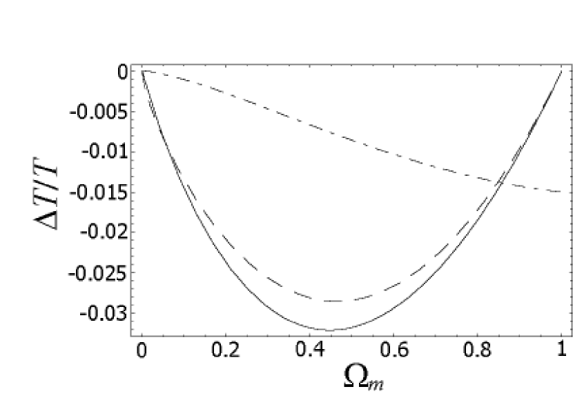
Figure 1: Amplitude of temperature anisotropy for a compensating void with $\delta_{m}=-0.3$ as a function of the mass density $\Omega_{m}$ with the contribution from the term proportional to $\delta_{m}$ in equation (46) (solid curve), in equation (B6) (dashed curve) and that from the term proportional to $\delta_{m}^{2}$ in equation (46) (dash-dotted curve). We assume $\xi_{2}\equiv r_{v2}R_{2}/H_{2}^{-1}=1$ and $\psi_{2}=0$.

For a void at $z=0$ in the flat-$\Lambda$ FRW universe with $\Omega_{m,0}=0.24$, (Spergel et al. 2006) we have $w_{0}=\Omega_{m,0}-1=-0.76$. Then equations (46) and (47) yield

$$\frac{\Delta T}{T} \approx \xi_{0}^{3}\cos{\psi_{2}}\biggl{[}0.087(\cos^{2}{\psi_{2}})\delta_{m,0}$$ (49)

$$- \bigl{(}0.021+0.018\cos^{2}{\psi_{2}}\bigr{)}\delta_{m,0}^{2}\biggr{]},$$

where $\xi_{0}$ and $\delta_{m,0}$ are evaluated at $t=t_{0}$. Plugging $\psi_{2}=0$ $(\theta=0)$ in equation (46), we have the anisotropy

$$\frac{\Delta T}{T}\approx(0.087\delta_{m,0}-0.039\delta_{m,0}^{2})\xi_{0}^{3}$$ (50)

toward the center of the void. From equation (50), we conclude that the contribution from the second-order effect, which is proportional to $\delta_{m}^{2}$ coherently enhances the contribution from the linear ISW effect provided that the second-order correction for the void expansion and the wall expansion (which we discuss later) is negligible. In this case, we would observe a cold spot in the direction of the void.

To generate an anisotropy $\Delta T/T=10^{-5}$, the void radius should be

$$r_{v}(z=0)\approx 2\times 10^{2}(|\delta_{m,0}|/0.2)^{-1/3}~{}~{}h^{-1}\textrm{Mpc},$$ (51)

where $H^{-1}_{0}=3000~{}h^{-1}$Mpc. In comparison with the equivalent void model in the EdS background, the void radius can be smaller because of the coherent contribution owing to the linear ISW effect and the second-order effect.

In order to study the second-order corrections, we introduce two nonlinear parameters ($\epsilon,\eta$) that control the void and the wall expansion (see also Inoue & Silk 2006). These are defined as

$$\delta_{H}=\frac{1+f^{-1}(w)}{2}\Omega_{m}\delta_{m}-\epsilon\delta_{m}^{2},$$ (52)

and

$$\beta=-\frac{\Omega_{m}^{0.6}}{6}\delta_{m}+\eta\delta_{m}^{2}.$$ (53)

If the matter inside the void near the boundary expands with the asymptotic velocity of the wall, i.e., $\delta_{H}=\beta$, then the non-linear parameter $\epsilon$ can be written as

$$\epsilon=\frac{1}{6\delta}\biggl{(}\Omega_{m}^{3/5}+3\Omega_{m}-6\delta\eta-5F^{-1}\Omega_{m}^{2/3}\biggr{)}.$$ (54)

Assuming $\eta=0$, we have $\epsilon>0$ for $\Omega_{m}>0$. For low-density universes $\Omega_{m}=0.2-0.3$, we have $\epsilon=(0.07-0.09)|\delta|^{-1}$. As shown in figure 2, an increase in $\epsilon$ leads to further redshifts of the photons due to reduction in the expansion rate inside the void. Therefore, for voids that expand with the asymptotic velocity, the second-order effect always enhances the linear ISW effect. On the contrary, for $\epsilon<0$, the second-order effect leads to further blueshifts of the photons. Therefore, for voids that expand sufficiently faster than the asymptotic velocity of the wall (i.e. $\delta_{H}>\beta$), the second-order effect can reduce the redshift of photons due to the linear ISW effect. Furthermore, an increase in the velocity of the wall (i.e. $\eta>0$) also leads to a suppression of the linear ISW effect because the photon is more Doppler blueshifted (see figure 2, right). Thus, the net redshift/blueshift of photons upon leaving the void depends on whether it is asymptotically evolving or not. In what follows, we define asymptotic voids as those with $\delta_{H}=\beta$ and $\eta=0$.

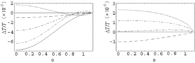
Figure 2: Second-order effects. Temperature anisotropy profiles owing to the second-order effect are plotted as a function of the subtending angle $\theta$. We assume a compensating void with a radius $r_{v}=200h^{-1}$ Mpc, $\delta_{m}=-0.3$, and the size/distance parameter $b=0.9$. Left:($\epsilon,\eta$)=(-0.3,0) (dotted curve), ($0,0$) (dashed curve), ($0.3,0$) (dash-dotted curve), and ($0.6,0$) (dash-dotted-dotted curve). Right:($\epsilon,\eta$)=($0,0.9$) (dotted curve), ($0,0.6$) (dash-dot-dotted curve), ($0,0.3$) (dash-dotted curve), and ($0,0$) (dashed curve). The solid curve in the left panel denotes the temperature anisotropy profile owing to the linear ISW effect.

3 Origin of anomalies

In order to explain the low-$l$ anomalies, we have proposed a model that consists of a pair of identical local voids in the direction $(l,b)=(-30^{\circ},-30^{\circ})$ at $z\sim 0.05$ (Inoue & Silk 2006). In the flat-$\Lambda$ background, a similar model can work as well. For illustrative purpose, we have simulated skymaps for models that consist of identical asymptotic voids with a density contrast $\sim-0.3$ that are tangent to each other. Note that we are assumed to be just outside one of the voids. As the background cosmology, we have assumed a flat-$\Lambda$ FRW model with $\Omega_{m,0}=0.24$. As shown in figure 3, the planar feature $l=2,3,6$ and the alignment feature $l=2,3$ can be well reproduced in our model that consists of identical voids with radius $(2-3)\times 10^{2}h^{-1}$ Mpc.

Although we still need an additional contribution that does not completely blur the fluctuation pattern by the voids, the chance of alignment between the quadrupole and octopole becomes large in our void model since otherwise no correlation between the two modes is expected.

In order to study the large-angle correlation feature, we also calculated the two-point correlation function in real space $C(\theta)$ (figure 4). For $r_{v}=300h^{-1}$ Mpc, the amplitude for the separation angle $\theta>30^{\circ}$ is found to be $C(\theta)\sim 100\mu\textrm{K}^{2}$ which is marginally consistent with the observed WMAP 3-year values (see Spergel et al. 2006).

Recently, it has been argued that the Shapley supercluster could be responsible for the anomalies on large angular scales (Cooray & Seto 2005; Rakić et al. 2006). However, as shown in figure 3, the amplitude in the direction to the Shapley supercluster (in the direction of the contact point of the two hypothesized voids) is somewhat smaller than those of the minima in either the quadrupole or the octopole. Furthermore, in the flat-$\Lambda$ FRW model, the presence of the linear ISW effect (blueshift effect for mass concentration) can reduce the amplitude of the temperature fluctuations due to the Rees-Sciama effect (redshift effect for mass concentration) in the quasi-linear regime (locally $\Omega_{m}\sim 1$). Because the highly non-linear structure ($\delta\gg 1$) is concentrated in a particular region, it cannot strongly affect the large angular fluctuations. Thus, we conclude that such a scenario has a potential difficulty in explaining the anomalies in the FRW model with a cosmological constant.

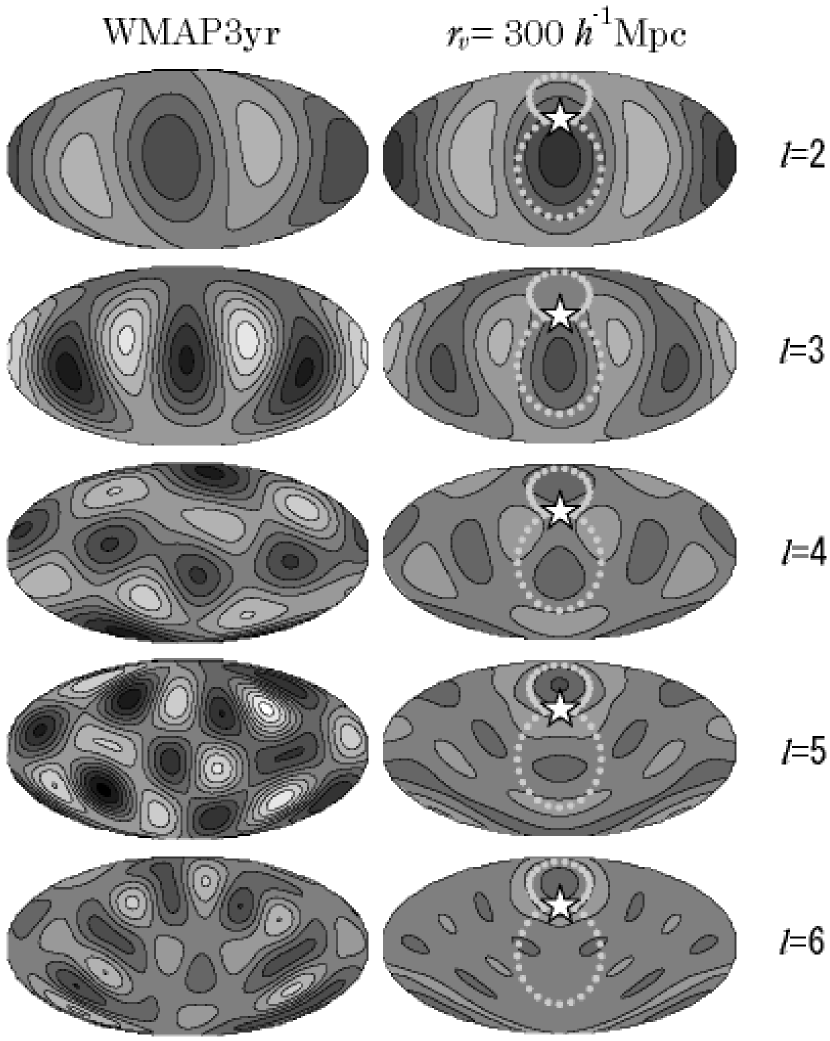
Figure 3: Mollweide projection maps for the cleaned CMB from the WMAP third-year data (Park et al. 2006) (left) and those for the temperature anisotropy owing to a pair of identical voids with radius $r_{v}=300h^{-1}$ Mpc (right) for modes $l=2-6$. We assume a flat-$\Lambda$ FRW universe with $\Omega_{m,0}=0.24$. The boundaries of the void hemispheres are denoted by small light-gray disks. Note that the identical voids are tangential to each other and the apparently larger void is nearer to us. We also assume that we are outside the pair of voids. The size/distance ratios of the two voids are assumed to be $b=0.91$ and $b=0.46$. The separation angle of the void centers is $\theta_{s}=63^{o}$ and the non-linear parameters are chosen to be $(\epsilon,\eta)=(0.27,0)$, which correspond to an asymptotic void $(\delta_{H}=\beta$). The gray scale denotes the temperature fluctuations in which the maximum absolute value is set to $50\mu$K. The north pole is aligned to the $z-$axis for which the angular dispersion of the quadrupole plus the octopole around the $z-$axis (de-Oliveira Costa et al. 2004) is maximal in the direction $(l,b)=(-110^{\circ},60^{\circ})$, which is close to the dipole direction at $(l,b)=(-96^{\circ},48^{\circ})$. The coordinate center is located at $(l,b)=(-30^{\circ},-30^{\circ})$. The Shapley supercluster is located in the direction of the point where the two voids contact each other (star).

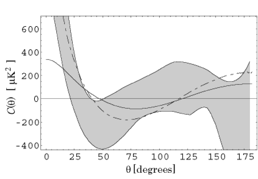
Figure 4: Two-point correlation function $C(\theta)$ for the void model as in figure 3 (solid curve) and for the WMAP three year data (gray region) expected for a statistically isotropic sky with best-fit $\Lambda$CDM cosmology and for the best-fit flat $\Lambda$CDM model with $\Omega_{b,0}=0.04$ and $\Omega_{m,0}=0.24$ (dash-dotted curve). The gray region denotes the maximum likelihood error at the 68% confidence level, which consists of the cosmic variance and the measurement errors.

4 Mean contribution from dust-filled voids

As shown in section 3, for linear voids $|\delta_{m}|\ll 1$ at $z<1$, the temperature anisotropy due to a dust-filled void in the flat-$\Lambda$ FRW background is proportional to $\delta_{m}r_{v}^{3}$ due to the linear ISW effect. Assuming the cold dark matter (CDM) power spectrum, the mean amplitude of the temperature anisotropy due to a linear void is proportional to $r_{v}$ because $|\delta_{m}|_{r.m.s}\propto r_{v}^{-2}$ for the linear regime. Therefore, we expect larger contributions from larger voids provided that $|\delta_{m}|_{r.m.s}\ll 1$ (solid curve in the right panel in figure 4). For quasi-linear voids $|\delta_{m}|_{r.m.s}=O(10^{-1})$, or linear voids at high $z$, the second-order effect can also contribute to the anisotropy. Because we have $|\delta_{m}|_{r.m.s}\propto r_{v}^{-1/3}$ for the non-linear regime, the contribution from the second-order effect is maximum at the scale $r_{v}\sim 2\times 10^{2}h^{-1}$ Mpc (dashed curve in the right panel in figure 5). In the high redshift region $z>1$, the contribution from the linear ISW effect is significantly reduced because the gravitational potential decay does not occur in the matter-dominant epoch. Similarly, the contribution from the second-order effect is also significantly reduced at $z>1$ (5, right).

From these features, we conclude that local dust-filled quasi-linear voids with a radius $r_{v}\sim 200h^{-1}$ Mpc are natural candidates for explaining the origin of the claimed anomalies on large angular scales.

However, one may argue that the possibility of having such large voids is extremely small. Indeed, if we assume a flat-$\Lambda$ CDM cosmology, we find that a $\sim 30\%$ mass deficiency at the scale of $r_{v}=200h^{-1}$ Mpc is only a $13\sigma$ result for linear fluctuations with $\sigma_{8}=0.74$ or $11\sigma$ for the preWMAP3 normalization $\sigma_{8}=0.9$. Assuming the CDM power spectrum (Bardeen et al. 1986), the expected temperature anisotropy for a linear (not asymptotic) void with radius $r_{v}=200h^{-1}$ Mpc at $z\sim 0$ is $\Delta T/T=O(10^{-7})$.

This inconsistency may be circumvented by considering a percolation process of small non-linear voids (Colombi et al. 2000; Hanami 2001). As $N-$body simulations (Colberg et al. 2005) and local observations (Patiri et al. 2006) suggest, at low redshifts $z<1$, non-linear voids with a typical radius of the order of $O(10)h^{-1}$ Mpc cover almost the entire space. Therefore, small non-linear voids can percolate each other to make larger dust-filled local quasi-linear voids. Interestingly, a low-density region with a $25\%$ deficiency at $z<0.1$ over a volume of $300h^{-1}\textrm{Mpc}^{3}$ has been discovered in the galaxy distribution in the south Galactic cap (Frith et al. 2003, 2005; Busswell et al. 2004). It seems that the underdense region consists of two local voids in the ranges $0.03<z<0.06$ and $0.07<z<0.1$, suggesting that the region consists of several dust-filled voids with a radius $r_{v}\sim 50h^{-1}$ Mpc.

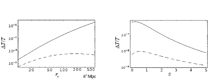
Figure 5: Mean amplitudes of temperature anisotropy for a linear void $|\delta_{m}|\ll 0.1$ as a function of void radius $r_{v}$ at $z=0$ (left),and as a function of void redshift $z$ for $r_{v}=200h^{-1}$ Mpc (right). Contribution from the linear ISW effect is denoted by solid curves and that from the second-order effect is denoted by dashed curves. We assume $(\epsilon,\xi)=(0.0)$ and cosmological parameters $(\Omega_{m,0},\Omega_{b,0},h,\sigma_{8},n)=(0.24,0.04,0.73,0.74,1)$ (Spergel et al. 2007).

If such a low-density region can be regarded as a homogeneous dust-filled asymptotically evolving void, we expect an anisotropy in the local Hubble constant $\delta_{H}\sim-\Omega_{m}^{0.6}\delta_{m}/6\sim 0.02$. It can be even larger than $\delta_{H}=(1+f^{-1}(w))\Omega_{m}\delta_{m}/2\sim 0.04$ if it is not asymptotically evolved. Although the substructure inside the void can also affect the anisotropy in the Hubble constant, we expect that the mean value over the low-density region will show a systematic deviation in comparison with the global value by several percent. Detection of a correlation between local large-scale structure and the anisotropy in the local Hubble constant would be strong evidence for the postulated local dust-filled large voids.

5 Summary and discussion

In this paper, we have explored the large angular scale temperature anisotropy owing to the homogeneous local dust-filled voids in the flat-$\Lambda$ FRW universe. A compensated asymptotically evolving dust-filled void with a comoving radius $r_{v}=(2-3)\times 10^{2}h^{-1}$ Mpc and a density contrast $\delta_{m}=-0.3$ will give a cold spot with anisotropy $\Delta T/T\sim-10^{-5}$. A pair of such compensated local voids in the direction $(l,b)=(-30^{\circ},-30^{\circ})$ might explain the quadrupole/octopole alignment and the planarity of quadrupole and octopole. As in the void model in the EdS background, the temperature anisotropy due to the dust-filled homogeneous void is proportional to $(r_{v}/H^{-1})^{3}$. For asymptotically evolving voids, contributions from the term that is proportional to $\delta_{m}^{2}$ always enhance the linear ISW effect which is proportional to $\delta_{m}$. However, for local voids that expand sufficiently faster than the asymptotic velocity of the wall, contributions from the term $\propto\delta_{m}^{2}$ can suppress the linear ISW effect. Thus the enhancement/suppression depends on the non-linear dynamics of the void. We have also shown that the contribution to the CMB anisotropy from the linear ISW and the second order effects is more significant for local voids at $z<1$ than those at high redshifts $z>1$.

Assuming the CDM power spectrum based on the standard inflationary scenario, the expected amplitude of the temperature anisotropy owing to the linear void with radius $r_{v}=2\times 10^{2}h^{-1}$ Mpc is just $\Delta T/T=O(10^{-7})$. However, at low redshifts $z<1$, percolation of small non-linear voids could make large quasi-linear voids with a density contrast $|\delta_{m}|\sim 0.1$. The observed low-density region with a $25\%$ deficiency at $z<0.1$ over a volume of $300h^{-1}\textrm{Mpc}^{3}$ in the south Galactic cap (Busswell et al. 2004) might be evidence of such a structure. Detailed observational properties can be obtained by ongoing projects such as the 6dF galaxy survey (Heath et al. 2004). On the theoretical side, more elaborate modeling of the void percolation process is required because the signature on the CMB may depend on the configuration and the momentum of the substructure inside the void. Determination of non-linear parameters $(\epsilon,\eta)$ based on more realistic models is also an important task. Once these observational and theoretical issues are settled, we can determine whether new physics, such as primordial non-Gaussianity (Mathis et al. 2004) or an enhancement in the gravity in the dark energy sector (Farrar & Rosen 2006), may be required.

Another implication unique to the dust-filled large voids postulated here concern increased dispersion in the locally measured Hubble constant as measured both in different directions and at different redshifts. As we have shown, for voids with a density contrast $\delta_{m}=-0.3$, the expected fluctuation in the Hubble constant is as large as $2-4\%$ (Tomita 2000, 2001). Although, in this paper, we have assumed that we are outside the dust-filled voids, it is also possible that we are inside the void. If the distance between the Milky Way and the wall of the void is sufficiently small, the ratio of our peculiar velocity to the light velocity will be $v/c=O(10^{-3})$ for a radius $r_{v}=(2-3)\times 10^{2}h^{-1}$ Mpc, and a density contrast $\delta_{m}=-0.3$. Therefore, the order of the predicted amplitude of the dipole is similar to that of the observed CMB dipole (Tomita 2003). In this case, we expect a positively skewed dispersion in the Hubble constant $\delta_{H}\sim 0.02-0.04$ in the direction to the center of the void (approximately at $(l,b)=(-30^{\circ},-30^{\circ})$). Accuracy measurement of $\sim 1\%$ in the Hubble constant would be achieved by increasing the number of samples of Type Ia supernovae from $N\sim 50$ to $5000$ provided that the error decreases as $1/\sqrt{N}$.

Another approach to peculiar velocities uses galaxy surveys that apply different distance calibrators (Pike & Hudson 2005; Watkins and Feldman 2007). The most optimistic individual galaxy distance estimates cited, using $I$-band surface brightness fluctuations, have an accuracy of 10% for half the sampled galaxies and extend to 40$h^{-1}$Mpc (Tonry et al. 2001). Other studies go deeper, for example the Tully-Fisher relation has been applied to a sample of 3000 spiral galaxies out to 200$h^{-1}$Mpc (Karachentsev et al. 2006) with distance errors of 15%. It should be possible to apply these techniques to test our hypothesis by targeting several thousand galaxies that sample the peculiar velocities induced by our nearest postulated voids and their associated shells, which extend over thousands of square degrees.

Thus further study of correlation between the large scale structure and the variation in the locally measured Hubble constant is necessary in order to prove/disprove our void scenario.

Our findings may shed new light on the issue of cross-correlation between the large-scale structure and the CMB. Within a flat $\Lambda$CDM model, recent works on the cross-correlation suggest a best-fit value $\Omega_{\Lambda}\sim 0.85$ (Rassat et al. 2006; Cabre et al. 2006), which is larger than the best-fit value $\Omega_{\Lambda}=0.70$ from the joint analysis of the CMB and the large-scale structure (Tegmark et al. 2004). Because the second order effect in quasi-linear asymptotic voids systematically enhances the linear ISW effect, the observed deviation could be explained by such quasi-linear or non-linear local voids in the flat-$\Lambda$ universe with $\Omega_{\Lambda}=0.70$.

If the low$-\ell$ CMB anomalies persist, our phenomenological model provides a simple astrophysical interpretation with no recourse to new physics. Perhaps the most promising tests of our hypothesis will come from improved sampling of Hubble flow anisotropies. If these directions coincide with the locations of our postulated voids, the case becomes more compelling. CMB polarisation maps and lensing studies could potentially reveal interesting signals. For example, the inflow pattern in the void wall will induce a small polarisation signal, as will the associated gravitational lensing of the CMB. The expected amplitude of the scattering angle of photons due to the postulated large local voids is $\sim\delta_{m}^{2}\xi^{2}\sim 0.1^{\circ}$, corresponding to subdegree scales. These effects are small, amounting to an imprint on the ambient polarisation pattern of order a percent ($\sim v/c$), but the phase structure would be unique and correlated with both the temperature map and the large-scale galaxy distribution. The global mean value of the Hubble constant will be slightly reduced, as the required dominance of voids biases the measured local $H_{0}$ to be slightly high. Although the effect is small, it has potential significance for future dark energy surveys, which will combine CMB studies with deep galaxy redshift surveys. For example, the degeneracy between the Hubble constant and the determination of the curvature of the universe using the CMB will need to be taken into account.

One anomaly we have not sought to incorporate explicitly is the north-south power excess in the CMB. It may be tempting to attribute this to a directional deficiency of local power, as has been previously noted in deep galaxy counts (Busswell et al. 2004) and which in the present context consists of a compensated void complex that correlates the CMB and large-scale structure signals.

The reduction in normalisation of $\sigma_{8}$ to 0.74 makes it more difficult to account for large-scale features in the galaxy distribution without introducing extra large-scale power. Our example of tuned voids is one manifestation of extra power that would inevitably, if incorporated into the cosmological initial conditions of a simulation, boost the significance of large-scale features such as the SDSS “Great Wall” (Gott et al. 2005) and rare massive clusters (Baugh et al. 2004).

Appendix A Linear perturbation of Hubble parameter

In what follows, we calculate the Hubble parameter contrast at the matter- or $\Lambda$-dominant era in the linear order. Let us write the Friedmann equation at a point ${\mathbf{x}}$ in a perturbed universe in terms of the scale factor $a$, the Hubble parameter $H$, the matter density $\rho_{m}$, the gravitational constant $G$, the curvature $K$, and the cosmological constant $\Lambda$ as

$$H^{2}({\mathbf{x}},t)=\frac{8\pi G}{3}\rho_{m}({\mathbf{x}},t)-\frac{K({\mathbf{x}},t)}{a^{2}(t)}+\frac{\Lambda}{3}$$ (A1)

where the Hubble parameter $H$ is defined on a comoving slice and the scale factor at the present time $t_{0}$ is assumed to be $a_{0}=1$. In what follows, we introduce the total density $\rho=\rho_{m}+\frac{\Lambda}{8\pi G}$. The linear perturbation component in equation (A1) in the Fourier space for the flat FRW background can be written as

$$2\bar{H}\delta H_{\mathbf{k}}=\frac{8\pi G}{3}\delta\rho_{\mathbf{k}}-\frac{2}{3}\biggl{(}\frac{k}{a}\biggr{)}^{2}{\cal{R}}_{\mathbf{k}},$$ (A2)

where $\bar{H}$ is the spatially averaged Hubble parameter and the curvature perturbation ${\cal{R}}$ is defined as

$$\delta K_{\mathbf{k}}=\frac{2}{3}k^{2}{\cal{R}}_{\mathbf{k}}.$$ (A3)

If we can neglect the anisotropic stress, the relation between the Newtonian gravitational potential $\Phi_{\mathbf{k}}$ and the total energy density contrast $\delta_{\mathbf{k}}$ is given by the Poisson equation

$$-\biggl{(}\frac{k}{a}\biggr{)}^{2}\Phi_{\mathbf{k}}=4\pi G\delta\rho_{\mathbf{k}}.$$ (A4)

The time evolution of $\delta$ is given by the continuity equation

$$\dot{\delta\rho}_{\mathbf{k}}=-3(\bar{\rho}+\bar{P})\delta H_{\mathbf{k}}-3\bar{H}\delta\rho_{\mathbf{k}},$$ (A5)

where $\bar{\rho}$ and $=\bar{P}$ are the spatially averaged total energy density and total pressure, respectively. The perturbed Raychaudhuri equation is (Liddle & Lyth 2000)

$$\dot{\delta H}_{\mathbf{k}}=-2\bar{H}\delta H_{\mathbf{k}}-\frac{4\pi G}{3}\delta\rho_{\mathbf{k}}+\frac{1}{3}\biggl{(}\frac{k}{a}\biggr{)}^{2}\frac{\delta P_{\mathbf{k}}}{\bar{\rho}+\bar{P}}.$$ (A6)

From equations (A2-A6), we have

$$\frac{2}{3}\bar{H}^{-1}\dot{\Phi}_{\mathbf{k}}+\frac{5+3w}{3}\Phi_{\mathbf{k}}=-(1+w){\cal{R}_{\mathbf{k}}},$$ (A7)

where the effective equation of state $w=\bar{P}/\bar{\rho}$ is written in terms of the density parameter for the matter $\Omega_{m,0}$ and that for the cosmological constant $\Omega_{\Lambda,0}$ at the present time $t_{0}$ as

$$w=-\frac{1}{\Omega_{m,0}/(\Omega_{\Lambda,0}~{}a^{3})+1}.$$ (A8)

From the time derivative of the local Friedmann equation (A2) multiplied by $a^{2}$, the continuity equation (A5), and the Raychaudhuri equation (A6), we have ${\dot{\cal{R}}_{\mathbf{k}}}=-\bar{H}\delta P_{\mathbf{k}}/(\bar{\rho}+\bar{P})=0$ because the pressure perturbation vanishes $\delta P_{\mathbf{k}}=0$ at the matter- or $\Lambda$- dominant era. Plugging $\Phi_{\mathbf{k}}=f(w){\cal{R}_{\mathbf{k}}}$ into equation (A7), since ${\dot{\cal{R}}_{\mathbf{k}}}=0$, $f(w)$ satisfies

$$2w(1+w)\frac{df}{dw}+\frac{5+3w}{3}f+1+w=0.$$ (A9)

The solution is

$$f(w)=-\frac{3}{5}(1+w)^{1/3}{}_{2}F_{1}\biggl{[}\frac{5}{6},\frac{1}{3},\frac{11}{6},-w\biggr{]},$$ (A10)

which satisfies the boundary condition $f=-3/5$ for $w=0$. Plugging $\Phi_{\mathbf{k}}=f(w){\cal{R}_{\mathbf{k}}}$ into equation (A2) and (A4), we have

$$\frac{\delta H_{\mathbf{k}}}{\bar{H}}=\frac{1+f^{-1}(w)}{2}\delta_{\mathbf{k}},$$ (A11)

which yields

$$\delta_{H}=\frac{1+f^{-1}(w)}{2}\delta_{m}\Omega_{m},$$ (A12)

where the evolution of $f(w)$ is given by equation(A8) and (A10). The equation (A12) is applicable to the matter- or $\Lambda$- dominated era at which the anisotropic stress is negligible.

Appendix B Linear integrated Sachs-Wolfe effect

We evaluate the magnitude of the linear integrated Sachs-Wolfe (ISW) effect, which comes from the time evolution of the gravitational potential as the photon traverses the void.

In terms of the gravitational potential $\Psi$ , contribution from the ISW effect is approximately evaluated as

$$\frac{\Delta T}{T}\sim\frac{\partial\Psi}{\partial t}\Delta t,$$ (B1)

where $\Delta t$ is the duration time for which the photons pass through the void. From the Poisson equation, in the Newtonian limit, $\Delta t\ll H_{0}^{-1}$, the gravitational potential can be written in terms of the density contrast $\delta_{\mathbf{k}}=\delta\rho_{\mathbf{k}}/\rho$ inside the void in the Fourier space as

$$\dot{\Psi}_{\mathbf{k}} \sim -\frac{1}{k^{2}}\frac{\partial}{\partial t}(H^{2}a^{2}\delta_{\mathbf{k}})$$ (B2)

$$= -\frac{1}{k^{2}}(2\dot{a}\ddot{a}\delta_{\mathbf{k}}+\dot{a}^{2}\dot{\delta}_{\mathbf{k}})$$

where a dot means the partial time derivative $\cdot\equiv\frac{\partial}{\partial t}$ and $k$ is the wavenumber. Plugging the peculiar velocity inside the void at comoving distance $r$ from the center $v=\delta_{H}Har$ into the continuity equation

$$\frac{\partial\delta}{\partial t}+a^{-1}\nabla\cdot\mathbb{v}=0,$$ (B3)

we have

$$\dot{a}^{2}\delta_{\mathbf{k}}^{2}=-3H^{3}a^{2}\alpha\delta_{\mathbf{k}},$$ (B4)

where $\alpha=(1+f^{-1}(w))/2$. Writing the wavenumber in terms of the void comoving radius $r_{v}$ as $k\sim\pi/r_{v}$, equation (B2) and equation (B4) yield,

$$\frac{\Delta T}{T}\sim-\frac{1}{\pi^{2}}\xi^{3}(2q+3\alpha)\delta,$$ (B5)

where $\xi=ar_{v}/H^{-1}$ and $q$ is the deceleration parameter. Thus, the anisotropy owing to the linear ISW effect is proportional to the density contrast $\delta$ and $\xi^{3}$. In terms of the matter density contrast $\delta_{m}=\delta\rho_{m}/\rho_{m}$ and the matter density parameter $\Omega_{m}$, equation (B5) can be written as

$$\frac{\Delta T}{T}\sim s\xi^{3}\delta_{m}\Omega_{m},$$ (B6)

where

$$s=-\frac{1}{\pi^{2}}\biggl{(}3\Omega_{m}-\frac{1}{2}-\frac{5}{2}\Omega_{m}^{-1/3}F^{-1}\biggr{)}.$$ (B7)

References

- (1)
- (2) Arnau, J.V., Fullana, M.J., Monreal, L. & Sáez, D. 1993, ApJ, 402, 359
- (3) Bardeen, J.M., Bond J.R., Kaiser N, & Szalay A.S. 1986, ApJ, 304, 15
- (4) Baugh, C. et al. 2004 MNRAS, 351, L44
- (5) Busswell, G.S., Shanks, T., Outram, P.J.,Frith, W.J., Metcalfe N., & Fong R. 2004 MNRAS, 354, 991
- (6) Cabre, A., Gaztanaga, E., Manera, M., Fosalba, P., & Castander F. 2006, MNRAS, 372, L23
- (7) Chiang, L.-Y., Naselsky, P., & Coles, P. 2004, ApJ, 602, L1
- (8) Colberg, J.M., Sheth, R.K., Diaferio, A., Liang G.,M. & N. Yoshida, 2005 MNRAS, 360, 216
- (9) Colombi, S., Pogosyan, D., & Souradeep, T. 2000, PRL, 85, 5515
- (10) Cooray,. A. & Seto, N. 2005, JCAP, 0512, 004
- (11) Copi, C.J., Huterer, D., Starkman, G.D. 2004, PRD, 70, 043515
- (12) Cruz, M., Martínez-González E., Vielva, P., & Cayon, L. 2005 MNRAS, 356, 29
- (13) de Oliveira-Costa, A., Tegmark, M., Zaldarriaga, M.,& Hamilton, A. 2004, PRD 69, 063516
- (14) Eriksen, H.K., Hansen, F.K., Banday, A.J., Goŕski, K.M., & Lilje, P.B. 2004, ApJ, 605, 14
- (15) Farrar, G.R. & Rosen R.A. 2007, PRL, in press(astro-ph/0610298)
- (16) Frith, W.J., Busswell, G.S., Fong, R., Metcalfe N., & Shanks, T. 2003 MNRAS 345, 1049
- (17) Frith, W.J., Shanks, T., & Outram, P.J. 2005 MNRAS 361, 701
- (18) Fullana, M.J., Arnau, J.V., & D. Sáez 1996 MNRAS, 280, 1181
- (19) Gott, R. et al. 2005, ApJ, 624, 463
- (20) Griffiths, L., Kunz, M., & Silk, J. 2003, MNRAS, 339, 680
- (21) Hanami, H. 2001, MNRAS, 327, 721
- (22) Hansen, F.K., Balbi, A., Banday, A.J., & Goŕski, K.M. 2004 MNRAS, 354, 905
- (23) Inoue, K.T. & J.Silk 2006, ApJ, 648, 23
- (24) Jaffe, T.R., Banday A.J., Eriksen, H.K., Goŕski, K.M., & Hansen F.K. 2005 ApJ629, L1
- (25) Jones, D. H., et al., 2004 MNRAS, 355, 747
- (26) Karachentsev, I. et al. 2006, Astrofizika, 49, 527
- (27) Larson, D.L. & Wandelt, B.D. 2004 ApJ613, L85
- (28) Liddle, R.L. & Lyth D.H. 2000 Cosmological Inflation and Large-Scale Structure (Cambridge:Cambridge Press), 99
- (29) Luminet, J.-P., Weeks, J.R., Riazuelo, A.,Lehoucq, R., & Uzan, J.-P. 2003, Nature, 425, 593
- (30) Martínez-González, E., Sanz, J.L., & Silk J. 1990, ApJ, 355, L5
- (31) Mathis, H. et al. 2004, MNRAS, 350, 287
- (32) Mészáros, A. & Molnár Z. 1996 ApJ, 470, 49
- (33) Moffat, J.W. 2005, JCAP, 10, 012
- (34) Panek, M. 1992, ApJ, 388, 225
- (35) Park, C. 2004, MNRAS, 349, 313
- (36) Park, C.-G., Park, C., & Gott III, R. J. 2006, preprint (astro-ph 0608129)
- (37) Patiri, S.G., Betancort-Rijo, J., Prada, F., Klypin, A., & Gottlöber, S. 2006, MNRAS, 369, 335
- (38) Pike, R.W. & Hudson, M. 2005, ApJ, 635, 11
- (39) Rakić A., Rasanan S, & Schwartz D.J. 2006, MNRAS, 369, L27
- (40) Rassat, A., Land, K., Lahav, O., & Abdalla, F.B., 2007, MNRAS, in press (astro-ph/0610911)
- (41) Rees, M. & Sciama D.W. 1968, Nature 217, 511
- (42) Sakai, N., PhD thesis, 1995, Waseda Univ.
- (43) Sakai, N., Sugiyama, N., & Yokoyama J. 1999 ApJ, 510, 1
- (44) Schwarz, D.J., Starkman, G.D., Huterer, D., & Copi, C.J 2004 PRL, 93, 221301
- (45) Spergel, D.N., et al. 2007, ApJ, in press (astro-ph/0603449)
- (46) Tegmark, M., de Oliveira-Costa, A., & Hamilton, A.J.S. 2003, PRD 68, 123523
- (47) Tegmark, M. et al. 2004, PRD, 69, 103501
- (48) Thompson, K.L. & Vishniac, E.T. 1987, ApJ, 313, 517
- (49) Tomita, K. 2000, ApJ, 529, 26
- (50) Tomita, K. 2001, Prog. Theo. Phys., 105, 419
- (51) Tomita, K. 2003, ApJ, 584, 580
- (52) Tomita, K. 2005a, PRD 72, 043526; 2006, PRD 73, (erratum 73, 029901[2006])
- (53) Tomita, K. 2005b, PRD 72, 103506
- (54) Tonry, J. et al. 2001, ApJ, 546, 681
- (55) Vadas, S. L. 1998, MNRAS, 299, 285
- (56) Vale, C. 2005, submitted (astro-ph/0509039)
- (57) Vielva, P., Martínez-González E., Barreiro, R.B., Sanz, J.L., & Cayon, L. 2004, ApJ, 609, 22
- (58) Watkins, R. & Feldman, H. 2007, preprint (astro-ph/0702751)