Photometric Redshifts of Galaxies in COSMOS¹

Abstract

We present photometric redshifts for the COSMOS survey derived from a new code, optimized to yield accurate and reliable redshifts and spectral types of galaxies down to faint magnitudes and redshifts out to $z\sim 1.2$. The technique uses $\chi^{2}$ template fitting, combined with luminosity function priors and with the option to estimate the internal extinction (or $E(B-V)$). The median most-probable redshift, best-fit spectral type and reddening, absolute magnitude and stellar mass are derived in addition to the full redshift probability distributions. Using simulations with sampling and noise similar to those in COSMOS, the accuracy and reliability is estimated for the photometric redshifts as a function of the magnitude limits of the sample, S/N ratios and the number of bands used. We find from the simulations that the ratio of derived 95% confidence interval in the $\chi^{2}$ probability distribution to the estimated photometric redshift ($D_{95}$) can be used to identify and exclude the catastrophic failures in the photometric redshift estimates.

To evaluate the reliability of the photometric redshifts, we compare the derived redshifts with high-reliability spectroscopic redshifts for a sample of 868 normal galaxies with $z<1.2$ from $z$COSMOS. Considering different scenarios, depending on using prior, no prior and/or extinction, we compare the photometric and spectroscopic redshifts for this sample. The rms scatter between the estimated photometric redshifts and known spectroscopic redshifts is $\sigma(\Delta(z))=0.031$, where $\Delta(z)=(z_{phot}-z_{spec})/(1+z_{spec})$ with a small fraction of outliers ($<2.5\%$)- (outliers are defined as objects with $\Delta(z)>3\sigma(\Delta(z))$ where $\sigma(\Delta(z))$ is the rms scatter in $\Delta(z)$). We also find good agreement ($\sigma(\Delta(z))=0.10$) between photometric and spectroscopic redshifts for Type II AGNs.

We compare results from our photometric redshift procedure with three other independent codes and find them in excellent agreement. We show preliminary results, based on photometric redshifts for the entire COSMOS sample (to $i<25$ mag.).

1 INTRODUCTION

The determination of galaxy redshifts is a prerequisite to studies of their cosmological evolution- measuring both distance-dependent quantities such as luminosities, masses and star formation rates and in specifying the lookback times. Redshifts are also necessary to separate out large scale structures and galaxies along the line of sight. With the advent of new sensitive detectors on large ground-based telescopes (Subaru, VLT, Keck) and space-borne facilities (HST, Spitzer, GALEX), we have now been able to perform extensive galaxy surveys to unprecedented depths. Measurement of spectroscopic redshifts to these galaxies is limited by two factors: their faintness (Papovich et al.  2006; Mobasher et al.  2005; Yan et al.  2005) and the large number of galaxies for which such information is needed (Wolf et al.  2004; Mobasher et al.  2004; Ilbert et al.  . 2006; Salvato et al.  2006).

Recently, photometric redshifts have been used extensively in deep cosmological surveys, yielding the galaxy luminosity functions (Dahlen et al.  2005; Caputi et al.  2005) and the evolution of star formation rates (Gabasch et al.  2004; Giavalisco et al.  2004; Dahlen et al.  2006). The photometric redshift technique has the advantage of providing redshifts for large samples of faint galaxies with a relatively modest investment in observing time. For maximal success with photometric redshifts the photometry should cover as wide a range in wavelength as possible. The principle disadvantage of the photometric redshifts is the relatively low resolution in wavelength and redshift (due to the width of filters) compared to spectroscopic redshifts. Photometric redshifts are, however, vital in resolving redshift ambiguities where spectroscopy shows only a single spectral line (Lilly et al.  2006).

In this paper we present measurements of photometric redshifts for galaxies in the Cosmic Evolution Survey (COSMOS) and explore the accuracy of the photometric redshifts based on extensive simulations, comparison with spectroscopic redshifts from zCOSMOS (Lilly et al.  2006) and with photometric redshifts estimated from a number of other independent algorithms. Over the $1.4^{\circ}\times 1.4^{\circ}$ area covered by COSMOS, we detect 367,000 galaxies to $i\sim 25$ (Capak et al.  2006), making it difficult to obtain spectroscopic redshifts for the entire galaxy sample. Extensive multi-waveband photometric data are now available for these galaxies, allowing measurement of photometric redshifts for a complete sample. These results are used to identify the large scale structures (Scoville et al.  2006; Finoguenov et al.  2006; Guzzo et al.  2006), to study the evolution of density-morphology relation (Capak et al.  2006), dependence of the star formation activity on the environment (Mobasher et al.  2006) and study of morphologies and rest-frame properties of individual galaxies (Scarlatta et al.  2006; Zamojski et al.  2006).

We present the photometric redshift technique in §2 followed by the photometric observations and photometric data in §3. In §4 we present simulations to explore the dependence of photometric redshifts to the magnitude limit, photometric accuracy and S/N ratios. We compare photometric and spectroscopic redshifts to a sample of galaxies with available such data in §5. In §6 we compare results from various photometric redshift codes. We summarise the galaxy properties derived from the photometric data, including SED types and stellar mass measurements in §7.

In this paper we use the standard cosmology with $\Omega_{M}=0.3$, $\Omega_{\Lambda}=0.7$, and $h=0.7$. Magnitudes are given in the AB-system unless otherwise stated.

2 Photometric Redshift Technique

The photometric redshift code developed for COSMOS is based on template fitting technique (Gwyn 1995; Mobasher et al.  1996; Chen et al.  1999; Arnouts et al.  ., 1999; Benitez 2001; Bolzonella et al.  2000; ). The templates, representing the rest-frame Spectral Energy Distribution (SED) for galaxies of different types, are convolved with the response functions of filters used in the COSMOS photometric observations. These were then shifted in redshift space and fitted to the observed SEDs of individual galaxies by minimizing the $\chi^{2}$ function,

$$\chi^{2}=\Sigma_{i=1}^{n}((F^{i}_{obs}-\alpha F^{i}_{template})/\sigma^{i})^{2}$$

The summation is over the passbands (i.e. number of photometric points) and $n$ is the total number of passbands. $F^{i}_{obs}$ and $F^{i}_{template}$ are, respectively, the observed and template fluxes for each passband; $\sigma^{i}$ is the uncertainty in the observed flux and $\alpha$ is the overall flux normalisation. The redshift corresponding to the centroid of redshift probability distribution and SED (i.e. spectral type) yielding the minimum $\chi^{2}$ value are then assigned to each galaxy. The redshift probability function for each galaxy is defined as $p(z,T)=e^{-\chi(z,T)^{2}/2}$, where $z$ and $T$ are respectively, the redshift and spectral type of galaxies. The estimated redshift corresponds to the centroid of this probability distribution, defined as

$$z=\frac{\int^{T_{max}}_{T_{min}}\int^{z_{max}}_{z_{min}}p(z,T)zdzdT}{\int^{T_{max}}_{T_{min}}\int^{z_{max}}_{z_{min}}p(z,T)dzdT}$$

This is used as the best estimate for the photometric redshifts in this study. The code gives the option of using Bayesian priors based on luminosity functions (LFs). The main effect of a LF prior is to discriminate between cases in which the redshift probability distribution shows multiple peaks due to ambiguity between the Lyman and 4000 Å  features. The inferred absolute magnitudes of the galaxy if it is at either of the redshift peaks can then be used to discriminate between these possibilities (i.e. an implied absolute magnitude significantly brighter than $M^{\ast}$ is increasingly unlikely). Thus, for each redshift, we calculate the rest-frame absolute V-band magnitude and compare it to the LF. For this study we use a Schecter LF with $M^{\ast}=-22$ mag and faint-end slope $\alpha=-1.26$. This corresponds to the mean of the characteristic magnitudes and faint-end slopes of the B-band luminosity functions for all spectral types of galaxies and over the redshift range $0<z<1$ (Dahlen et al. 2005), converted to V-band absolute magnitude using rest-frame $B-V$ colors. Compared to B-band, the V-band luminosity function (LF) is less sensitive to details of the spectral types of galaxies, allowing us to use a single LF for all types. In any case, the final photometric redshifts are not dependent on the LF used. Evolution with redshift of both $M_{V}^{\ast}$ and faint-end slope of the LF (Dahlen et al 2005) are incorporated into the LF prior. Nevertheless, we explored sensitivity of our results on different choices of $M^{\ast}$ and $\alpha$ and found them to be relatively insensitive to the choice of these parameters. Finally, using the spectroscopic sample (section 4.3), we optimised the prior LF parameters to minimise the scatter between the estimated photometric and spectroscopic redshifts.

We also include internal extinction ($E_{B-V}$) as a free parameter in the $\chi^{2}$ minimisation process (alongside redshift and spectral types) and estimate $E_{B-V}$ for individual galaxies using Galactic extinction law for early-type galaxies and Calzetti law (Calzetti et al.  2000) for late-type and starbursts. Absorption due to intergalactic HI is included using the parametrization in Madau (1995).

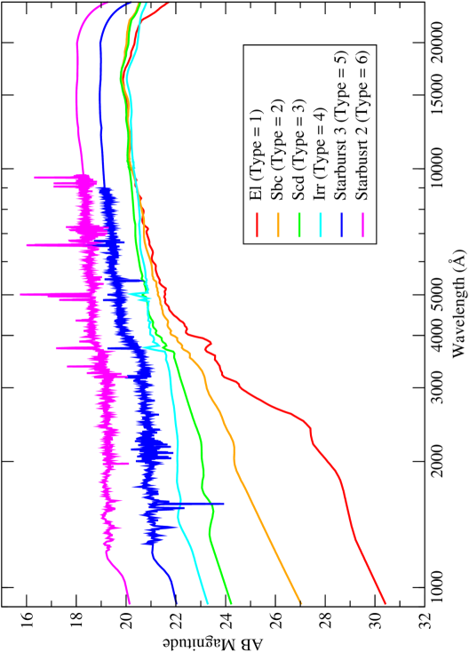
Figure 1: Spectral Energy Distributions used as templates for photometric redshift measurement. These are trained to minimise the residuals between the photometric and spectroscopic redshifts for a sample of galaxies in HDF-N with available such data.

Basic template spectral energy distributions (SEDs) for normal galaxies (E, Sbc, Scd and Im) from Colman et al.  (1980) and two starburst templates are from Kinney et al.  (1996)-(SB2 and SB3- Figure 1). The templates are corrected for systematic calibration errors and extended to the ultraviolet and infrared wavelengths using the method of Budavari et. al. (2000). The template corrections were derived from over 3000 galaxies with spectroscopic redshifts in the Hawaii Hubble Deep Field North (H-HDFN) (Capak et. al. 2004; Cowie et al.  2004; Wirth et al.  2004; Treu et al.  2005; Steidel et al.  2004; Erb et al.  2004). These galaxies had deep optical and infrared photometry (U,B_J,V_J,R_c,I_c,z⁺,J,H,K_s,HK^′)- (Capak et al. 2004; Bundy et al. 2005; Wang et al. 2005). Our corrections in the optical and UV are consistent with the calibration errors estimated by Coleman et al.  (1980) and Kinney et al.  (1996). The largest correction is in the UV where Coleman et al. (1980) forced agreement between their ground-based and IUE data. The infrared properties of our templates do differ significantly from those extended using Bruzual & Charlot (2000) models (Bolzonella et al.  2000). This is not surprising since stellar population models have large uncertainties in the infrared (Maraston 2005). The details of our template optimisation method will be discussed in Capak et al. (in prep 2007). The final, modified template SEDs are shown in Figure 1. we constructed intermediate-type templates from the weighted mean of the adjacent templates, defining five intermediate-type templates between the main spectral types. Our fitting therefore included a total of 31 SED templates, each redshifted between $z=0$ and $z=6$ in $\Delta z=0.01$ steps.

3 Photometric Data

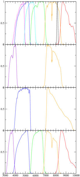
Figure 2: Total Response Functions for the filters used in photometric observations and photometric redshift measurement of the COSMOS. The filters consist of: top panel: B_jV${}_{j}g^{+}r^{+}i^{+}z^{+}$ and $NB816$ (Subaru/SupremeCam); second panel: u^∗ and $i^{*}$ (CFHT); Third panel: B_j and I_c; Forth panel: u’g’r’i’z’ (SDSS)

The photometric observations for COSMOS were carried out at optical ($u^{\ast}$: CFHT; BgVriz: SuprimeCam/Subaru; $i-$: CFHT; $i_{814}$: ACS/HST) and near-Infrared ($K_{s}$: Flamingos/CTIO and Kitt Peak) wavelengths. We also obtained narrow-band survey of the COSMOS field at 815 nm (NB815 filter) with SupremeCam/Subaru. The response functions for these filters are shown in Figure 2. Table 1 lists the filters, including the effective wavelength and band-width for each filter and the corresponding depth and image seeing. Details of the ground-based observations and data reduction are presented in Capak et al.  (2006) and Taniguchi et al. (2006).

The reduced images in all bands were PSF matched by Gaussian convolution with FWHM corresponding to the worst seeing (1.5” in $K_{s}$ band), allowing for non-Gaussian wings of the PSFs. The multi-waveband photometry catalog was then generated using SExtractor (Bertin & Arnout 1995). This is first done by measuring the total ($mag_{auto}$) and aperture (3” diameter) magnitudes on the detection image ($i-$band) and, for each galaxy, estimate the correction from aperture to total magnitudes. This correction is subsequently applied to the respective galaxies, detected in other bands. Details of the photometry, star/galaxy separation and catalog generation are given in Capak et al.  (2006).

In the next section we simulate the COSMOS catalog by constructing a similar mock galaxy catalog with the same filters, depths and SED shapes and assign a random redshift to each simulated galaxy. The simulated catalog will then be used to test the accuracy of our estimated photometric redshifts and the consistency of our technique. This will be further examined by comparing the photometric and spectroscopic redshifts to a sample of COSMOS galaxies with available such data.

4 Simulations

4.1 Mock Catalog

To explore the accuracy of photometric redshifts, we generated mock catalogs consisting of galaxies with the SEDs shown in Figure 1 and photometry measured in the same filters used for COSMOS (Figure 2). The aims of the simulation is to explore dependence of the photometric redshifts on the $S/N$ ratio, magnitude limit, redshift and galaxy type and how we could minimise the number of outliers (objects with very different output and input photometric redshifts).

We use the rest-frame B-band LFs derived for different spectral types of galaxies, using the GOODS data (Dahlen et al.  2005); therefore, both the type-dependence and evolution of the LFs are incorporated into the simulations. Each galaxy is assigned a random absolute magnitude in the range $-24<M_{B}<-16$ mag and spectral type, drawn from the type-dependent LFs. The six galaxy templates are the same as used in the photometric redshift calculation (§2). To each simulated galaxy, we also specified a redshift in the range $0<z<6$.

For any given galaxy, the K-correction in each band was estimated by convolution of the filter responses with the SED associated with that galaxy, shifted to its assigned redshift. We then estimate the apparent magnitudes using the rest-frame absolute magnitudes and the distance moduli. We restrict the mock catalog to galaxies with apparent magnitudes (in any given band) brighter than the observed magnitude limits in COSMOS (Table 1). We also assign photometric errors to each magnitude, depending on the S/N ratios with the same depth as real COSMOS data. Ideally, the photometric errors need to be estimated, also taking into account blending or defects on the images (sources near bright objects and internal camera reflections). This can be performed by distributing images of galaxies with known mag/type/redshift into the existing multi-band images, apply the same photometric measurement scheme and then running the photometric redshift code. Therefore, simulations here only provide an internal consistency check in reproducing the input parameters.

The resulting catalog consists of simulated data, including: magnitudes and their associated errors in the same filters as in the initial COSMOS catalog, redshifts and spectral types for each galaxy, all consistently derived. The mock catalog contains a total of $\sim$96,000 galaxies to a magnitude limit of $i=26.2$ mag (S/N=5 - similar to the observed COSMOS catalog).

The photometric redshift code (§2) was used to estimate redshifts and spectral types for mock galaxies, using prior and considering extinction as a free parameter. Results from the simulated catalog, showing the performance of the code, are presented in Table 2 where, for each value of the magnitude limit (i.e. $S/N$ ratio) and spectral type, we estimate the rms scatter in photometric redshift error, defined as; $\Delta(z)=(|z_{output}-z_{input}|)/(1+z_{input})$, the fraction and total number of outliers, defined as galaxies with $\Delta(z)>3\sigma(\Delta(z))$,  and changes in the median redshift as a function of the S/N ratios. The simulation results in Table 2 clearly illustrates that the accuracy of photometric redshifts decreases as the limiting magnitude becomes fainter and the S/N ratio is reduced. Moreover, we find that for early-type galaxies there is better agreement between the input and output redshifts, with a smaller fraction of outliers, compared to late-type and starbursts. This is likely due to a stronger 4000 Åbreak in ellipticals compared to later type galaxies.

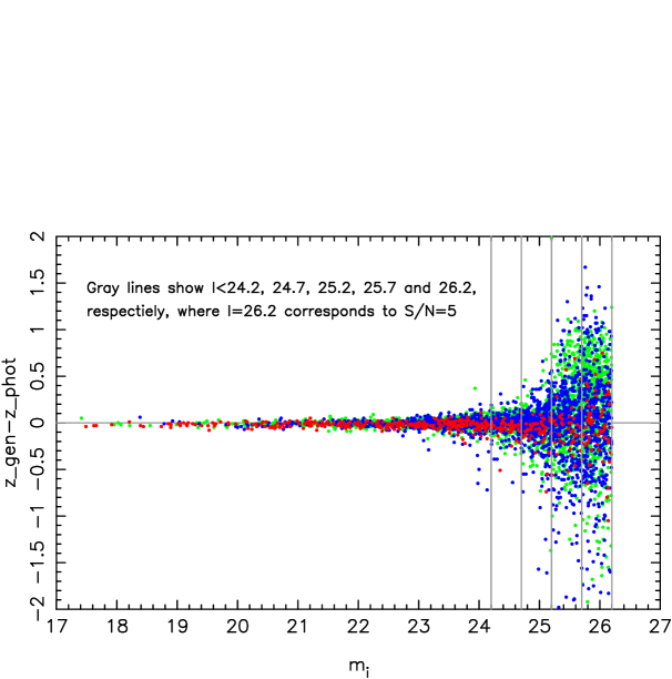
Figure 3: Simulation presenting the comparison between the input and output redshifts as a function of magnitude limit, S/N ratios and spectral types (elliptical (red), early/intermediate type spirals (green); late-type and starburst galaxies (blue).

Figure 3 shows comparison between the input and output redshifts as a function of i-band magnitude and $S/N$. At $i>25$ mag, the photometric redshift accuracy starts to significantly degrade. It is clear that at higher $S/N$ values (i.e. brighter $m_{i}$), photometric redshift code recovers the input redshifts. Also, most of the scatter at faint magnitudes (low S/N) is due to late-type galaxies and starbursts. This will be used as a guide to adopt the photometric or magnitude limit of the sample in order to optimise photometric redshift measurement.

4.2 Accuracy of photometric redshifts

The simulation results can be used to define a useful measure of the photometric redshift accuracy for each galaxy. This parameter is defined as

$$D_{95}={\Delta_{95}\over(1+z_{output})}$$

where $\Delta_{95}$ is the 95% confidence interval (i.e. the width of the redshift probability distribution corresponding to 95% confidence interval) and $z_{output}$ is the estimated photometric redshift. Therefore, $D_{95}$ can be calculated independent from any knowledge about spectroscopic redshift. If the error distribution is Gaussian, then, by definition, $\Delta_{95}=2\sigma_{z}$.

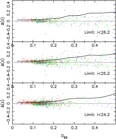
Figure 4: Simulation results for different magnitude limits demonstrating dependence of $D_{95}$ on $\Delta(z)$, which is a measure of the accuracy of the estimated photometric redshifts. The scatter in $\Delta(z)$ increases towards higher $D_{95}$ values and fainter magnitude limits. The black line shows variation in rms for $\Delta(z)$ as a function of $D_{95}$. For clarity, we only present the plots for $0<D_{95}<0.5$. A number of points on the $i<26.2$ panel scatter beyond the above $D_{95}$ and $\Delta(z)$ range, as they are undetected in the short wavelength bands and photometric redshift get less reliable . This is the reason for a relatively smaller number of points on the $i<26.2$ mag. panel.

To explore how $D_{95}$ is related to the accuracy of photometric redshifts, we study the correlation between $D_{95}$ with $\sigma(\Delta(z))$ and $\Delta(z)$, using the mock cataloge, as shown in Table 3 and Figure 4 respectively. The sample used in Table 3 is limited to galaxies with $S/N>10$. This is to minimise photometric uncertainties and to uncouple performance of different photometric redshift error estimators independent from photometric problems at faint flux levels. For simulated sub-samples, selected based on $D_{95}$ limits (Table 3; column 1), we estimate $\sigma(\Delta(z))$ values for the full sample and when excluding the outliers, defined as galaxies with $\Delta(z)>3\sigma(\Delta(z))$. Results are listed in Table 3, where it shows a clear decrease in $\sigma(\Delta(z))$ values and in fraction of the outliers towards smaller $D_{95}$. This demonstrates that $D_{95}$ provides a useful and practical measure to identify the fraction of outliers. Moreover, the median redshift of the survey is found to be independent of $D_{95}$, due to our $S/N$ cut.

The scatter in $\Delta(z)$ increases with increasing $D_{95}$ and for fainter magnitude limits. For galaxies with $D_{95}>0.2$, the scatter in $\Delta(z)$ significantly increases, indicating an increase in photometric redshift errors. For fainter galaxies ($i>24.2$ mag), where the accuracy of photometric redshifts decreases, we find an increase in $D_{95}$ parameter and larger scatter in $\Delta(z)$.

In summary, $D_{95}$ enables the identification of outliers in derived photometric redshifts, independent at all redshifts in the sample.

4.3 Comparison with Spectroscopic Redshifts

The ultimate test of the accuracy of photometric redshifts is the comparison with the spectroscopic redshifts. The spectroscopic sample here consists of galaxies observed to $i_{AB}\sim 24$ mag. in the $z$COSMOS program, using VIMOS on VLT (Lilly et al.  2006). We select 958 galaxies with the most reliable spectroscopic redshifts (based on two or three lines). We restrict the sample to redshift range $z<1.2$, as beyond this, the 4000 Å break lies at the edge of the optical bands. Also, due to the relatively shallow depth of our $K_{s}$-band data, these are not available for fainter galaxies. This reduces total number of galaxies with spectroscopic redshifts to 879.

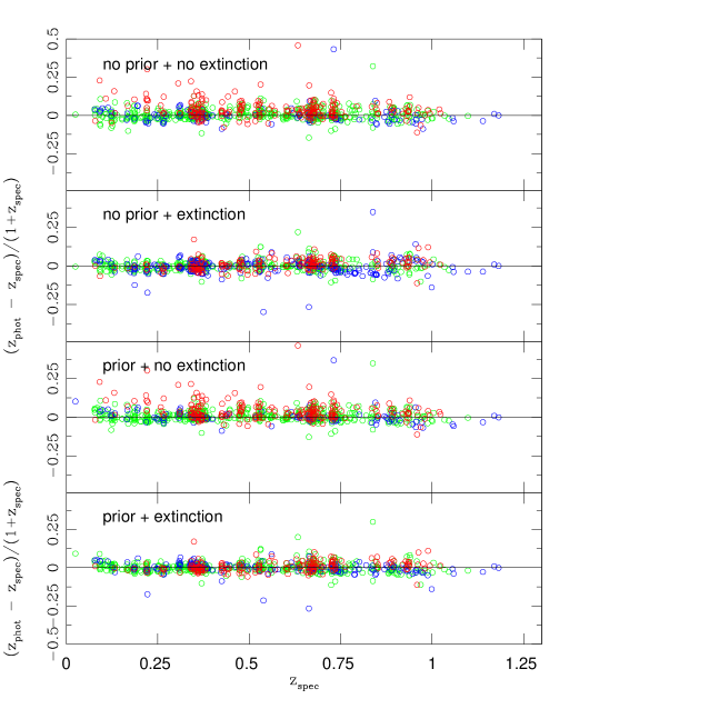
Figure 5: Comparison between photometric and spectroscopic redshifts for a sample of 958 galaxies in COSMOS with available spectroscopic redshifts. The colors correspond to elliptical (red), spiral (green) and starburst (blue) spectral types. The spectral types are evenly distributed with redshift, indicating no bias in spectral type classification as a function of redshift. The smallest scatter in $\Delta(z)$ ($(z_{phot}-z_{spec})/(1+z_{spec})$) obtained for the case including the prior and extinction.

Photometric redshifts were derived using the techniques described in §3 and compared with the spectroscopic redshifts in Figure 5. The effects of the luminosity function prior and extinction corrections are also explored. A total of 12 galaxies in the spectroscopic sample ($z<1.2$) were identified as AGNs from their X-ray emission (Brusa et al.  2006). The AGNs were removed from the spectroscopic sample and only the “normal” galaxies were used in the comparison.

We measure the $D_{95}$ parameter for the 868 galaxies with $z<1.2$ in our spectroscopic sample. The relation between $D_{95}$ and $\Delta(z)=(z_{phot}-z_{spec})/(1+z_{spec})$ is shown in Figure 6a. Galaxies with $D_{95}<0.2$ are seen to have, on average, $\Delta(z)\sim 0$ although with some scatter. This confirms that, on average, $D_{95}$ parameter provides a good measure of the reliability of photometric redshifts. Distribution of $D_{95}$ values for three spectral types of galaxies (elliptical, spiral and starbursts) in the spectroscopic sample are presented in Figure 6b. The width of the distributions for different types are consistent with the observed scatter in Figure 6a. The peak of the $D_{95}$ distributions are at $D_{95}\sim 0.08$ (for ellipticals) and 0.12 (for spirals and starbursts), indicating the reliability with which one could measure photometric redshifts for different spectral types of galaxies.

Table 4 compares the $\sigma(\Delta(z))$ values and the fraction of outliers, defined as objects with $\Delta(z)>3\sigma(\Delta(z))$, for different cases (with and without prior and extinction). It is clear from Table 4 and Figure 5 that the best agreement between the photometric and spectroscopic redshifts are obtained when both prior and extinction corrections are enabled. In its best case, this corresponds to an rms of $\sigma(\Delta(z))=0.031$. This is consistent with the rms estimated from the simulations in §3. It is also clear from Table 4 that $D_{95}$ parameter is directly correlated with the fraction of outliers, as defined by $\sigma(\Delta(z))$- (i.e. deviation of photometric redshift from its spectroscopic counterpart). No trend is found between redshift and spectral types in Figure 5, indicating there is no significant bias in redshift estimates as a function of spectral type.

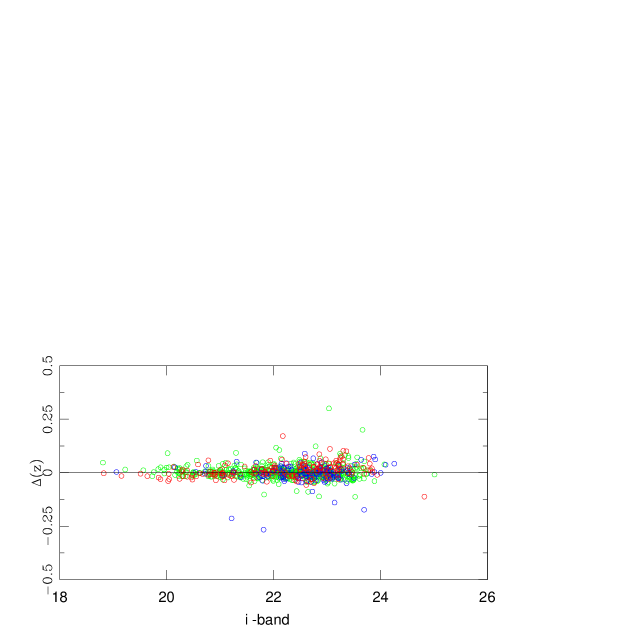
Figure 7: Changes in $\Delta(z)=(z_{spec}-z_{phot})/(1+z_{spec})$ as a function of $i-$ band magnitudes. There is slight increase in the scatter in $\Delta(z)$ (more uncertain photometric redshifts) at $i>23$.

Finally, the relation between $\Delta(z)$ and i-band magnitudes for “normal” galaxies in the spectroscopic sample is shown in Figure 7. The errors in the photometric redshift shows no dependance on the magnitude of the galaxies or their spectral type.

We divide galaxies into spectral type bins (ellipticals, spirals and starbursts) and compare their estimated photometric and spectroscopic redshifts, as listed in Table 4. The photometric redshifts are estimated for the case assuming prior and extinction (the optimum case), considering all galaxies regardless of their $D_{95}$. We find comparable $\sigma(\Delta(z))$ values for elliptical (0.034), spiral (0.030) and starbursts (0.042). For each of the scenarios in Table 4, we also estimate the fraction of galaxies (with respect to total) of different spectral types. The result, listed in Table 4, shows a simultaneous decrease in the fraction of ellipticals and increase in the fraction of starbursts when extinction correction is enabled. No significant change in the fraction of spirals is observed.

Figure 5 shows a reduction in $\sigma(\Delta(z))$ for ellipticals when extinction correction is applied, with this having a less significant effect for the starbursts, contrary to expectations. However, as shown in Table 4, we find a change in the fraction of both ellipticals and starbursts when dust extinction is included as a free parameter in the photometric redshift fits. This indicates a change in the best-fit spectral types of galaxies (Figure 5), depending wether or not we apply the dust extinction correction. The derived spectral types of elliptical and later type (spirals, irregulars and starbursts) galaxies here are examined by comparing them with independently estimated quantitative morphologies (compactness, asymmetry and Gini coefficients). These morphological parameters are consistent with the derived spectral types (Capak et al.  2006).

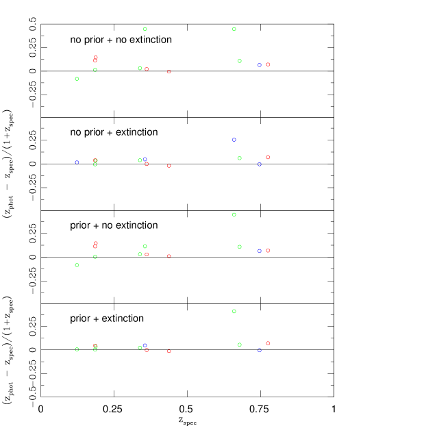
Figure 8: The same as in Figure 5 but for 12 spectroscopically identified AGNs.

We now estimate photometric redshifts for 12 AGNs with $z<1.2$, including the prior and extinction. These are compared with their spectroscopic redshifts in Figure 8 and show that the rms scatter is again lowest when including the prior and correcting for local extinction. This corresponds to $\sigma(\Delta(z))=0.10$ (Table 4). The small rms measured for AGNs (type II) indicates that once extinction fitting is enabled, one can derive their photometric redshifts using templates based on normal galaxies.

5 Other Photometric Redshift Codes

In this section we explore how photometric redshifts depend on different techniques, codes and choice of priors, using a variety of photometric redshift codes. We compare results from the code presented in the previous section (refered to as ”COSMOS”) with three other codes: Zurich Extragalacitc Bayesian Redshift Analyzer (ZEBRA; Feldmann et al. 2006), Le Phare (Arnout 1999) and Baysian Photometric Redshift code (BPZ; Benitez 2000). Here we give a summary of basic characteristics of these codes.

The Zurich Extragalactic Baysian Redshift Analyzer (ZEBRA): ZEBRA estimates redshifts and template types of galaxies using medium- and broad-band photometric data (Feldmann et al.  2006). In the photometry check mode, for each galaxy and in any given filter, ZEBRA computes the difference between the observed magnitudes and those predicted by templates, using a training set with available spectroscopic redshifts. A linear (or higher order) regression is then applied to the relation between the residual and observed galaxy magnitude, with a constant offset estimated and subsequently applied to magnitudes in any given filter. In the template check mode, ZEBRA uses the $\chi^{2}$ minimization technique to optimize the difference between the observed and template-based fluxes for all passbands, averaged over all galaxies in the photometric catalog. By introducing additional terms to the $\chi^{2}$ equation, ZEBRA prevents too large deviations between the observed and model templates and regularizes the template shapes. It is run in both Maximum Likelihood and Baysian modes. In the later case, a prior is calculated in redshift and template space, using an iterative procedure. In the current release of this code, reddening due to dust extinction is not included.

Le Phare photometric redshift code: The Le Phare code (Arnouts et al. 1999) is based on $\chi^{2}$ fitting method, comparing the observed magnitudes with those predicted from an SED library. This simultaneously runs libraries for stars, galaxies and quasars, which are then used to separate different classes of objects. An automatic calibration method is applied by using the spectroscopic redshift sample as training set (Ilbert et al.  ., 2006). This adaptive method combines an iterative correction of the photometric zero-points and an optimisation of the SED templates. It allows to remove systematic differences between the spectroscopic and photometric redshifts and reduce the fraction of catastrophic failures. Reddening correction is applied to templates later than Sbc types, using the small Magellanic cloud extinction law. In this work, we adopt the same empirical templates as Ilbert et al. (2006). An additional Bayesian approach has been used, involving priors based on redshift distributions, following the formalism of Benitez (2000).

Baysian Photometric Redshift Code (BPZ): The Bayesian approach considers the redshift distribution, $p(z|C,m)$, as a function of the observed color ($C$) and magnitude ($m$)- (Benitez 2000). The prior used here is therefore based on the probability of a galaxy having redshift, $z$, and spectral type, $T$, given its magnitude. This is different from a luminosity function based prior used in the previous sections (the COSMOS code). Therefore the BPZ code provides redshifts based on both maximum liklihood and prior based techniques. The prior-based photometric redshifts from the BPZ are generally found to be more accurate than the results obtained when no priors are used.

The four codes are not completely identical and hence, we need to specify any intrinsic differences between them when comparing results from the codes. We present a list of the set up parameters used in each of the above codes in Table 5.

5.1 Comparison between different photometric redshift codes

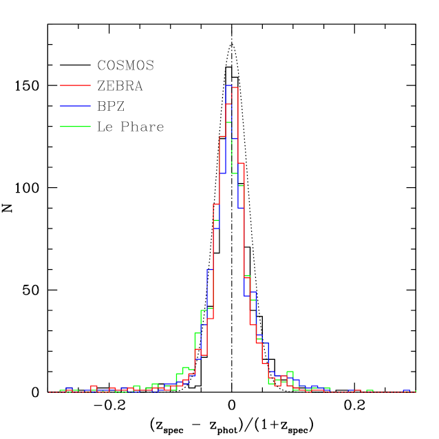
Figure 9: Distribution of $\Delta(z)=(z_{spec}-z_{phot})/(1+z_{spec})$ values from COSMOS, Le Pahre, ZEBRA and BPZ photometric redshift codes. All follow a Gaussian distribution with a peak at $\Delta(z)\sim 0$. The distributions are best fit with a Gaussian with $\sigma=0.026$. Photometric redshifts are estimated assuming no priors.

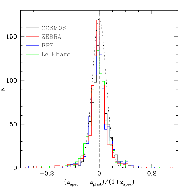
Figure 10: The same as Figure 9 but assuming priors in estimating photometric redshifts.

The four photometric redshift codes have been applied on the same spectroscopic sample, with the $\Delta z=(z_{phot}-z_{spec})/(1+z_{spec}$) distributions compared in Figures 9 (without prior) and 10 (with prior). The $\Delta z$ distributions from the codes used here are approximately fitted by a Gaussian with $\sigma=0.026$ (Figures 9 and 10). However, the distributions for some codes are slightly offset from $\Delta z=0$, with extended wings.

The absolute accuracy in each code depends on the way the outliers are defined. To directly compare the photometric redshift accuracy from various codes, we follow the same procedure for all the four photometric redshift codes and present the results in Table 6 (with no priors) and Table 7 (with priors). For each code, we calculate the upper and lower 68% intervals (top-left and top-right number in each grid) from the distribution of $\Delta(z)$ between the photometric and spectroscopic redshifts and between the photometric redshifts from different codes. This is a different definition than the “average” rms values presented for COSMOS photometric redshifts in Table 4 and is defined to more clearly show the asymmetry in $\Delta(z)$ distributions between different codes. This also explains the difference in the scatter between photometric and spectroscopic redshifts found here (Tables 6 and 7) compared to that listed in Table 4.

Assuming a Gaussian distribution for $\Delta(z)$ values, that would correspond to 1$\sigma$ standard deviation and for symmetric distributions the top-left and the top-right number should be the same. Objects with $\Delta(z)$ values outside the 1$\sigma$ limit (bold number in each grid in Tables 6 and 7) are considered as outliers. This prescription defines the accuracy independent of the definition of the outliers.

The comparison between the estimated redshifts from various photometric redshift codes with their spectroscopic counterparts are also shown on the first row of Tables 6 and 7. The rest of the entries present comparison between the different codes. Results listed in the tables show excellent agreement between different photometric redshift codes, with all agreeing well with the spectroscopic redshifts. However, there is a slight improvement in the rms scatter for COSMOS code when using the prior while, prior has no such effect on other codes. This is likely due to the fact that the prior here was partly optimised on the spectroscopic data, using the photometric data set.

6 Analysis of Photometric data

In the previous sections we demonstrated that one could derive reliable photometric redshifts, using the available multi-waveband data for galaxies in COSMOS. These are extensively used in the analysis of COSMOS dataset. In this section we present preliminary results, using the photometric redshifts for the entire COSMOS galaxies with $i<25$ mag. Given the results in Table 4, we use prior and consider extinction as an independent parameter in the fit.

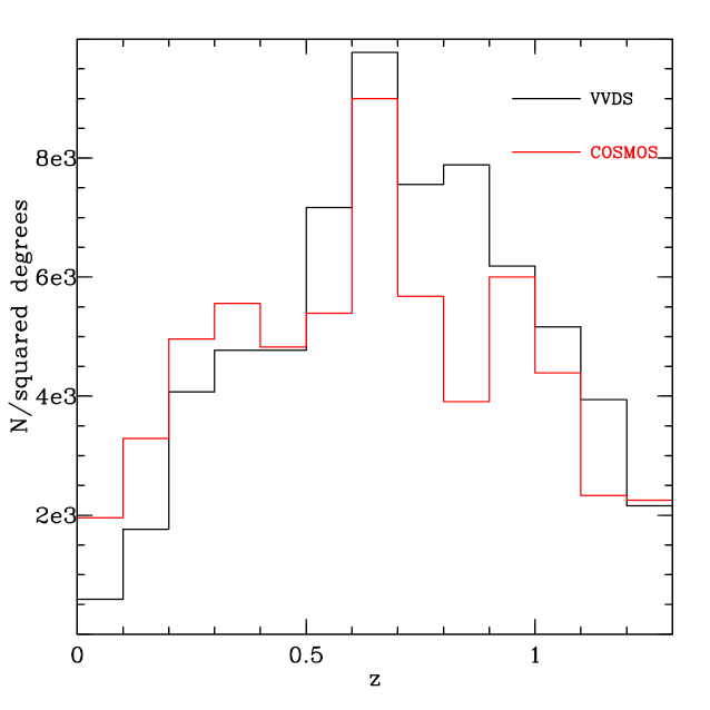
Figure 12: Comparison between photometric redshift distribution from COSMOS and spectroscopic redshift distribution (from VVDS). Galaxies to $i_{AB}\sim 24$ are used.

The photometric redshift distributions for different spectral types of galaxies in COSMOS are presented in Figure 11. Only galaxies with $i<25$ mag are used here, as they have the most reliable photometric redshifts. Moreover, as discussed in §4.3, we restrict the sample to galaxies with $z<1.2$. There is similar distribution for all the spectral types with redshift. The photometric redshift distribution for COSMOS (to $i_{AB}<24$) is compared in Figure 12 with the spectroscopic redshift distribution for the VVDS to the same depth (Le Fevre et al. 2005), after normalising the number of sources to the areas of their respective surveys. The overall agreement is good, with similar median redshifts. The VVDS only targets 25% of the galaxies to its spectroscopic magnitude limit. This, combined with the difficulty in measuring spectroscopic redshifts for fainter galaxies in VVDS and cosmic variance are responsible for the observed difference between the two distributions in Figure 12.

In Figure 13 we present rest-frame absolute magnitudes ($M_{V}$) for COSMOS galaxies. These are estimated using its best-fit photometric redshift and spectral type, following the prescription described in Dahlen et al.  (2005). As expected, there is a trend in $M_{V}$ absolute magnitudes with spectral types, with objects with earlier types being brighter. The median absolute magnitudes correspond to $M_{V}=-21.3$ (E/SO), $-20.5$ (Sa/Sb), $-19.7$ (Sc), $-18.7$ (starbursts).

6.1 Stellar Mass Estimates

The stellar mass for COSMOS galaxies is measured using the relation between $M/L_{V}$ and rest-frame $(B-V)_{0}$ colors

$$M/L_{V}=-0.628+1.305\ (B-V)_{0}$$

Bell et al.  (2005). We assume Salpeter IMF with $0.1M_{\odot}<M<100M_{\odot}$. Average rest-frame $<B-V>_{0}$ colors, corrected for extinction, are estimated for each spectral type (E, Sa, Sb, Sc, Im and starburst), using the appropriate templates. Then, to each galaxy, using its best-fit spectral type (which is derived consistently with its estimated extinction and photometric redshift), we assign the $<B-V>_{0}$ color and hence, the $M/L_{V}$ ratio from the above equation. Combined with rest-frame absolute V-band magnitudes ($M_{V}$), the stellar mass is then estimated as

$$log(M_{stellar}/M_{\odot})=M/L_{V}-0.4\ (M_{V}-4.82)$$

K-band luminosities, being produced by evolved stellar population in galaxies, are more directly correlated with the stellar mass in galaxies. However, due to shallowness of our K-band data over the COSMOS area, many galaxies are not detected in this band. Therefore, we use the V-band luminosity as a proxy for the K-band to measure the stellar mass. For a sub-set of our galaxies, the stellar masses measured using the K- and V- band luminosities were compared and agree better than 5%. However, by definition, this is a sample dominated by the most massive and reddest galaxies and therefore, this cannot be used as a measure of the accuracy for stellar masses for the rest of the galaxies in this sample. The main source of uncertainty in our stellar mass estimates here is the scatter in the mean $<B-V>_{0}$ colors for each spectral type and the accuracy with which the spectral types are measured for individual galaxies.

In Figure 14 we present the distribution of $M_{stellar}/M_{\odot}$ values as a function of spectral type and redshift. In a given redshift range, elliptical and early-type spiral galaxies are more massive than later type galaxies. However, for a given spectral type of galaxies, we find an increase in galaxy mass with redshift. This is likely caused by a bias in our magnitude limited sample, due to selecting brighter galaxies at higher redshifts.

7 Summary

We develop a photometric redshift code and use that to measure redshifts and spectral types for galaxies in the COSMOS survey. The technique uses $\chi^{2}$ template fitting, combined with luminosity function priors and with the option to estimate internal extinction ($E(B-V)$). We use extensive simulations to examine reliability of the code and study its accuracy as a function of photometric magnitude limits and $S/N$ ratios. We define a new parameter, $D_{95}$, to identify the objects with catastrophic failure in photometric redshift estimate.

We estimate photometric redshifts for a sample of 868 galaxies with available spectroscopic redshifts (to $z<1.2$) from $z$COSMOS. Considering different scenarios, dependeing on using prior and/or extinction, we compare the photometric and spectroscopic redshifts for this sample. The best agreement is found when invoking both prior and dust extinction correction, giving $\sigma(\Delta(z))=0.031$, where $\Delta(z)=(z_{phot}-z_{spec})/(1+z_{spec})$. This gives a small fraction of outliers (2.5%). For a sample of 12 type II AGNs with available spectroscopic redshifts, we find $\sigma(\Delta(z))=0.10$.

Our photometric redshift code here is compared with three independent codes. The estimated redshifts are in excellent agreement. We measure photometric redshifts and spectral types for the entire COSMOS galaxies and present preliminary results concerning redshift and absolute magnitude distributions. We use the estimated photometric redshifts and spectral types to measure stellar masses of galaxies and study changes in stellar mass among galaxies with different spectral types and with redshift.

Table 1: Data Quality and Depth

Filter	Central	Filter	Seeing	Depth	Saturation	Offset from
Name	Wavelength (Å)	Width (Å)	Range (′′ )		Magnitude	Vega System
$u^{\prime}$	3591.3	550	1.2-2.0	22.0	12.0	0.921
$u^{*}$	3797.9	720	0.9	26.4	15.8	0.380
$B_{J}$	4459.7	897	0.4-0.9	27.3	18.7	-0.131
$g^{\prime}$	4723.1	1300	1.2-1.7	22.2	12.0	-0.117
$g^{+}$	4779.6	1265	0.7-2.1	27.0	18.2	-0.117
$V_{J}$	5483.8	946	0.5-1.6	26.6	18.7	-0.004
$r^{\prime}$	6213.0	1200	1.0-1.7	22.2	12.0	0.142
$r^{+}$	6295.1	1382	0.4-1.0	26.8	18.7	0.125
$i^{\prime}$	7522.5	1300	0.9-1.7	21.3	12.0	0.355
$i^{+}$	7640.8	1497	0.4-0.9	26.2	20.0	0.379
$i^{*}$	7683.6	1380	0.94	24.0	16.0	0.380
$F814W$	8037.2	1862	0.12	24.9	18.7	0.414
$NB816$	8151.0	117	0.4-1.7	25.7	16.9	0.458
$z^{\prime}$	8855.0	1000	1-1.7	20.5	12.0	0.538
$z^{+}$	9036.9	856	0.5-1.1	25.2	18.7	0.547
$K_{s}$	21537.2	3120	1.3	21.6	10.0	1.852

Table 2: Photometric redshift accuracy from the COSMOS simulations for different limiting magnitudes. Outliers here are defined as objects with $\Delta(z)>3\sigma(\Delta(z))$, where $\Delta(z)=(|z_{output}-z_{input}|)/(1+z_{input})$.

$m_{lim}$	$\sigma(\Delta(z))$	$\sigma(\Delta(z))$	Fraction of	Median z	Fraction types
	full sample	w/o outliers	outliers (%)		(%)
$<26.2$	0.183	0.140	2.1	1.13
$<25.7$	0.142	0.088	2.2	0.96
$<25.2$	0.089	0.048	1.1	0.81
$<24.7$	0.054	0.031	0.62	0.73
$<24.2$	0.042	0.025	0.37	0.67
$i<25.2$:
early-type	0.058	0.031	0.40	0.90	14
late-type	0.085	0.045	0.83	0.78	60
starburst	0.11	0.065	1.1	0.84	26

Table 3: Relation between $D_{95}$ and the photometric redshift accuracy ($\sigma(\Delta(z))$) from the COSMOS simulations only using objects with S/N $>$ 10. The outliers here are defined as objects with $\Delta(z)>3\sigma(\Delta(z))$ and are measured for the samples selected based on $D_{95}>D_{95}^{0}$, where $D_{95}^{0}$ values are listed in column 1.

$D_{95}$	Spectral	$\sigma(\Delta(z))$	$\sigma(\Delta(z))$	Fraction of	Median z	Fraction of
	types	full sample	w/o outliers	outliers (%)		objects (%)
all objects	all	0.114	0.066	1.5	0.91	100
	early	0.061	0.034	0.57	0.93	12
	late	0.11	0.062	1.6	0.84	60
	starburst	0.14	0.084	1.5	0.92	28
$<0.7$	all	0.056	0.042	2.1	0.96	83
	early	0.034	0.028	1.8	0.95	14
	late	0.053	0.040	1.9	0.86	59
	starburst	0.072	0.055	2.5	0.92	27
$<0.5$	all	0.041	0.033	1.7	0.93	72
	early	0.034	0.028	1.8	0.94	16
	late	0.038	0.032	1.8	0.81	60
	starburst	0.049	0.039	1.5	0.84	24
$<0.3$	all	0.030	0.026	0.80	0.82	58
	early	0.027	0.024	1.3	0.89	18
	late	0.027	0.025	1.1	0.72	60
	starburst	0.038	0.028	2.5	0.65	22

Table 4: Comparison with spectroscopic redshifts. Outliers here are defined the same as in Table 3

$D_{95}$	$\sigma(\Delta(z))$	$N_{tot}$	$N_{outlier}$	Outlier fraction	$n_{E}$	$n_{sp}$	$n_{Starburst}$
no prior + no extinction corr.
all	0.091 (0.042)	868	5	0.006	0.25	0.63	0.12
$<0.2$	0.047 (0.035)	828	18	0.022
$<0.3$	0.047 (0.035)	841	19	0.023
no prior + extinction corr.
all	0.086 (0.034)	868	4	0.005	0.20	0.52	0.28
$<0.2$	0.036 (0.029)	779	15	0.019
$<0.3$	0.036 (0.029)	830	15	0.018
with prior + no extinction corr.
all	0.17 (0.047)	868	5	0.006	0.24	0.65	0.11
$<0.2$	0.044 (0.033)	841	18	0.021
$<0.3$	0.045 (0.033)	845	19	0.022
with prior + with extinction corr.
all	0.033 (0.025)	868	19	0.022	0.20	0.63	0.17
$<0.2$	0.031 (0.025)	838	15	0.018
$<0.3$	0.031 (0.025)	846	16	0.019
with prior + with extinction corr.
Ellipticals	0.034 (0.028)	174	5	0.029
Spirals	0.030 (0.023)	543	10	0.018
Starbursts	0.042 (0.027)	151	4	0.026
AGNs	0.10 (0.026)	12	1	0.083

Table 5: List of the initial parameters used for different codes

	without priors			with priors
	ML	SED optimization	Reddening	Baysian	SED optimization	Reddening
BPZ	X	X	–	X	X	–
COSMOS	Best $\chi^{2}$	X	X	X	X	X
Le Phare	X	X	X	X	X	X
ZEBRA	X	X	–	X	X	–

Table 6: Accuracy of the codes with no priors compared to the spectroscopic sample and compared with the others

no priors	COSMOS		Le Phare		BPZ		ZEBRA
	-0.030	0.028	-0.024	0.032	-0.030	0.027	-0.022	0.024
Zspec	0.029		0.028		0.029		0.023
			-0.026	0.036	-0.026	0.026	-0.027	0.024
COSMOS			0.031		0.026		0.026
					-0.026	0.019	-0.027	0.023
Le Phare					0.022		0.025
							-0.022	0.020
BPZ							0.021

Table 7: Accuracy of the codes whit priors compared to the spectroscopic sample and compared with the others

priors	COSMOS		Le Phare		BPZ		ZEBRA
	-0.025	0.024	-0.025	0.031	-0.030	0.026	-0.020	0.026
Zspec	0.025		0.028		0.028		0.023
			-0.030	0.022	-0.020	0.021	-0.024	0.014
COSMOS			0.026		0.021		0.019
					-0.017	0.024	-0.025	0.024
Le Phare					0.020		0.024
							-0.025	0.016
BPZ							0.020

Figure 6: (a). Changes in $D_{95}$ parameter as a function of $\Delta(z)=(z_{phot}-z_{spec})/(1+z_{spec})$ for the spectroscopic sample. Galaxies with $D_{95}<0.2$ have more accurate photometric redshifts, as shown by the dotted line- Ellipticals (red), Spirals (green), starbursts (blue). (b). Distribution of $D_{95}$ parameter for the spectroscopic sample. Different spectral types are identified with the color code as above.

Figure 11: Photometric Redshift distributions for different spectral types of galaxies for the entire COSMOS galaxies with $i<25$. The distributions for each spectral type are normalized to the total number of galaxies with that spectral type.

Figure 13: Rest-frame absolute magnitude distributions for different spectral types of galaxies in the entire COSMOS catalog. The expected trend is present, with early-type galaxies having brighter absolute magnitudes. The distributions for each spectral type are normalized to the total number of galaxies with that spectral type.

Figure 14: Distribution of stellar mass as a function of spectral type and redshift for galaxies in the COSMOS survey

References

- (1) Arnouts, S.; Cristiani, S.; Moscardini, L.; Matarrese, S.; Lucchin, F.; Fontana, A.; Giallongo, E. 1999, MNRAS 310, 540
- (2) Bell, E. et al. . 2005, ApJ 625, 23
- (3) Benitez, N. 2000, ApJ. 536, 571
- (4) Bolzonella, M.; Miralles, J.-M.; Pello, R. 2000 A& A 363, 476
- (5) Bundy, K.; Ellis, R. S.; Conselice, C. J. 2005, ApJ, 625, 621
- (6) Capak, P., Mobasher, B., Abraham, B., Sheth, K., Scoville, N. Z. & Ellis, R. S. 2006 ApJ Suppl. This issue
- (7) Capak, P. et al. 2004 AJ 127, 180
- (8) Caputi, K. I.; Dunlop, J. S.; McLure, R. J.; Roche, N. D. 2005, MNRAS 361, 607
- (9) Carollo, M. et al. . 2006 ApJ Suppl (this issue)
- (10) Daddi, E. et al. . ApJ 2005, 631, 13
- (11) Calzetti, D.; Armus, L.; Bohlin, R. C.; Kinney, A. L.; Koornneef, J.; Storchi-Bergmann, T. 2000 ApJ. 533, 682
- (12) Coleman, G. D.;, Wu, C. C.; & Weedman, D. W. 1980, ApJS. 43, 393
- (13) Cowie, L. L.; Barger, A. J.; Hu, E. M.; Capak, P.; Songaila, A. AJ 127, 3137
- (14) Dahlen, T., Mobasher, B., R. S. Somerville, Moustakas, L. A., Dickinson, M. 2005 ApJ 631, 126
- (15) Dahlen, T., Mobasher, Dickinson, M., Ferguson, H. C., Giavalisco, M. 2006, ApJ submitted
- (16) Drory, N.; Salvato, M.; Gabasch, A.; Bender, R.; Hopp, U.; Feulner, G.; Pannella, M. 2005 ApJ 619, L131
- (17) Ferguson, H. C. & Giavalisco, M. 2005, ApJ. 631, 126
- (18) Feulner, Georg; Gabasch, Armin; Salvato, Mara; Drory, Niv; Hopp, Ulrich; Bender, Ralf 2005, ApJ 633, L9
- (19) Erb, D. K.; Steidel, C. C.; Shapley, A. E.; Pettini, M.; Adelberger, K. L. 2004, ApJ, 612, 122
- (20) Giavalisco, M. et al. . 2004, ApJL 600, L93
- (21) Gwyn, S. D. J.; Hartwick, F. D. A. 1996, ApJ 468, 77
- (22) Ilbert, O. et al. 2006 (in press) astro-ph 0409134
- (23) Kinney, A. L., Calzetti, D., Bohlin, R. C., McQuade, K., Stori-Bergmann, T., Schmitt, H. R. 1996, ApJ. 467, 38
- (24) Landolt, A. U., 1992, AJ, 104,340
- (25) Lilly, S. et al. 2006 ApJ. Suppl. (this issue) Mobasher, B., Rowan-Robinson M., Georgakakis A., & Eaton, N. 1996, MNRAS, 282, L7
- (26) Maraston, C., 2005, MNRAS, 362, 799
- (27) Mobasher, B. et al. . 2004, ApJL. 600, 167
- (28) Mobasher, B. et al. . 2005, Ap. J. 635, 832
- (29) Pannella, M.; Hopp, U.; Saglia, R. P.; Bender, R.; Drory, N.; Salvato, M.; Gabasch, A.; Feulner, G. 2006 ApJ 639, L1
- (30) Papovich, C. et al. . 2006, Ap. J. 640, 92
- (31) Scarlata et al. . 2006 ApJ Suppl. (this issue)
- (32) Scoville, N. Z. et al. . 2006 ApJ Suppl. (this issue)
- (33) Steidel, C. C.; Shapley, A. E.; Pettini, M.; Adelberger, K. L.; Erb, D. K.; Reddy, N. A.; Hunt, M. P. 2004, ApJ, 604, 534
- (34) Treu, T.; Ellis, R. S.; Liao, T. X.; van Dokkum, P. G.; Tozzi, P.; Coil, A.; Newman, J.; Cooper, M. C.; Davis, M. 2005, ApJ, 663,174
- (35) Wang et. al., 2005, astro-ph, 0512347
- (36) Wolf, C., Meisenheimer, K., Rix, H. -W., Borch , A., Dye, S., & Kleinheinrich, M. 2003, A&A, 401, 73
- (37) Wirth, G. D. 2004 AJ. 127, 3121
- (38) Yan, H. et al. 2005, ApJ. 634, 109