The XMM-Newton Survey in the Marano Field

We report on a medium deep XMM-Newton survey of the Marano Field and optical follow-up observations. The mosaicked XMM-Newton pointings in this optical quasar survey field cover 0.6 deg² with a total of 120 ksec good observation time. We detected 328 X-ray sources in total. The turnover flux of our sample is $f_{\rm{X}}\sim 5\times 10^{-15}$ erg cm^-2 s^-1 in the 0.2-10 keV band. With VLT FORS1 and FORS2 spectroscopy we classified 96 new X-ray counterparts.

The central 0.28 deg², where detailed optical follow-up observations were performed, contain 170 X-ray sources (detection likelihood $ML>10$), out of which 48 had already been detected by ROSAT. In this region we recover 23 out of 29 optically selected quasars. With a total of 110 classifications in our core sample we reach a completeness of $\sim$65%. About one third of the XMM-Newton sources is classified as type II AGN with redshifts mostly below 1.0. Furthermore, we detect five high redshift type II AGN ($2.2\leq z\leq 2.8$).

We show that the true redshift distribution of type II AGN remains uncertain, since their lack of emission lines in a wide optical wavelength range hampers their identification in the redshift range $1<z<2$. The optical and X-ray colors of the core sample indicate that most of the still unidentified X-ray sources are likely to be type II AGN. We calculate absorbing column densities and show that the ratio of absorbed to unabsorbed objects is significantly higher for type II AGN than for type I AGN. Nevertheless, we find a few unabsorbed type II AGN. The X-ray hardness ratios of some high redshift type I AGN also give an indication of heavy absorption. However, none of these type I objects is bright enough for spectral extraction and detailed model fitting. Type I and II AGN cover the same range in intrinsic X-ray luminosity, ($10^{43}\leq L_{\rm{X}}\leq 10^{46}$), although type II AGN have a lower median intrinsic X-ray luminosity (log $L_{\rm{X}}\sim 44.0$) compared to type I AGN (log $L_{\rm{X}}\sim 44.4$).

Furthermore, we classified three X-ray bright optically normal galaxies (XBONGs) as counterparts. They show properties similar to type II AGN, probably harbouring an active nucleus.

1 Introduction

X-ray surveys are essential to characterize the source population of the X-ray sky and are the only means to understand the nature of the X-ray background radiation. Deep X-ray surveys had been carried out during the last decades (Hasinger et al. 1998, Lehmann et al. 2001, Alexander et al. 2003) and showed that up to 80% of the soft X-ray background is due to active galactic nuclei (AGN). XMM-Newton and CHANDRA, thanks to their high sensitivity at hard X-rays, opened the absorbed X-ray universe for further studies and revealed a large population of obscured, low-luminosity, low-redshift X-ray sources (Hasinger et al. 2001).

In order to characterize the X-ray sky properly and understand the X-ray background peak at $\sim$30 keV (Worsley et al. 2005) numerous surveys with a large variety in limiting flux and survey area are needed (see Fig. 1 in Brandt & Hasinger 2005). In this paper, we present new XMM-Newton data and spectroscopic classifications of X-ray sources in the Marano Field.

The Marano Field was named by an early optical quasar survey up to a limiting magnitude of $B_{\rm{J}}=22.0$ by Marano et al. (1988). Based on different optical selection techniques (color-color diagrams, grism plates, variability analysis) they discovered 23 broad emission line quasars and defined an extensive list of quasar candidates. Zitelli et al. (1992) completed this work by presenting a spectroscopically complete sample of quasars with $B_{\rm{J}}\leq 22.0$ using this list of quasar candidates. They confirmed 54 quasars including the former 23 quasars. Between December 1992 - July 1993 ROSAT observed the central Marano Field ($\sim$0.2 deg²) for 56 ksec (Zamorani et al. 1999). The data revealed 50 X-ray sources with a limiting flux of $f_{\rm{X}}\geq 3.7\times 10^{-15}\,$erg cm^-2 s^-1 in the ROSAT band (0.5-2.0 keV). Multi-color CCD and spectroscopic data identified 42 X-ray sources (33 quasars, 2 galaxies, 3 clusters, and 4 stars). 66% of the optically selected quasars within the ROSAT field-of-view were detected as ROSAT X-ray sources. Gruppioni et al. (1999) carried out a deep radio survey at 1.4 and 2.4 GHz and detected 68 radio sources ($f_{\rm{R}}>0.2$ mJy). Follow-up observation provided redshifts for 30 objects.

Our new XMM-Newton data comprise a three times larger area compared to the ROSAT survey and are thus almost comparable in size to the optical quasar survey. We are reaching a survey sensitivity of $f_{\rm{X}}\sim 5\times 10^{-15}\,$erg cm^-2 s^-1 (turnover flux) over a contiguous area of 0.6 deg². The XMM-Newton survey of the Marano Field is thus comparable with deep ROSAT surveys (e.g. the UDS, Hasinger et al. 1998) or with medium deep CHANDRA surveys (e.g. ChaMP, Green et al. 2004).

The paper is organized as follows. In Sect. 2 we list the X-ray and optical data and the reduction of the data. Sect. 3 describes and summarizes the spectroscopic classification of the X-ray sources.

In Sect. 4 we make use of the spectroscopic classification and redshift determination to analyze the properties of different object classes. In this section we concentrate on a ’core sample’ of objects in the central part of the field, where we reached the highest degree of completeness in the spectroscopic classification.

Sect. 5 addresses additional objects in the Marano Field that are not X-ray detected. These objects were obtained as a control sample. Sect. 6 dicusses the results on the different object classes. Finally, our conclusions are outlined in Sect. 7.

Unless mentioned otherwise, all errors refer to a $68\%$ confidence interval.

2 Observations and data reduction

2.1 XMM-Newton X-ray observations

Since the area of the optical quasar survey in the Marano Field is larger than the XMM-Newton field of view, the X-ray observations have been performed as a grid of $4\times 4$ overlapping pointings with a spacing of $\sim$5 arcmin in right ascension and declination. The pointing in the north-western corner of the grid was shifted in order to cover the position of a deep far-infrared survey with the ISO satellite (Table 1 and Fig. 1). The ISO data are not addressed in this paper.

Table 1: XMM-Newton observations of the Marano Field. Filter: T.-thin, M.-medium.

XMM-orbit/	date	RA	DEC	time	filter
ObsID	(2000)	(3h:min:ss)	(-55:min:ss)	(ks)
106/0112940201	7/7	15:27	06:13	10.3	T.
107/0112940201	10/7	16:03	21:41	10.4	T.
107/0112940301	10/7	15:27	11:22	10.6	T.
107/0112940401	10/7	15:27	16:32	10.5	T.
107/0112940501	10/7	15:27	21:41	7.8	T.
129/0129321001	22/8	16:03	11:22	6.1	T.
129/0129320801	22/8	16:03	16:32	10.6	M.
129/0129320901	22/8	16:03	06:13	10.6	T.
130/0110970101	24/8	13:09	03:54	10.9	T.
130/0110970201	24/8	14:15	11:22	9.1	T.
130/0110970301	24/8	14:15	16:32	9.1	T.
130/0110970401	24/8	14:15	21:41	9.1	T.
131/0110970501	26/8	14:51	06:13	9.1	T.
131/0110970601	26/8	14:51	11:22	9.9	T.
133/0110970701	30/8	14:51	16:32	9.9	T.
133/0110970801	30/8	14:51	21:41	8.8	T.

Due to the overlapping pointings some deviations from the standard XMM-Newton data analysis procedures were necessary, which are described here.

The photon event tables from the 16 grid pointings were merged into a single event table with a common sky coordinate frame using the XMM SAS merge task. In this coordinate frame we created 240 images (one for each pointing, energy range, and instrument). The 5 bands used are 0.2-0.5 keV, 0.5-2.0 keV, 2.0-4.5 keV, 4.5-7.5 keV, 7.5-12.0 keV. Each image has $963\times 963$ pixels with four arcseconds binning. For each of these images separate exposure maps and background maps were created using the XMM SAS tasks eexpmap and esplinemap. One of the pointings (ObsID 0129320801) had accidentally been scheduled with a ’medium’ thickness filters, while all other pointings had been observed with ’thin’ filters. In order to correct for the somewhat lower throughput of the medium filters at soft energies, we multiplied all exposure maps of this pointing with a correction factor derived from the energy conversion factors for the ’thin’ and ’medium’ filters. These ECFs were taken from the SSC document SSC-LUX-TN-0059 v.3 (Osborne 2001). The correction is largest in the softest band (0.2-0.5 keV), where the effective exposure in the affected pointing is reduced by 11%.

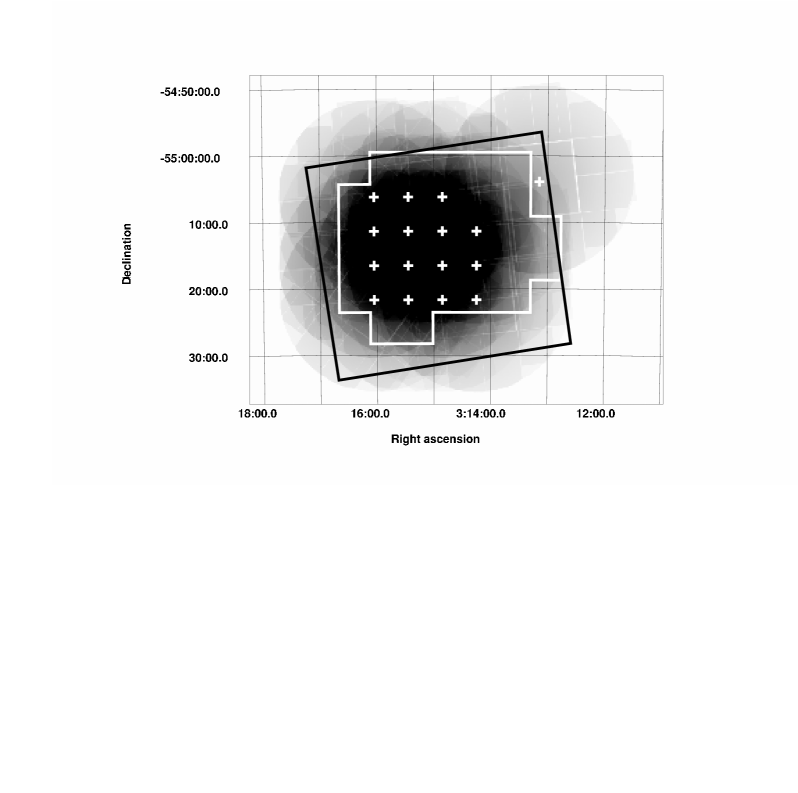
Figure 1: Averaged mos1 and mos2 exposure map (0.5-2.0 keV) of the $4\times 4$ pointing pattern (small white crosses). The exposure time in the central region reaches 78 ksec. The black rectangle shows the area covered by the WFI $R$-band images. The white polygon marks the area covered by the SOFI $K$-band images (see Sect. 2.2).

We then added the images, exposure maps, and background maps of the individual pointings, resulting in 15 images for 5 energy bands and 3 detectors. These images were used simultaneously as input for a detection run with eboxdetect and emldetect. The task emldetect applies a PSF-fit to each source found by eboxdetect in order to determine the source parameters. Since we use merged mosaic images of the field, each source image results from the superposition of several pointings. In each pointing the source is detected at a different position on the detector. Therefore, the standard configuration of emldetect, which uses the off-axis angle and position-angle of each source to extract the appropriate PSF from calibration files, could not be used here. Instead emldetect was modified to use the calibration PSF corresponding to an off-axis angle $\theta=5\,\rm{arcmin}$ throughout the entire field. This PSF is circular symmetric and is a good representation of the point sources in the merged images. For this work no extent models were fitted to the sources, therefore the source list produced by emldetect does not contain any information whether a source is extended or point-like. Generally, the X-ray data reduction and analysis was performed with XMM SAS version 5.1 (from 18/06/2001) with the abovementioned exception of an adapted version of emldetect. The version of emldetect used here suffered from an error, which resulted in the overestimation of detection likelihood values (XMM-Newton-NEWS #29, 11-Mar-2003). All likelihood values quoted here have been corrected to adhere to the relation $ML=-ln(P)$, where $ML$ is the detection likelihood and $P$ is the probability that the detection is caused by a random fluctuation of the background.

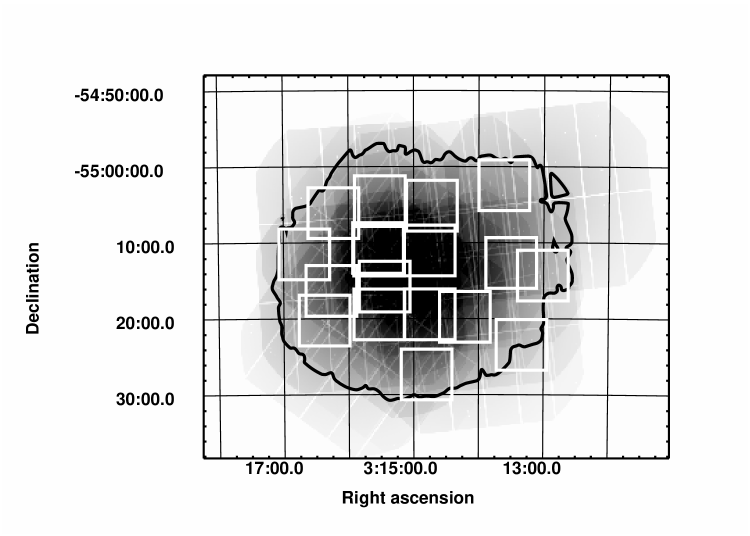
Figure 2: PN exposure map (0.5-2.0 keV) of the $4\times 4$ pointing pattern. The exposure time in the central region reaches 35.5 ksec. The area inside the black contour markes the ’core sample’ region where the pn-detector exposure time exceeds six ksec. White rectangles show the position of the spectroscopic masks for the optical follow-up observations (see Sect. 2.4).

All count rates and derived quantities are taken from the PSF fitting of emldetect. Using the combined expoure maps, emldetect corrects the source count rates for all spatial variations of telescope and detector efficiency, i.e. the count rates relate to the optical axis of each EPIC camera. Following Cash (1979) the 68% confidence intervals for the source positions and source fluxes were calculated using emldetect as follows: Each parameter is varied until the statistic

$C=2\sum\limits_{i=1}^{N}(e_{i}-n_{i}\ln e_{i})$

exceeds the best fit value of $C$ by 1, where $e_{i}$ is the source model at the position of pixel $i$ and $n_{i}$ is the number of counts in pixel $i$.

We used energy conversion factors (ECFs) to calculate source fluxes in the band 0.2-10 keV (from the total EPIC count rate in the band 0.2-12 keV) and in the band 0.5-2.0 keV (from the EPIC count rate in the band 0.5-2.0 keV). The ECFs were derived by using XSPEC and the XMM SAS calibration files to simulate power law spectra with photon index $\Gamma=1.8$ and the galactic column density of the field $N_{\rm H}=2.7\times 10^{20}\,{\rm cm^{-2}}$.

For all sources 3 hardness ratios of the form $HR=(CR_{2}-CR_{1})/(CR_{1}+CR_{2})$ were calculated between the adjacent pn-detector energy bands 0.2-0.5 keV, 0.5-2.0 keV, 2.0-4.5 keV, 4.5-7.5 keV. For example $HR2$ was calculated between the bands 0.5-2.0 keV and 2.0-4.5 keV. The different energy response of the mos- and pn-detectors result in different hardness ratios for the same source. If not noted otherwise the pn-values are used throughout the paper.

In total we detected 328 X-ray sources with detection likelihoods $ML\geq 5.0$. The X-ray fluxes are in the range $f_{\rm{X}}=(0.16-54)\times 10^{-14}$ erg cm^-2 s^-1 (0.2-10 keV). The X-ray flux histogram (Fig. 3) shows the X-ray detection limit of our survey. Below $f_{\rm{X}}\sim 5\times 10^{-15}$ erg cm^-2 s^-1 we are unable to detect the majority of the X-ray sources.

In the central region (Fig. 2) we found 252 X-ray sources. The complete X-ray source list can be found in the Online Material, Appendix A.

Since the PSF-modelling task emldetect was only used with point source models here, the detection procedure was not very sensitive to diffuse emission from clusters of galaxies. However, visual inspection of the X-ray images revealed no obviously extended sources.

We estimate that extended cluster emission down to 0.5-2.0 keV fluxes of $2\times 10^{-14}{\rm\,erg\,cm^{-2}\,s^{-1}}$ should be detectable in this survey. The cluster log$\,N$(log$\,S)$ of Rosati et al. (1998) gives a surface density of $\sim$6 clusters per square degree at this flux. We would therefore expect about 4 clusters in the total area of the XMM observations and about 2 clusters in the 0.28 deg² core region of the survey. Given the considerable cosmic variance of the cluster surface density the non-detection of clusters in the survey is consistent with the log$\,N$(log$\,S)$. In any case the small number of expected clusters does not suggest a significant contribution of clusters of galaxies to our source sample.

XMM-Newton redetected all 50 ROSAT X-ray sources (Zamorani et al. 1999). However, two ROSAT X-ray sources have low detection likelihoods and were thus not included in the final XMM-Newton X-ray source list (Online Material, Appendix A). Fig. 4 compares ROSAT and EPIC X-ray fluxes in the 0.5-2.0 keV band.

Figure 3: 0.2-10 keV X-ray flux histogram of the 328 XMM-Newton detected X-ray sources in the Marano Field. Up to an X-ray flux of $f_{\rm{X}}\sim 5\times 10^{-15}$ erg cm^-2 s^-1 (turnover flux) we detect more and more sources. Below that X-ray flux the detection rate decreases dramactically.

Figure 4: Comparison between the 0.5-2 keV X-ray fluxes measured by ROSAT and XMM-Newton of all 50 ROSAT X-ray sources in the Marano Field. XMM-Newton fluxes are averages of the three individual EPIC camera fluxes. The black solid line represents equal ROSAT and XMM-Newton fluxes.

The X-ray fluxes of both missions are comparable down to ROSAT fluxes of $f_{\rm{X}}\sim 6.0\times 10^{-15}$ erg cm^-2 s^-1. Among the 13 objects (broad emission line objects) with $f_{\rm{X}}\geq 10^{-14}$ erg cm^-2 s^-1 (ROSAT) five show variability of about a factor of two in both directions.

Throughout the whole paper we refer to the X-ray sources by mentioning the X-ray source number without any letter as suffix (e.g. 452). These numbers refer to the sequence numbers in the original emldetect source list and are non-contiguous due to the removal of sources below $ML=5.0$ after correction of the detection likelihoods.

2.2 The optical data

2.2.1 WFI $R$-band observations

The central region of the Marano Field has been observed in the $UBVRI$ bands with the ESO Wide-Field-Imager (WFI). Here we make use of the deep (7000 sec) $R$-band image (Mignoli & Zamorani 1998) with a limiting magnitude $R\simeq 22.5$ (defined as turnover magnitude minus 0.5 mag, see Fig. 5). The WFI-image covers an area of 35 $\times$ 32 arcmin well aligned with the region of the deepest XMM-Newton coverage (Fig. 1).

Figure 5: Magnitude histogram of the sources detected in the WFI $R$-band image. Completeness in detecting objects is lost for $R>23$.

2.2.2 SOFI $K$-band observations

The $K$-band data ($2.0-2.3\,\mu$m) were obtained at the ESO New Technology Telescope (NTT) with the SOFI instrument. With an area of 754 arcmin² the $K$-band mosaic covers a slightly smaller area than the WFI $R$-band observation and is well aligned with the deepest XMM-Newton exposure (Fig. 1). The SOFI observations consist of a mosaic of 33 jittered pointings, each covering $5\times 5$ arcmin with an exposure time of 29 minutes each. The limiting magnitude is $K\simeq 20$ (turnover magnitude minus 0.5 mag, see Fig. 6).

Figure 6: Histogram of the $K$-band magnitudes in the NTT-SOFI images. Completeness in detecting objects is lost for $K>20.5$.

2.2.3 VLT $R$-band pre-images

$R$-band pre-images for the spectroscopic follow-up observation were obtained with the Focal Reducer and Spectrograph FORS1 and FORS2 at the ESO Very Large Telescope (VLT). The first run (FORS1) contained six and the second run (FORS2) 12 optical images. The summed pre-imaging area is $\sim$530 arcmin² in the central region of the Marano Field (Fig. 2). Since the field was not contiguously covered by FORS spectroscopy, also the pre-images cover only $\sim$50% of the central area of the X-ray survey.

2.3 Target selection for optical spectroscopy

Our target selection for the optical spectroscopy was primarily based on FORS1/FORS2 $R$-band pre-images. WFI $R$-band and SOFI $K$-band data were used in addition to support the target selection on the pre-images in case of faint counterparts. The chosen fields represent a compromise in terms of maximum survey area and source density because of limited telescope time. First priority for spectroscopic follow up was given to candidates with a likelihood of existence $ML>10$ within a 2$\sigma_{\rm{X}}$ error radius. The total position error is $\sigma_{\rm{X}}=\sqrt{\sigma_{\rm{stat.}}^{2}+\sigma_{\rm{syst.}}^{2}}$. The statistical errors $\sigma_{\rm{stat.}}$ of the positions were calculated as described in Sect. 2.1. The systematic errors are caused by uncertainties in the spacecraft attitude, errors in the linearisation of the detector coordinates, and undersampling of the PSF (in particular for the PN camera). At this stage, we allowed a systematic position error of 2 arcsec, see Sect. 3.2 for a more accurate estimation of the systematic position errors.

The multi-object spectroscopy masks were designed with the software fims 2 provided by ESO. For all spectroscopic targets we used straight slitlets with a nominal length of ten arcseconds and width of one arcsecond. For extended sources or closely spaced candidate counterparts a different slit length, 6 – 14 arcseconds, was used. Still available mask positions were filled with candidate objects not fulfilling the main selection criteria and with additional random non X-ray emitting galaxies.

2.4 Spectroscopic observations

The FORS1 multi object spectroscopy (MOS) run with six masks was obtained on November, 20th in 2000 by using grism GRIS_150I+17. No order separation filter was used. The exposure time for every mask was 2400 seconds. The seeing was 0.7$\pm$0.1 arcsec.

The second run was performed with FORS2 in spectroscopic mask mode (MXU) from November, 27th-30th in 2002. We aimed for an exposure time of 3 $\times$ 1800 seconds per mask, but weather and time constraints required some deviations from this general scheme (Table 2). Grism GRIS_150I+27 was used for all masks.

Table 2: Details of FORS2 spectroscopic mask mode observation (see Fig. 2)

mask	observation	filter	seeing
	(each 1800s)		(in arcsec)
mask1	3	none	0.63
mask2	4	none	1.36
mask3	3	none	1.05
mask4	3	none	0.78
mask5	3	none	0.93
mask6	3	GC375	0.75
mask7	3	none	0.80
mask8	3	none	0.81
mask9	2	none	0.66
mask10	3	none	0.76
mask11	1	none	0.96
mask12	2	none	0.64

In order to prevent second order contamination, the first mask (mask6) in the observing sequence was observed through filter GC375 which limited the wavelength range from 3850 to 7500 Å. A comparison with the second mask without order separating filter showed that the contamination effect is negligible. Hence, for all following masks the filter was removed from the light path resulting in a wavelength range for central targets of the final spectra from 3500 to 10000 Å.

2.5 Spectroscopic data reduction

The reduction of the data was accomplished by a semiautomatic pipeline coded in MIDAS. It was specially designed to reduce FORS2-MXU data with as little interaction by the user as possible. After modifications this code was also used to reduce the FORS1-MOS data.
The bias correction was done in the standard manner with careful attention to possible time dependence on the bias level and dark current. An ordinary flat field correction was used to rectify the pixel-to-pixel variation.

2.5.1 Wavelength calibration

We established a 2-d wavelength calibration in the pipeline. This allowed to correct the distortion perpendicular to the dispersion direction and improved significantly the signal-to-noise ratio of the extracted spectra. The calibrated wavelength range is 3500–10000 $\AA$. However, many spectra were located close to the edge of the CCD. Hence, there are substantial variations in the wavelength range of the spectra. The average uncertainty of the wavelength calibration is 0.2 Å  but reaches a maximum of $\Delta\lambda\pm 1.5\,\AA$ at long and short wavelength ends. Further details on the

Table 3: Setups for the optical spectroscopy

	FORS1	FORS2
grism	GRIS_150I+17	GRIS_150I+27
dispersion [$\AA/$mm]	230	225
pixel size [$\mu$m]	24 x 24	15 x 15
step width [$\AA/$Pixel]	5	3

optical setups can be found in Table 3. We estimate the spectral resolution finally achieved by measuring the width of the arc lines in the lamp spectra to $\Delta\lambda\sim 21\AA$ (FWHM).

2.5.2 Object and sky definition

The aquisition slit-through images were used to roughly define the position and width of every single slit in an image. For an optimal definition of the object and sky region in the spectrum the pipeline then displays intensity profiles in graphic windows and an image of the corresponding spectrum. After a careful inspection of these pipeline outputs, the object and the sky region were defined manually for every single spectrum. Consequently, bad pixel/lines/colums in the raw data can be excluded for the extraction and scientific misinterpretation of artifacts in the final spectra can be avoided. Whenever possible, two sky regions, on both sides of the target spectrum, were defined.

2.5.3 Extraction of spectra

The extraction is based on an optimal extraction algorithm (Horne 1986) including a cosmic ray rejection. Extensive tests determined the optimal extraction parameters. Standard flux calibration was applied. Since FORS2-mask6 was observed with an additional filter, a different standard star was used. All spectra were corrected for atmospheric absorption using the standard ESO extinction correction function scaled to the given airmass.

The $n$ individual spectra of a given counterpart object were combined to form one single final spectrum. The individual spectra were firstly normalized to the same mean intensity. The normalization factor was determined from an analysis of all spectra in a given mask. The final spectrum is the uncertainty-weighted mean spectrum.

3 Spectroscopic classification of the X-ray counterparts

The spectroscopic classification of the individual X-ray sources was primarily based on the FORS1 and FORS2 spectra. In addition, we used optical and X-ray images for a reliable identification (see Online Material, Appendix C). Broad emission line objects were immediately accepted as X-ray counterparts. Narrow emission line galaxies and normal galaxies were accepted as X-ray counterparts, if no other optical candidate was found within the position error range. Stars were regarded as likely counterparts if the X-ray colors indicated a soft X-ray spectrum compatible with coronal emission of $\leq 1$ keV. Every X-ray identification was confirmed by at least two individuals.

For the large majority of our spectra the signal to noise ratio (SNR) is sufficient to give reliable classifications and redshifts. Like other X-ray identification surveys, we encounter the problem of difficult classification of the optical spectra below a certain SNR. For spectra with a SNR=3-5, the identification of narrow emission lines was still possible. However, at this SNR faint broad emission lines and normal galaxy spectra are very difficult to identify. Fig. 7 shows a spectrum of a narrow emission line galaxy with a SNR=2.4 (continuum near the O ii emission line), which is close to the identification limit. Only one significant narrow emission line at $\sim$7100 Å is found. The spectral shape makes it reasonable to identify this line as O ii emission line. Even though this classification is likely, an unambiguous redshift determination and classification of the type cannot be given. Spectra with a SNR less then $\sim$2.5 are not identifiable.

The reliability of the redshift determination and classification of the optical spectra is given by flags in column (9) flags of Table The XMM-Newton Survey in the Marano Field.

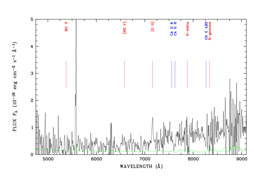
Figure 7: Optical atmospheric absorption corrected, wavelength and flux calibrated spectrum for X-ray source 480. The black spectrum marks the object’s spectrum. The green line (see the color online version of the manuscript) shows the error spectrum. Possible emission and absorption features in the spectrum are labeled. The spectral feature at 5580 Å is spurious due to incomplete substraction of a night sky line.

The complete list of X-ray classification is given in Table The XMM-Newton Survey in the Marano Field. The columns are described as follows:

(1) No
Classification of a counterpart object consists of the sequence number of the X-ray source list and a suffix (A, B) in order to discriminate between different candidates.

(2) RA [hh:min:ss] and (3) DEC [deg:min:ss]
Right ascension and declination of the optical candidate counterpart (J2000).

(4) dist_OX [arcsec]
Spatial offset between the X-ray and optical positions.

(5) K
SOFI $K$-band magnitude of the spectroscopically classified candidate, whenever available.

(6) R
WFI $R$-band magnitude of the spectroscopically classified candidate, whenever possible.

(7) class
Spectroscopic classification of the identified object. S – star, G – normal galaxy (no emission lines), N – narrow emission line galaxy with unresolved emission lines (at 6000 $\AA$ our spectral resolution of 21 $\AA$ corresponds to 1050 km/s), B – broad emission line object (all measured line widths have $v_{\rm{FWHM}}>2500$ km/s), ? – undefined object.

(8) $z$
Spectroscopic redshift of the identified object. The redshift is taken from the literature for objects with ’1 - -’ and ’0 - -’ in column ’(9) flags’. Column ’(15) remarks’ states the source of redshift determination and classification.

(9) $flags$
X-ray identification flag, redshift flag, and classification reliability flag. The first number (0,1) marks whether a spectroscopically classified object was accepted as X-ray counterpart. Objects which we consider to be the correct identification of the X-ray source are flagged by ’1’, while ’0’ flags objects not considered as the X-ray source.
The second (middle) flag states the redshift reliablility. A redshift flag ’1’ means a reliable, well established redshift determined by several spectral features. ’0’ marks objects where the redshift determination relies on a single but reasonable spectral feature.
The third (last) flag characterizes the classification reliability. A flag ’1’ marks that the object type as given in ’(7) class’ is well established and reliable. Flag ’0’ indicates an uncertain classification of the object type. Either high SNR spectral features of the object do not allow a proper classification or the optical spectra do not allow to give a reliable classification of the object type because of a low SNR and/or insufficient wavelength coverage of the optical spectra. The latter is illustrated in Fig. 7. The narrow O ii line indicates a narrow emission line galaxy. However, the SNR of the spectrum does not allow to judge the existence of a broad Mg ii line and, hence, a classification as type I AGN. Since C iv and C iii are outside the spectrum’s wavelength range, Mg ii is the only possible broad line feature. The most likely classification of this object is a narrow emission line galaxy. However, the given arguments show that a classification as type I AGN cannot be excluded. Therefore, the classification flag for this object is ’0’.
Objects with ’1 - -’ and ’0 - -’ have only an X-ray identification flag since their redshift and classification relies on follow-up surveys previously done in the Marano Field (see column ’(15) rem.’).

(10) log (L${}_{X_{OBS}}$ [erg s^-1])
Observed rest-frame X-ray luminosity (logarithmic units) in the 0.2-10 keV energy band calculated by using Eq. 1. The $k$-correction vanishes since we assume an energy index $\alpha=-1$ with $F_{\rm{\nu}}\sim\nu^{\,\alpha}\sim\nu^{\,1-\Gamma}$ ($\Gamma$ - photon index) based on Alexander et al. (2003) and Mainieri et al. (2002). The luminosity distance $d_{\rm{L}}$ was computed by the analytical fit for flat comologies with $\Omega_{\rm{m}}=0.3$, $\Omega_{\Lambda}=0.7$, $H_{\rm{0}}=70$ km s^-1 Mpc^-1 following Szokoly et al. (2004).

$$L_{\rm{X}}=\frac{4\,\pi\,d_{\rm{L}}^{2}}{(z+1)^{\,\alpha+1}}f_{\rm{X}}$$ (1)

(11) $M_{B}$
Absolute magnitudes $M_{\rm{B}}$ (in the Johnson system) were estimated only for type I AGN using the relation

$$M_{\rm{B}}=R+5-5\log(d_{\rm{L}}/\mathrm{pc})+K(z)$$ (2)

where $d_{\rm{L}}$ is the luminosity distance and $K(z)$ is the customary $k$-correction term.

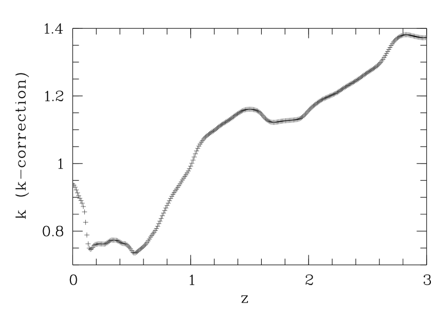
Figure 8: Adopted mean k correction from observed R-band to rest-frame $M_{\rm{B}}$, for broad emission line AGN.

In our case, this term includes the transition from observed-frame $R$-band to rest-frame $B$-band, assuming a mean spectral energy distribution for all sources, and also the $(1+z)$ bandwidth stretching factor. For the type I AGN we computed $K(z)$ from the composite SDSS quasar spectrum (Vanden Berk et al. 2001). The resulting graph is shown in Fig. 8.

(12) $\alpha_{OX}$
The broad band spectral index $\alpha_{\mathrm{OX}}$ roughly characterizes the UV–X-ray spectral energy distribution by connecting the rest-frame points at 2500 Å and 1 keV with a simple power law, $F_{\nu}\propto\nu^{-\alpha_{\mathrm{OX}}}$. For each broad emission line AGN we estimated its flux at a fixed rest-frame wavelength of $\lambda=2500$ Å, applying the relation

$$m_{\mathrm{AB}}(2500\,\mathrm{\AA})=R+\Delta m(z)$$ (3)

where $R$ is the quoted $R$-band magnitude, $m_{\mathrm{AB}}(2500\,\mathrm{\AA})$ is the predicted magnitude at 2500 Å – expressed in the AB system for easy conversion into monochromatic fluxes –, and $\Delta m(z)$ is a redshift-dependent term (similar, but not identical to the $k$-correction) that also accounts for the zeropoint transformation from the Vega to the AB system. Our adopted $\Delta m(z)$ relation, again computed from the SDSS composite quasar spectrum of Vanden Berk et al. (2001), is shown in Fig. 9. Notice that at the typical redshifts of $z\sim 1.5$ of our broad line AGN, the observed $R$-band approximately traces a rest-frame wavelength of $\lambda_{\mathrm{rest}}\sim 2600$ Å, implying that the spectral energy distribution corrections are small. The resulting AB magnitudes are then converted into fluxes following the definition of the AB system (Oke & Gunn 1983):

$$m_{\mathrm{AB}}(2500\,\mathrm{\AA})=-2.5\log(F_{\nu}(2500\,\mathrm{\AA}))-48.60$$ (4)

where $F_{\nu}(2500\,\mathrm{\AA})$ is given in erg s^-1 cm^-2 Hz^-1.

The X-ray flux at 1 keV is computed by:

$$f(0.2-10\,\mathrm{keV})=F_{\nu}(1\,\mathrm{keV})\int\limits_{0.2\,\mathrm{keV}}^{10\,\mathrm{keV}}E^{\alpha}\mathrm{d}E\,\,\,\,\,\,\,\mathrm{with}\,\,\alpha=-1\,.$$ (5)

Hence, the broad band spectral index is obtained as

$$\alpha_{ox}=\frac{\log(F_{\nu}(2500\,\mathrm{\AA}))-\log(F_{\nu}(1\,\mathrm{keV}))}{\log(\nu(1\,\mathrm{keV}))-\log(\nu(2500\,\mathrm{\AA}))}.$$ (6)

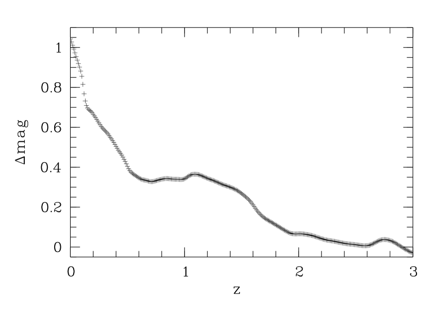
Figure 9: Adopted conversion term to estimate AB magnitudes at fixed rest-frame wavelength $\lambda=2500$ Å from observed R-band magnitudes.

(13) N_H [cm^-2]
X-ray absorbing hydrogen column density in units of $10^{22}\leavevmode\nobreak\ \mathrm{cm^{-2}}$ (see Sect. 4.4).

(14) log ($L_{X_{INT}}$ [erg s^-1] )
Intrinsic rest-frame X-ray luminosity (logarithmic units) in the 0.2-10 keV energy band after X-ray flux correction for the absorbing hydrogen column density. Calculation uses Eq. 1.

(15) rem.
Remarks for individual objects: 1 – optically selected and spectroscopically classified quasar by Marano et al. (1988), 2 – optically selected and spectroscopically classified quasar by Zitelli et al. (1992), 3 – ROSAT X-ray source with spectroscopic classification and redshift determination by Zamorani et al. (1999), 4 – ROSAT X-ray source with no or wrong identification by Zamorani et al. (1999), 5 – unclassified radio objects within 5 arcsec, Gruppioni et al. (1999), 6 – spectroscopic classification and redshift taken from Teplitz et al. (2003), 7 – radio source, spectroscopic classification and redshift taken from Gruppioni et al. (1999), C – individual comment to an object (see 3.1).

3.1 Comments to individual objects

9A: New redshift determined for this source, formerly known as Zamorani et al. (1999) X043-12.

15A: Object 15A is not regarded as the optical counterpart, since the identification of the line features is uncertain and the positional offset is rather large. A very faint object at the detection limit lies in the X-ray error circle. A lower limit of $f_{\rm{X}}/f_{\rm{opt}}\sim 65$ for this source was estimated by assuming a limiting magnitude of $R=24$.

17A: Source 17 is a likely X-ray blend with large contrast between the two individual sources. Object 17A is a unique identification of the brighter X-ray source, whose X-ray flux is likely to be overestimated due to blending.

20A & 20B: Zamorani et al. (1999) identified source 20 with the M-star 20B. Some contribution of the M-star’s X-ray flux cannot be excluded, but the identification with the type II AGN (object 20A) seems more likely, since the X-ray colors indicate a relatively hard spectrum.

22A & 22B: X-ray source 22 is a probable blend. Objects 22A and 22B fall on top of the two suspected point sources. We regard both optical objects as likely counterparts of the X-ray blend and distribute the measured X-ray flux evenly between the two sources.

26A: New redshift determined for this source, formerly known as Zamorani et al. (1999) X301-29.

32A: NV strongest emission line in the spectrum (brighter than Ly-$\alpha$). Narrow emission lines are present and the object is classified as ’N’ (narrow emission line galaxy). However, all narrow emission lines have underlying broad components. Therefore, the classification flag is set ’0’.

35A & 35B: Two galaxies at equal redshift, the brighter galaxy 35A is regarded as the X-ray counterpart. A nature of the X-ray source as galaxy cluster cannot be completely excluded but an X-ray extent is not obvious. For 35A a new redshift is determined (update to Zamorani et al. (1999) X022-48).

42A: New redshift determined for this source, formerly known as Zamorani et al. (1999) X031-24.

46A: X-ray blend with major contribution from the southwestern component with type I AGN 46A as counterpart.

47A & 47B: Two narrow emission line galaxies at equal redshift. A nature of the X-ray source as galaxy cluster cannot be completely excluded, but an X-ray extent is not obvious. 47A is assumed as optical counterpart.

63A: Unresolved narrow emission lines are present and the object is classified as ’N’ (narrow emission line galaxy). However, the C iv emission line has an underlying broad component. Therefore, the classification flag is set ’0’.

66A: The identification is not unique, since the optical image reveals a possible second object inside the 1$\sigma$-X-ray position error circle.

133A: Narrow emission lines are present. The object is classified as ’N’ (narrow emission line galaxy). However, Ly-$\alpha$ shows a resolved, broad base. Therefore, the classification flag is set ’0’.

151A: Probably a spurious detection of the X-ray source. The source is kept in the source list for the formal reason of having an $ML=5.2$ but is not considered further.

191A: Optical spectrum in Zitelli et al. (1992) indicates a type I AGN with typical broad emission lines. However, this object shows the lowest X-ray to optical flux ratio of all AGN in our sample. $f_{\rm{X}}/f_{\rm{opt}}=0.04$ suggests an X-ray faint AGN. Since this object was not detected by ROSAT, it is unlikely that the extreme $f_{\rm{X}}/f_{\rm{opt}}$-ratio is due to a temporary low X-ray state of the object. Furthermore, it is one of the type I objects with intrinsic absorption ($N_{\rm{H}}=(5.75_{-2.81}^{+3.83})\times 10^{22}\,{\rm{cm}}^{-2}$).

217A & 217B: X-ray blend, the identification of 217A with the southeastern component seems unambiguous, the identification of 217B with the northwestern component is not unique, since a similarly bright, close-by, but still unidentified object is present at the same distance from the X-ray source.

224A & 224B: Two galaxies at equal redshift, no obvious X-ray extent.

253A & 253B: Two objects at similar redshift with $2\,\mathrm{mag}$ difference in the optical. The brighter object 253A is regarded as the identification.

280A: Object is classified as ’B’ since C iii is well resolved with $\Delta\lambda\sim 72\AA$ (FWHM). Ly-$\alpha$ and C iv are narrow emision lines, but show strong absorption with broad underlying components. The classification flag is set ’0’. Possible broad absorption line quasar.

361A: Broad absorption line quasar.

382A & 496A: Physical quasar pair, separated by $17\arcsec$, at $z=1.904$, d_A = 143 kpc. The spectra are different, i.e. the two objects are not lensed images of the same source.

437A: Spectrum, optical and X-ray image, and relative soft hardness ratios point undoubtedly to an M-star as X-ray source. However, a flux ratio $f_{\rm{X}}/f_{\rm{opt}}=1.7$ is unusually high for an M-star as the X-ray identification.

512A & 512B: Zamorani et al. (1999) identify the NELG 512B with the X-ray source. The $2\,\mathrm{mag}$ fainter NELG 512A lies somewhat closer to the X-ray position. While both galaxies may contribute to the observed X-ray flux, we assume object 512A as the counterpart in the following.

582A: Spectrum, optical and X-ray image, and relative soft hardness ratios point undoubtedly to an M-star as X-ray source. However, a flux ratio $f_{\rm{X}}/f_{\rm{opt}}=1.5$ is unusually high for an M-star as the X-ray identification.

607A & 653: Detected as a single X-ray source by ROSAT Zamorani et al. (1999) X404-23, X-ray source 653 is brighter and closer to X404-23 and, therefore, treated as the detected ROSAT X-ray source. The broad spectral feature at 7100$\,\AA$ in the optical spectrum of 607A is spurious due to the zeroth order light of the neighbouring slit.

615A & 615B: Both objects, the broad emission line object 615A and the narrow emission line object 615B, are possible counterparts to the X-ray source. We regard the fainter, but positionally better matching object 615A as the counterpart.

632A: Spectrum suggests a BL-Lac object, but the object is not a radio source, classification unclear.

3.2 Discussion of spurious matches

Since type I AGN are a well-established class of X-ray emitters with relatively low surface density, false matches should not play any role for this object class.

However, when investigating the classes of optically normal and narrow emission line galaxies, the problem of false matches has to be taken into account due to the high surface densities of these objects. In order to check the quality of our optical X-ray counterpart identification, we applied various tests.

First, the derived false match rate will depend on the assumed position errors which takes into account the statistical and the systematic position error (see Sect. 2.3). The difference in X-ray and optical position scaled to a 1$\sigma_{\rm{X}}$ position error is shown in Fig. 10 a. When we assume systematic errors of 2 arcsec, the theoretical Gaussian distribution (Eq. 7)

$$f(r_{\rm{n}})=N_{\rm{tot}}\,r_{\rm{n}}e^{-\frac{1}{2}r_{\rm{n}}^{2}}\,\,,\,\,r_{\rm{n}}=\frac{r_{\rm{X}}-r_{\rm{O}}}{\sigma_{\rm{X}}}$$ (7)

peaks significantly later than the observed distribution of the X-ray counterparts. This is not due to the fact that we systematically accepted spurious counterparts sources, since the type I AGN distribution (shown with dotted lines in Fig. 10) is consistent with the total X-ray identification distribution. The fact that we have a large number of type I AGN allows to estimate the actual systematic position error for our X-ray observation. The observed distribution of the type I AGN position errors can be well reproduced with a systematic error

Figure 10: a) Number of objects identified as X-ray counterparts vs. difference in X-ray and optical position scaled to a 1$\sigma_{\rm{X}}$ position error with a systematic X-ray position error of 2 arcsec. The smooth line represents the theoretical distribution. The distribution of type I AGN, which are a class of well-accepted X-ray emitters, is plotted as a dotted line. The solid line characterizes the complete sample including type I AGN, type II AGN, galaxies, and stars; b) The 1$\sigma_{\rm{X}}$ position error was adjusted to the observed distribution by reducing the systematic X-ray position error from $2\arcsec$ to $0.7\arcsec$. The complete sample agrees well with the type I AGN distribution which gives evidences of a marginally false match rate.

of $\sigma_{\rm{syst.}}=0.7\arcsec$ (Fig. 10 b). Moreover, the distribution of normalized position differences for the total sample agrees well with the theoretical distribution and with the type I AGN distribution when we apply $\sigma_{\rm{syst.}}=0.7\arcsec$.

Considering $\sigma_{\rm{syst.}}=0.7\arcsec$, we calculate the false match rate by following Sutherland & Saunders (1992) and Ciliegi et al. (2003). For every spectroscopically classified counterpart we determine the likelihood ratio $L$ by

$$L=\frac{Q\,exp(-dist_{\rm{OX}}^{2}/2)}{2\pi\sigma_{\rm{X}}^{2}N(<m_{\rm{R}})}$$ (8)

where L is the probability of finding the true optical counterpart in this position with this magnitude, relative to that of finding a similar chance background object. Hence, the reliability of a counterpart is given by $P_{\rm true}=L/(1+L)$. $Q$ is the probability that the counterpart of the X-ray source is brighter than the limit of the optical survey and has here been set to $Q=0.5$. $N(<m_{\rm{R}})$ is the number density of catalogue objects of the relevant class brighter than the counterpart. For narrow emission line counterparts we assumed that about one third of the field galaxies show line emission detectable in our spectra (Kennicutt 1992). We therefore derive the density of background objects $N(<m_{\rm{R}})$ by multiplying the total number of objects $<m_{\rm{R}}$ in the optical catalogue by a factor $0.33$. For normal galaxies a factor of $0.67$ was applied accordingly.

The total number of false matches can then be calculated by adding up all probabilities $P_{\rm sp}=1/(1+L)$ that the counterpart is spurious. Statistically, $\sim$25% of our normal and narrow emission line galaxy are spurious counterparts. However, after visually examining objects with low probabilities $P_{\rm true}$, we find that in at least two cases (422A, 485A) the X-ray position given by the source detection software is influenced by blending with another X-ray source and the counterparts are consistent with the peak of the brighter X-ray source (see Appendix C, finding chart). Taking this into account, we estimate that the false match rate is $\sim$20% for the sample of type II AGN. For the optically normal galaxies the false match rate calculated with the likelihood method is $\sim$2%.

As a further quality check we plot the position error vs. WFI $R$-band magnitude. False matches would be recognizable due to different distributions of the type I and type II counterparts in this diagram. However, Fig. 11 shows that all object classes occupy the same regions in the diagram. Hence, the diagram does not indicate any serious contamination by false matches even for faint counterparts.

Figure 11: WFI $R$-band magnitude vs. difference in X-ray and optical position scaled to a 1$\sigma_{\rm{X}}$ position error with a systematic X-ray position error of 0.7 arcsec. Crosses mark type I AGN, asterisks type II AGN, triangle galaxies, rectangles stars.

3.3 Classification summary

In total, we spectroscopically classified 140 of the optically identified X-ray sources. Details are shown in Table 4.

Table 4: Origin of optical counterparts to XMM sources

obtained optical spectra for X-ray sources	207
positive literature classifications by Marano
et al. (1988) and Zitelli et al. (1992) (partly reobserved)	30
new optical counterparts of ROSAT sources
Zamorani et al. (1999) (partly reobserved)	14
new positive spectroscopic classifications of XMM sources	96
total positive spectroscopic classifications of XMM sources	140

Like in other deep surveys, e.g. Hasinger et al. (2001), the majority of X-ray counterparts ($\sim$90%) is related to the accretion on supermassive black holes (type I and type II AGN). Furthermore, we classified a few galaxies and stars as optical counterparts (see Table 5).

Table 5: X-ray counterpart distribution

object class	total number	percentage
broad emission line objects (B)	89	63%
narrow emission line objects (N)	36	26%
galaxies (G)	6	4%
stars (S)	9	7%

4 Properties of a core sample of the XMM-Newton Marano survey

Our survey suffers somewhat from incomplete optical coverage of the X-ray survey area and, hence, a low identification rate over the whole area. In order to reach conclusions for the survey of a certain statistical significance we constrain our survey area and sample size to the central 0.28 deg² with a pn-exposure $>$6 ksec and significance of detection of individual sources with $ML>10$. We refer to this as the ’core sample’. See Fig. 2 for the definition of the core region. Note that the maximum exposure is 35.5 ksec for the PN camera and 78 ksec for each of the MOS cameras.

The core sample contains 170 X-ray sources ($ML>10$). No optical data are available for six out of the 170 X-ray sources which fall outside the WFI $R$-band image and are also not covered by VLT pre-images. Further six X-ray sources from the core sample have no optical detection in the WFI $R$-band image in a 3$\sigma_{\rm{X}}$ position error circle ($\sigma_{\rm{syst.}}=0.7\arcsec$). 122 X-ray sources are new detections, while 35 are spectroscopically classified ROSAT X-ray sources, and 13 are optically unidentified ROSAT sources. Out of the 140 spectroscopically classified objects in the Marano Field, 110 are associated to X-ray sources of the core sample. A summary of the properties of the core sample is given in Table 6.

Fig. 12 shows $R$-band magnitude histograms of the core sample X-ray sources that were spectroscopically classified and only optically identified respectively. The ($f_{\rm{X}}$,$ML$)-distribution of X-ray sources in the core region is given in Fig. 13.

The identification ratio of the core sample is 65%. In the next subsections we always refer to this sample.

Table 6: Properties of the core sample

X-ray sources ($t_{\rm{PN}}>6$ ksec, $ML>10)$		170
optically identified X-ray counterparts		158
spectroscopically classified optical counterparts		110

Figure 12: WFI $R$-band magnitude histogram for the core sample in the XMM-Newton Marano Field survey. The solid line represents the $R$-magnitude distribution of the spectroscopically classified X-ray counterparts. The dashed line shows the distribution of the optically identified but not spectroscopically classified X-ray counterparts. Six X-ray sources, which have no counterpart within a 3$\sigma_{\rm{X}}$ error circle, are assigned to the bin at $R$=25.0.

Figure 13: Likelihood vs. 0.2-10 keV X-ray-flux of the 252 central X-ray sources (pn-detector exposure time $\geq$6 ksec). Crosses mark type I AGN, asterisks type II AGN, triangle galaxies, rectangles stars. Dots indicate X-ray sources with no spectroscopic classification. The vertical line indicates $ML=10$.

4.1 X-ray properties

Characterising X-ray sources only by the X-ray properties can be used to reveal and study the existence of different X-ray populations and their features. Hardness ratios (see Sect. 2.1) are the simplest tool to determine the spectral energy distribution in the X-ray regime. In Fig. 14 ($HR2$ vs. $HR3$) we only plot those X-ray sources in an X-ray color-color diagram which have $HR2$ error $\sigma_{\rm{HR2}}\leq 0.3$. The different spectroscopically classified classes occupy different regions in this X-ray color-color diagram. A noticable separation in type I and type II AGN can be recognized. This result is in agreement with Mainieri et al. (2002) and Caccianiga et al. (2004). Type II AGN spread over a much broader $HR2$ ($0.9>HR2>-0.6$). The lowest $HR2$ values for type II AGN overlap with the highest $HR2$ values for type I AGN. However, we do not see a large fraction of type II AGN occupying the $HR2$ range typical for type I AGN, as was reported by Della Ceca et al. (2004) for the XMM-Newton bright serendipitous survey. Fig. 14 shows that $HR2$ is a good indicator for intrinsic absorption. The X-ray sources with $HR3=-1.0$ correspond to non-detections in the 4.5-7.5 keV band. The objects with $HR3>0.4$ and soft $HR2$ values have $HR3$ errors $\geq 0.3$ (small plot symbols). Therefore, it is likely that their deviation from the typical location of sources in the $HR2$ vs. $HR3$ diagram is caused by statistical fluctuations.

Figure 14: X-ray diagnostic diagram based on hardness ratios. $HR2$ is calculated by using the 0.5-2.0 keV & 2.0-4.5 keV band, $HR3$ 2.0-4.5 keV & 4.5-7.5 keV. Plotted are only X-ray sources that have $\sigma_{\rm{HR2}}<0.3$. Labels: crosses - 63 type I AGN, asterisks - 24 type II AGN, triangles - 4 galaxies, open circles - 24 unidentified X-ray sources with $ML>10$. Large symbols represent objects with $\sigma_{\rm{HR3}}<0.3$, small symbols $\sigma_{\rm{HR3}}\geq 0.3$. The solid line with box symbols (at $HR2\sim HR3\sim-0.5$) represents an unabsorbed powerlaw X-ray spectrum (corrected for galactic absorption) with different photon index $\Gamma=2.4-1.2$ in steps of 0.2 (squares). Different hydrogen column densities ($N_{\rm{H}}$/cm${}^{-2}=10^{20},10^{22},3\times 10^{22},10^{23},3\times 10^{23},10^{24}$; see Sect. 4.4) are plotted as a solid line with diamonds for $\Gamma=2$ and $z=1$.

The small number of optically normal galaxies span a large range in $HR2$. Two have $HR2$ values that belong to the softest in the whole core sample. The other two have X-ray spectra similar to those of soft type II AGN or very hard type I AGN.

In addition to the spectroscopically classified objects we plot also unidentified objects from the core region. Out of the total 60 unidentified X-ray sources, only 24 meet the selection criterion of $\sigma_{\rm{HR2}}\leq 0.3$. Based on the rather clear separation between type I and II AGN one may assign a likely classification to the yet unidentified sources. Among the 24 unidentified sources with reliable X-ray colors the numbers of type I and type II AGN candidates appear to be similar.

4.2 Redshift distribution

Figure 15: Redshift distribution of AGN in the Marano Field. a) complete sample of 64 optically selected quasars ($B_{\mathrm{J}}\leq 22.0$) by Zitelli et al. (1992); b) ROSAT X-ray sources (29 type I AGN by Zamorani et al. (1999)); c) 35 type I AGN newly detected by XMM-Newton (core region); d) Redshift distribution of the core sample. Dotted line: all 70 XMM-Newton detected type I AGN, solid line: 31 XMM-Newton detected type II AGN, dashed line: 5 XMM-Newton detected optically normal galaxies.

Previous extensive studies of AGN in the Marano Field enable us to compare these samples with our XMM-Newton detections. The optical survey by Zitelli et al. (1992) covers $\sim$0.7$\leavevmode\nobreak\ {\rm deg}^{2}$. The selected quasars, which are all of type I, show an almost flat distribution in redshift (Fig. 15 a) up to $z=2.8$. The ROSAT $0.2\leavevmode\nobreak\ {\rm deg}^{2}$ survey in the field (Zamorani et al. 1999) recovered most of the optically selected quasars at redshifts up to $z\sim 1.4$ (Fig. 15 b). The newly detected ROSAT AGN, with few exceptions, are type I AGN, which is expected due to the limited capability of ROSAT to detect absorbed sources.

In the $0.28\leavevmode\nobreak\ {\rm deg}^{2}$ core region of the XMM-survey we have detected 23 of the 29 broad emission line quasars of the optically selected sample of Zitelli et al. (1992). The detection rate of optically selected quasars remains constantly high over all redshifts.

However, looking at the type I AGN newly discovered with XMM-Newton, (Fig. 15 c) it is apparent that the X-ray selection tends to detect quasars at lower redshifts than the optical surveys. This is particularly obvious from the redshift distribution of the ROSAT detected quasars, representing the brightest X-ray sources in the field. But also the mean redshift $z\sim 1.3$ of the XMM-Newton detected type I AGN is lower than that of the optically selected sample $z\sim 1.5$, despite the fact that the XMM-Newton-observations are deeper in terms of the surface density of quasars than the optical survey. Possible reasons for these differences are discussed in Sect. 6.

The redshift distribution according to object class of the XMM-Newton detected core sample is given in Fig. 15 d. We find that almost half of the new XMM-Newton sources are classified as type II AGN with redshifts mostly below 1.0. Type I AGN extend over a wide range of redshifts with a maximum at $z\sim 0.8-1.4$. Type II AGN are comparable to type I AGN in number density at low redshifts, but are mostly found below $z=1$. Five type II quasars at $z>2.2$ have been identified. Optically normal galaxies without emission lines are found at $z<0.9$.

4.3 Observed X-ray luminosity

For the X-ray sources with measured redshifts X-ray luminosities can be computed. The coverage of the survey in redshift – X-ray luminosity space is plotted in Fig. 16. Szokoly et al. (2004) showed that the different object classes identified in X-ray surveys occupy different regions in a diagram of hardness ratios versus observed X-ray luminosities. In Fig. 17 we follow a scheme similar to that adopted by Szokoly et al. (2004) and consider objects with an X-ray luminosity log$(L_{\rm{X}})\geq 44.0$ as quasars (QSOs). The majority of type I AGN ($\sim$70 %) are actually type I QSOs. Most of type II AGN ($\sim$71 %) are low X-ray luminosity objects. Only type II objects with redshifts $z\geq 2.0$ (marked in grey in Fig. 17) have X-ray luminosities of type II QSOs.

Figure 16: Observed X-ray luminosity (0.2-10 keV) vs. redshift. Labels: crosses - 70 type I AGN, asterisks - 30 type II AGN, triangles - 5 galaxies.

Figure 17: Observed X-ray luminosity (0.2-10 keV) vs. hardness ratio. $HR2$ is calculated by using 0.5-2.0 keV & 2.0-4.5 keV bands. Plotted are only X-ray sources that have $\sigma_{\rm{HR2}}<0.3$. Labels: crosses - 63 type I AGN, asterisks - 24 type II AGN (grey marked have $z\geq 2.0$), triangles - 4 galaxies. The diagram separation into different regions is based on Szokoly et al. (2004) with an adjusted threshold in the $HR2$-value.

High-redshift type II QSOs with intrinsic absorption are found to be indistinguishable from non-absorbed type I AGN on the basis of their X-ray spectral hardness ratios, since the absorbed part of the spectrum is shifted out of the observable spectral window towards lower energies. This explains the emptiness of the upper right corner of Fig. 17 labeled ’Type II QSO’, a classification which applies to low redshift objects only.

Optically normal galaxies vary clearly in X-ray luminosity. The $HR2$-soft objects have very low X-ray luminosities. The two $HR2$-hard normal galaxies are found in the same region as the softest type II AGN, but are harder than type I AGN.

Szokoly et al. (2004) use $HR2=-0.2$ as a threshold for the separation of type I and type II objects. Assuming a $\Gamma=2$, this value corresponds to a hydrogen column density $N_{\rm{H}}$/cm${}^{-2}=10^{22},10^{23}$ for $z=0.25,2.1$, respectively. For their CHANDRA observation they computed $L_{\rm{X}}$ in the 0.5-10 keV band and their hardness ratio was based on the 0.5-2 keV & 2-10 keV bands. Because their definition of the X-ray bands differs from our study, the majority of their objects have higher hardness ratios (compared to our $HR2$). Furthermore, the XMM-Newton pn-detector, that was used for calculating the hardness ratios, has a higher efficiency in the 0.5-2 keV band compared to the CHANDRA detector. Therefore, we lowered the $HR2$ threshold from $HR2=-0.2$ in Szokoly et al. (2004) to $HR2=-0.45$. Our threshold corresponds to $N_{\rm{H}}$/cm${}^{-2}=0.54\times 10^{22},1.7\times 10^{22},5.4\times 10^{22}$ for $\Gamma=2$ and $z=0.25,1,2.1$. This is about two times lower than the $N_{\rm H}$ cutoff Szokoly et al. (2004) are using.

4.4 N_H column densities and corrected X-ray luminosities

The hardness ratio diagram (Fig. 14) supports the view that the majority of type II AGN and a small fraction of type I AGN are obscured sources. Hence, the observed X-ray luminosity does not represent the intrinsic object X-ray luminosity.

The significant deficit of soft photons as compared to a power law spectrum reflects the existence of an absorbing component that is expressed by the hydrogen column density $N_{\rm{H}}$. For most of the sources the number of detected counts is not sufficient to extract a spectrum and fit a power law model with $N_{\rm{H}}$ and the photon index $\Gamma$ as free parameters. We, therefore, applied a technique which uses the measured hardness ratios to calculate the $N_{\rm{H}}$ value for each source with a set of fixed power law indices. Mainieri et al. (2002) found a mean value of $<\Gamma>\simeq 2$ for 61 type I and type II AGN in the Lockman Hole. The majority of type I and II AGN are found in the range of $\Gamma\simeq 1.7-2.3$. The finding is confirmed by Mateos et al. (2005). They find $<\Gamma>=1.92$ with a $\sigma=0.28$. Therefore, we use the observed pn-, mos1-, and mos2-hardness-ratios (0.2-0.5 keV & 0.5-2.0 keV & 2.0-4.5 keV & 4.5-7.5 keV) and performed three runs to determine $N_{\rm{H}}$ with the values $\Gamma=1.7,2.0,2.3$ for all objects.

First of all, we computed a grid of model hardness ratios for all EPIC instruments with Xspec (using the models wabs, zwabs, and powerlaw). As input the galactic absorption in the line of sight in the field with $N_{\rm{H}}=2.7\times 10^{20}$ cm^-2, the redshift of the object and a grid of hydrogen column densities ($N_{\rm{H}}=0,\,N_{\rm{H}}=10^{20+0.04\,a}\ \mathrm{cm^{-2}},\ \ a\in N_{\rm{0}},\ \ a=0..100$) is used. We then computed the $\chi^{2}$ values for the deviations of the measured hardness ratios and their model values, summed over the three instruments and the three hardness ratios $HR1$, $HR2$, $HR3$. The procedure was applied only to those sources which had at least five out of nine hardness ratios with $\sigma HR_{\rm{obs,i}}<0.7$.

The $N_{\rm{H}}$ of a source is determined by finding the minimum of

$$\chi^{2}(N_{\rm{H}})=\sum_{i}\frac{(HR_{\rm{obs,i}}-HR_{\rm{model,i}}(N_{\rm{H}}))^{2}}{\sigma HR_{\rm{obs,i}}^{2}}\ \ .$$

The models are based on the photon index $\Gamma=2$.

The statistical 1$\sigma$ errors were derived from the range in $N_{\rm{H}}$, where $\chi^{2}<\chi^{2}_{\rm min}+1$ (Lampton et al. 1976). For the error calculation we also took into account an intrinsic scatter in the photon indices. Its contribution to the $N_{\rm{H}}$ error was measured by finding the minimum $\chi^{2}$ for each source in the grids calculated using $\Gamma=1.7$ and $\Gamma=2.3$. The resulting systematic errors were quadratically added to the statistical errors. The $N_{\rm{H}}$ values and the total errors are given in Table The XMM-Newton Survey in the Marano Field. Due to the uncertainties in the $N_{\rm{H}}$ determination we regard all values with $N_{\rm{H}}\leq 10^{21}\leavevmode\nobreak\ \mathrm{cm^{-2}}$ as consistent with unabsorbed spectra.

We tested our procedure by performing an individual Xspec $N_{\rm{H}}$-fit for the brightest type II AGN, which has sufficient X-ray data quality. The hardness ratios of 32A (z=2.727) indicate the highest absorption among the brightest type II AGN. A spectral fit with wabs, zwabs, powerlaw, and $\Gamma$ as a free parameter determined $N_{\rm{H_{32A}}}=(10.0\pm 3.5)\times 10^{22}\leavevmode\nobreak\ \mathrm{cm^{-2}}$ and $\Gamma_{\rm{32A}}=(1.7\pm 0.3$). The best fit $N_{\rm{H}}$, for a fixed value of $\Gamma=1.7$, with the hardness-ratio $\chi^{2}$-minimum fit is $N_{\rm{H_{32A}}}=(7.5\leavevmode\nobreak\ _{-2.8}^{+3.4})\times 10^{22}\leavevmode\nobreak\ \mathrm{cm^{-2}}$.

A spectral fit with a fixed $\Gamma_{\rm{32A}}=2.0$ results in $N_{\rm{H_{32A}}}=(13.4\pm 2.5)\times 10^{22}\leavevmode\nobreak\ \mathrm{cm^{-2}}$. The given $N_{\rm{H}}$ in Table The XMM-Newton Survey in the Marano Field was performed with the hardness-ratio $\chi^{2}$-minimum fit and finds $N_{\rm{H_{32A}}}=(14.5\leavevmode\nobreak\ _{-8.2}^{+7.9})\times 10^{22}\leavevmode\nobreak\ \mathrm{cm^{-2}}$. Hence, both fit methods give comparable results, at least for high SNR sources.

Fig. 18 shows the computed hydrogen column densities for type II AGN and optically normal galaxies.

Figure 18: Calculated intrinsic hydrogen column density histogram for the central Marano Field. The solid line shows the distribution of type II AGN that have reasonable fits in hydrogen column density. Objects with $N_{\rm{H}}=0$ are set to $N_{\rm{H}}=5\times 10^{19}\leavevmode\nobreak\ \mathrm{cm^{-2}}$. The dotted line represent only type II AGN that show intrinsic absorption with a significance higher than $2\sigma$ in hydrogen column density. Optically normal galaxies are plotted as a dashed line. Dotted line - 14 type I AGN; solid line - 30 type II AGN; dashed line - 5 galaxies.

As expected, the majority of type II AGN shows absorption. However, 13% of the type II objects (51A, 132A, 133A, 607A) have absorbing column densities $N_{\rm{H}}<10^{21}\leavevmode\nobreak\ \mathrm{cm}^{-2}$. All of the type II AGN discovered by Mainieri et al. (2002) in the Lockman Hole have absorbed X-ray spectra. The values for optically normal galaxies range from unabsorbed to moderately absorbed. Two of the unabsorbed galaxies have low X-ray luminosities ($L_{\rm X}<10^{42}\,{\rm erg\,s^{-1}}$).

The computed hydrogen column density of type II AGN object 145A is the highest in our sample ($N_{\rm{H}}=10^{24}\leavevmode\nobreak\ \mathrm{cm}^{-2}$). Since this corresponds to the highest value in the model grid, no reliable error estimate can be given for this object. However, the extremely high column density for this object is confirmed by the fact that it is one of the few sources detected in the $4.5-7.5\,{\rm keV}$ EPIC images, but it is not visible in the softer bands.

Based on the hydrogen column densities we calculated the unabsorbed (intrinsic) X-ray luminosities by computing a correction factor for the observed X-ray flux. Fig. 19 shows the comparison of the absorbed (a) and unabsorbed (b) X-ray luminosity distributions. Even after correcting the X-ray luminosity, type II AGN have lower median X-ray luminosities than type I AGN, although type I and II AGN cover the same X-ray luminosity range. In contrary to the almost flat distribution of type II AGN with a median of $L_{\rm{X}}\sim 10^{44}\,\mathrm{erg\leavevmode\nobreak\ s^{-1}}$, type I AGN show a significant peak at $L_{\rm{X}}\sim 10^{44.4}\,\mathrm{erg\leavevmode\nobreak\ s^{-1}}$ in observed and intrinsic X-ray luminosity. Type I AGN 5A exhibits the highest X-ray luminosity in our sample.

The hydrogen column density as a function of the intrinsic X-ray luminosity is shown in Fig. 19 c). Mainieri et al. (2002) suggest to label the region defined by $N_{\rm{H}}>10^{22}\leavevmode\nobreak\ \mathrm{cm}^{-2}$ and $L_{\rm{X}}>10^{44}\,\mathrm{erg\leavevmode\nobreak\ s^{-1}}$ as “type II QSO region”. They proposed this classification based on 61 AGN identified from XMM-Newton sources in the Lockman Hole. Following this classification our sample includes 10 type II QSOs.

In our case this region of the plot is also populated by nine type I QSOs, which formally have intrinsic hydrogen column densities $N_{\rm{H}}>10^{22}\leavevmode\nobreak\ \mathrm{cm}^{-2}$. However, most of these detections of intrinsic $N_{\rm{H}}$ have low significance, only four of all type I QSOs show absorption at the $2\sigma$ level (see Table LABEL:absorbed).

For about half of the type II AGN significant intrinsic absorption ($N_{\rm{H}}>2\times\Delta N_{\rm{H}}$) was measured, no dependence of the absorbed fraction on luminosity is evident (Table LABEL:absorbed).

Figure 19: a) Histogram of the absorbed (observed) X-ray luminosity (0.2-10 keV) for the core sample. Dotted line - 70 type I AGN, solid line - 30 type II AGN, dashed line - 5 galaxies; b) Histogram of the X-ray luminosity (0.2-10 keV) corrected for intrinsic absorption (core sample). Same notation as in a); c) Corrected X-ray luminosity (0.2-10 keV) vs. hydrogen column density (core sample). Crosses - type I AGN, asterisks - type II AGN, triangles - galaxies. The upper right corner is suggested to be defined as “Type II QSO region” by Mainieri et al. (2002). Objects with $N_{\rm{H}}=0$ are set to $N_{\rm{H}}=5\times 10^{19}\leavevmode\nobreak\ \mathrm{cm^{-2}}$.

Table 7: Fractions of absorbed sources in different X-ray luminosity bins based on Fig. 19 c. Only objects with $N_{\rm{H}}>2\times\Delta N_{\rm{H}}$ are selected.

	$43\leq\mathrm{log}(L_{\rm{X}})<44$	$44\leq\mathrm{log}(L_{\rm{X}})<45$	$\mathrm{log}(L_{\rm{X}})\geq 45$
type I	0% (0/19)	10% (4/42)	0% (0/8)
type II	43% (6/14)	58% (7/12)	33% (1/3)

4.5 X-ray to optical flux ratios

The ratio between X-ray flux and optical flux ($f_{\rm{X}}/f_{\rm{opt}}$) is used in former deep X-ray surveys to characterize the different X-ray emitting classes (Szokoly et al. 2004; Mainieri et al. 2002).

In order to calculate $f_{\rm{X}}/f_{\rm{opt}}$ values we derived optical fluxes in a band centered at $7000\,\AA$ and width $1000\,\AA$ using the equation $f_{\rm{opt}}=10^{-0.4R-5.759}$ (Zombeck 1990). As X-ray fluxes we used the 0.2-10$\,{\rm keV}$ values (see section 2.1).

The distribution of our core sample in the $(R-f_{\rm{X}}/f_{\rm{opt}})$-plane is illustrated in Fig. 20. In general, type I AGN show higher X-ray fluxes and are brighter in the $R$-band. Type II AGN are found at lower X-ray fluxes and have fainter $R$-band counterparts. Two of the optically normal galaxies have X-ray to optical flux ratios similar to type I and type II AGN. Another two are among the objects with lowest X-ray to optical flux ratios in the sample.

Figure 20: Observed X-ray flux (0.2-10 keV) vs. $R$-band magnitude. Dashed lines indicate the $f_{\rm{X}}/f_{\rm{opt}}$ values 0.1, 1.0, and 10. Labels: crosses - 63 type I AGN, asterisks - 25 type II AGN, triangles - 5 galaxies, rectangles - 3 stars, circles - 21 spectroscopically unidentified sources ($R$-band lower limits are plotted as circles at $R$=24.0). Note that for a few objects of the core sample no WFI $R$-magnitudes were available and therefore these are not plotted here.

Our type I and II AGN show a large variety in X-ray flux and $R$-band magnitude. They are detected at X-ray fluxes from $f_{\rm{X}}\sim 2\times 10^{-15}$ to $5\times 10^{-13}$ erg cm^-2 s^-1 and in $R$-band magnitudes from $R\sim 18$ down to the detection limit of $R\sim 24$. There is one type I AGN (191A) at an unusually low value $f_{\rm{X}}/f_{\rm{opt}}=0.04$, a factor 100 below the mean value of type I AGN. The highest ratio in X-ray to optical flux is found for the type II AGN object 39A with $f_{\rm{X}}/f_{\rm{opt}}=42.5$.

Most of the stars are found at star-typical $f_{\rm{X}}/f_{\rm{opt}}<0.05$ with $R<17$. Nevertheless, we also detected two M-stars with $f_{\rm{X}}/f_{\rm{opt}}\sim 1$ and $R\sim 21.5$.

Unidentified sources with WFI $R$-band data are plotted as circles in Fig. 21. An analysis of the WFI $R$-band catalogue showed that we are significantly losing completeness at $R=24$. Hence, unidentified objects that have no detection in the $R$-band catalogue are plotted at the mentioned threshold and represent upper limits.

4.6 Optical-to-near-IR colors

Fig. 21 shows that type II AGN tend to be fainter and redder in the optical window than type I AGN. This figure shows a general trend for both type I and type II AGN to become redder for fainter R-magnitudes. The lack of faint blue objects can be explained by the $K$-band detection limit of $K$=20.0, where we lose completeness (see Fig. 6). However, the lack of bright red objects cannot be caused by any detection bias. The type II AGN have redder $R-K$ colors, although with some overlap with the reddest type I AGN in the sample. These trends can be explained by an increasing contribution of the host galaxies for fainter type I AGN and type II AGN. The faint $R$-magnitudes and high $R-K$ values indicate higher optical obscurations in type II AGN. This is in agreement with previous X-ray studies of these objects that revealed a significantly higher ratio of absorbed to unabsorbed objects compared to type I AGN.

In our survey type I and type II objects do not separate as clearly as seen in a similar plot in Mainieri et al. (2002). Therefore, we checked whether the reddest and faintest type I objects are reliably classified. The most extreme type I objects are 69A, 84A, and 585A. Their optical spectra clearly show broad emission lines, but their continua are redder than typical type I spectra. In addition, object 585A shows only weak emission lines.

Figure 21: Color magnitude diagram of spectroscopically classified X-ray sources. Labels: crosses - 56 type I AGN, asterisks - 20 type II AGN, triangles - 4 galaxies. Only objects with detections in both $R$ and $K$ are included. The absence of blue, faint objects (below the solid line) is due only to the $K$-magnitude limit.

The optically normal galaxies are brighter in $R$-magnitudes than the typical type II AGN, but show similar $R-K$. All classified galaxies have $R<21.5$. The majority of type II AGN and galaxies have $R-K>3\,{\mathrm{mag}}$, consistent with the spectrum of the host galaxy being the dominating component. Also a considerable fraction of type I AGN have red $R-K$-colors. These are mostly low luminosity objects, where the host galaxy may also dominate the optical continuum.

5 Additional objects

In Table D.1 (Online Material, Appendix D) we list objects in the Marano Field that are not related to X-ray sources. These objects were spectroscopically investigated since slit positions on the multi-object spectroscopy masks were still available. The random selection of these additional objects, which follow a similar $R$-magnitude distribution as the sample of X-ray selected type II objects, is useful to investigate the redshift distribution of the field galaxies in the Marano Field.

Figure 22: Redshift distribution of the additional objects. Labels: solid line - 37 NELGs, dotted line - 8 optically normal galaxies.

Fig. 22 illustrates the redshift distribution of the additional non-X-ray emitting objects in the Marano Field. Narrow emission line galaxies (NELG) outnumber normal galaxies substantially, this is due to the fact that a large fraction of the spectra without emission lines did not have sufficient SNR to determine a redshift. Non X-ray emitting NELG peak at $z=0.5-0.9$. At $z>1.0$ the detection of NELG and normal galaxies drops dramatically.

Despite the low number of objects, from Fig. 22 and Fig. 15 d we can compare the redshift distributions between X-ray emitting type II AGN and non X-ray emitting NELG. Both populations show more or less the same distribution up to $z=1.2$. The two groups peak at $z=0.5-0.9$.

The similar redshift distributions could mean, that the X-ray emitting NELGs are drawn from the same population of galaxies as the control sample. On the other hand the similar redshift distribution could also be due to a large fraction of false matches of NELGs to our X-ray sources. A detailed discussion of the number of false matches is given in Sect. 3.2 and shows that false matches make only a minor contribution to our sample of narrow line AGN.

6 Discussion

6.1 Type I AGN

In Sect. 4.2 we showed that the X-ray selected type I AGN peak at lower redshifts than the optically selected sample. It is interesting to see whether this difference in the redshift distributions is due to a redshift dependence of the QSO spectral energy distributions (SED).

As a parameter which characterizes the SED we calculated the optical to X-ray broad band spectral index $\alpha_{\rm OX}$ between the UV luminosity density at 2500 $\AA$ and the X-ray luminosity density at 1 keV (see Sect. 3).

No significant correlation of $\alpha_{\rm OX}$ with redshift (Fig. 23) or X-ray luminosity can be found. However, there is a very significant ($P_{\rm NULL}<10^{-6}$) correlation of the optical luminosity and $\alpha_{\rm OX}$ (Fig. 24). This correlation has been found in various samples observed with EINSTEIN (Avni & Tananbaum 1986), ROSAT (e.g. Green et al. 1995, Lamer et al. 1997), and CHANDRA (e.g. Steffen et al. 2006).

For a large sample of optically selected AGN, Steffen et al. (2006) computed the bivariate linear regression coefficients of $\alpha_{\rm OX}$ as a function of $\log(L_{\rm opt})$ and $z$. They find that $\alpha_{\rm OX}$ is correlated with $\log(L_{\rm opt})$, but find no significant correlation with $z$ (see also Avni & Tananbaum 1986 for similar results on earlier EINSTEIN data).

If $\alpha_{\rm OX}$ and optical luminosity are correlated, a non-linear relation between X-ray luminosity and optical luminosity is expected. Therefore, we plotted the X-ray luminosities versus the optical luminosity densities (Fig. 25) and computed the linear regression coefficients between $\log(L_{\rm X})$ and $\log(l_{\rm 2500\AA})$. Both variables $\log(L_{\rm X})$ and $\log(l_{\rm 2500\AA})$ are measured quantities and neither of them can be regarded as the independent or dependent variable. We used the ordinary least-squares (OLS) bisector algorithm as described by Isobe et al. 1990, which is symmetric regarding the choice of independent and dependent variable.

We find a best fit regression $\log(L_{\rm X})=(0.84\pm 0.08)\times\log(l_{\rm 2500\AA})+(19.37\pm 2.23)$. This slope is marginally (2$\sigma$ significance) flatter than the $\beta=1.0$ expected for a linear $L_{\rm X}-l_{\rm opt}$ relation. With the same method Steffen et al. 2006 find a slightly flatter slope $\beta=0.721\pm 0.011$.

A correlation flatter than $\beta=1$ implies that the optical luminosities in the sample are spread over a wider range of values than the X-ray luminosities. This might explain the abovementioned discrepancies of the redshift distributions of X-ray and optically selected QSOs. The low luminosity objects are more likely to be detectable in X-rays, while the highest luminosity objects are relatively more luminous in the optical and therefore detectable at higher redshifts in optical surveys.

Figure 23: UV to X-ray spectral index $\alpha_{\rm OX}$ vs. redshift for type I AGN in the core sample.

Figure 24: UV to X-ray spectral index $\alpha_{\rm OX}$ vs. optical luminosity density at $2500\AA$ for type I AGN in the core sample.

Figure 25: Observed 0.2-10 keV X-ray luminosity vs. optical luminosity density at $2500\AA$ for type I AGN in the core sample (crosses). The solid line indicates the best fit linear regression with a slope $\beta=0.84$. The dotted line with slope $\beta=1$ marks a linear $L_{\rm X}-l_{opt}$ relation.

6.2 Type II AGN

Fig. 15 d shows that most type II AGN are found at redshifts $z\sim 0.5-0.9$, with a few objects at $z>2.2$. No type II objects were identified in the redshift range $z\sim 1.5-2.2$. The interesting question is whether this redshift gap reflects the intrinsic distribution or is due to an observational bias.

Type II AGN show only narrow emission lines and the optical continuum radiation is dominated by the host galaxy. The spectroscopic classification of X-ray sources rely on emission lines like Ly-$\alpha$, C iv, C iii, Mg ii, O ii, and others. Analysis of the optical spectra of type II AGN with $z>0.6$ in our sample, in Szokoly et al. (2004), and in Caccianiga et al. (2004) indicates that almost all objects show no Mg ii emission lines. Only in a few cases marginal Mg ii emission is recognized. Effectively, no strong spectral features are present in the wavelength range between $1909\AA$ ( C iii]) and $3727\AA$ ([O ii]).

Since the UV host galaxy continuum is usually very faint, already the detection of type II AGN in optical imaging is hampered by the lack of a strong UV continuum and emission lines, if the imaging bandpass falls into this rest frame range. For $R$-band imaging (5800-7300 $\AA$) this is the case for the redshift range $z\sim 1.0-2.0$.

Our multi-object spectroscopy covers a useful range of $\sim 4000-9000\AA$. This range is reduced, if an object is not centered on the mask, but offset from the center in the dispersion direction. Hence, in many cases only one emission line would be detectable for type II AGN in the redshift range $\sim 1.0-2.0$. With a low SNR spectrum this would usually not be sufficient for a clear spectroscopic classification.

For a few sources, which were undetected or very faint in the $R$-band images, we were able to position a MXU slit using the $K$-band counterparts (e.g. 20A, 63A, 463A). In all of these cases a high redshift type II AGN could be identified.

Fig. 14 supports the assumption that a large fraction of unidentified sources consists of type II AGN. Above $HR2=-0.1$ only type II AGN are found as counterparts for identified X-ray sources. In this region 50% of the X-ray sources are not classified and are expected to be type II AGN. Furthermore, Fig. 20 gives more evidence that the unidentified sources overlap with the type II AGN region. A ratio $f_{\rm{X}}/f_{\rm{opt}}>0.5$ is clearly a sign of AGN activity, since normal galaxies and stars usually have $f_{\rm{X}}/f_{\rm{opt}}<0.05$. Both type II AGN and unidentified objects are found at AGN-typical $f_{\rm{X}}/f_{\rm{opt}}$, with low X-ray fluxes and faint optical counterparts.

We conclude that the majority of unidentified X-ray sources is likely to consist of type II AGN, most of them presumably with redshifts $z>1$. Therefore, the intrinsic redshift distribution of the type II AGN is uncertain. The number of unidentified sources is sufficient to fill the observed gap between $z\sim 1.0-2.0$.

6.3 X-ray bright optically normal galaxies

Five objects in the core sample have been spectroscopically classified as galaxies without any emission lines. The soft X-ray radiation of the low X-ray luminosity galaxies (objects 120A, 241A) can be explained by a halo of X-ray emitting hot gas around elliptical galaxies (Sarazin 1997, White & Davis 1998).

Three optically normal galaxies have X-ray to optical flux ratios and X-ray luminosities typically found for AGN. Objects of this type have been named X-ray bright optically normal galaxies (XBONGs; Comastri et al. 2002). The objects 8A, 49A, and 204A have intermediate redshifts ($0.3<z<0.9$) and fairly high X-ray luminosities (log$(L_{\rm{X}})>43$), rather hard X-ray spectra, and faint optical counterparts ($R>19$). The high X-ray luminosities and $f_{\rm{X}}/f_{\rm{opt}}\sim 1$ indicate active nuclei. The computed hydrogen column densities show moderate absorption.

The properties of our XBONGs are in agreement with other studies (Silverman et al. 2005, Severgnini et al. 2003). Even though different scenarios are discussed, the nature of XBONGs remains still unclear (Brandt & Hasinger 2005). Comastri et al. (2002) assume that the non-detection of optical emission lines and the hard X-ray colors are due to a heavily absorbed AGN embedded in a galaxy whose X-ray emission is due to a scattered/reprocessed nuclear component. The three XBONGs do not show harder $HR2$ values than type II AGN and also do not have the highest column densities of the AGN sample. Hence, a heavily absorbed AGN without scattered/reprocessed X-ray radiation is ruled out. Scattered or reprocessed radiation is necessary to explain the X-ray and optical observations. Following Komossa et al. (1998), the observed X-ray luminosity of a scattered emission by a warm reflector is only a hundredth or thousandth of the intrinsic X-ray luminosity. For our objects with observed log$(L_{\rm{X}})\sim 43-44$, this would require intrinsic X-ray luminosities of log$(L_{\rm{X}})\sim 45-47$, which would make them by far the most luminous X-ray emitters in the sample.

Another possible explanation for these objects is given by Severgnini et al. (2003). They studied three low redshift XBONGs with log$(L_{\rm{X}})\sim 42-43$ and find $N_{\rm H}$ values similar to our sample. In their interpretation the faint emission lines of an obscured or unobscured AGN up to an intrinsic log$(L_{\rm{X}})\sim 43$ can be overwhelmed by a host galaxy with an absolute magnitude $M_{\rm R}\geq-22$. However, XBONGs 8A and 49A are not consistent with the scenario mentioned by Severgnini et al. (2003). The AGN of 49A with an intrinsic log$(L_{\rm{X}})=43.7$ should be optically too bright to be hidden by a galaxy of $M_{\rm R}=-21.8$. Moreover, source 8A, which is also detected as a radio source (Gruppioni et al. 1999), has an intrinsic log$(L_{\rm{X}})=43.9$ and is almost one magnitude X-ray brighter than the examples in Severgnini et al. (2003). The absolute magnitude of the host galaxy is $M_{\rm R}=-22.6$, but an optically much brighter galaxy is needed to hide the emission lines of such a powerful AGN. By adding a template type I spectrum to the measured spectra of objects 8A and 49A we estimated that any hidden type I AGN in these objects would have $\alpha_{\rm OX}$ values of $\sim$0.8 or less.

Regarding the X-ray and optical colors, our XBONGs are very similar to type II AGN. Therefore, it is likely that these sources have a narrow line type II spectrum, which is intrinsically weak or dust absorbed and not detected above the continuum of the host galaxy.

This result is consistent with Caccianiga et al. (2004) who state that more accurate re-observation (high resolution data and/or better spectral coverage) of hard X-ray emitting galaxies will reveal narrow emission lines and, therefore, their real AGN nature. Severgnini et al. (2003) also claim possible misclassification of type II AGN as XBONGs. However, some of these objects are still classified as XBONGs after a high resolution observation with better spectral coverage.

As for type II AGN, the observed redshift distribution of XBONGs could be due to an observational bias. XBONGs are found with brighter R-magnitudes than typical type II AGN up to $z=1$. But missing emission line features make them optically even more difficult to identify than type II AGN. For a reliable classification they have to be optically brighter, thus limiting their maximum redshift.

6.4 Stars

In the Marano Field survey 7% of the X-ray sources are identified with galactic stars. As in other deep surveys, these are typically G, K, and M stars, whose X-ray emission is caused by magnetic activity (Brandt & Hasinger 2005). Two sources classified as stars have $f_{\rm{X}}/f_{\rm{opt}}\sim 1$ (Fig. 20), which is more typical for AGN. However, we carefully reanalyzed the X-ray colors, optical properties, and the optical image. Apart from the unusally high $f_{\rm{X}}/f_{\rm{opt}}$ all existing evidence suggests M-stars as reliable counterparts for both X-ray sources.

7 Conclusions

With a total of 120 ksec good observation time we detect 328 X-ray sources. Among 140 spectroscopic classifications of 187 optical counterparts (in a 3$\sigma_{\rm{X}}$ position error with $\sigma_{\rm{syst.}}=0.7\arcsec$) to 328 X-ray sources (not completely covered by optical data), we find 89 broad emission line objects, 36 narrow emission line objects, 6 galaxies, and 9 stars. In the central region of the Marano Field we reach an identification completeness of 65%.

While the redshift distribution of the optically selected QSOs in the field is basically flat up to $z\simeq 3$, the distribution of the XMM-Newton sources peaks at $z\simeq 1$. Using our sample of XMM-Newton sources classified as type I AGN, we investigate possible causes for this tendency of deep X-ray surveys to discover faint populations at comparably low redshifts. We find no significant correlation of the optical to X-ray SED slope $\alpha_{\rm OX}$ with redshift. As it is widely reported in the literature, $\alpha_{\rm OX}$ is tightly correlated with optical luminosity. A different representation of this correlation is the non-linear dependency $L_{\rm X}(l_{\rm opt})$. The best fit regression $\log(L_{\rm X})=0.84\times\log(l_{\rm 2500\AA})+19.36$ implies that the optical luminosities in a typical sample spread over a wider range than the X-ray luminosities. Therefore, the less luminous objects of the population are more easily detected in X-rays than in the optical. On the other hand, an increase of optical luminosity is, on average, not accompanied by a proportional increase in X-ray luminosity. Hence, the luminous (and more distant) objects are detected more efficiently in optical surveys.

In the core region of the field we classified 31 new type II AGN. Most of them are found at redshifts $z<1.5$; additionally we find five high redshift type II AGN at $z>2.2$. Fifteen objects can be classified as type II QSOs with intrinsic X-ray luminosities $L_{\rm X}>10^{44}{\rm erg/s}$.

We show that the optical identification of type II AGN is very difficult in the redshift range $z=1-2$ due to the absence of suitable emission lines in the optical window. Therefore, their intrinsic redshift distribution remains unclear. We demonstrate that the use of $K$-band data for MXU slit positioning reveals type II AGN or XBONGs that would have likely been missed in $R$-band images.

The X-ray selected type II AGN have a very similar redshift distribution as non X-ray emitting narrow emission line galaxies, which have been spectroscopically classified in the same field as a control sample.

The intrinsic hydrogen column densities, as derived from X-ray hardness ratios, show that the fraction of absorbed X-ray sources is much higher for type II AGN than for type I. Nevertheless, we find a few unabsorbed type II AGN and some evidence for absorption in high redshift type I AGN. However, due to the faintness of the sources, the significance of absorption in the individual type I AGN is low. Furthermore, at high redshifts statistical fluctuations in the X-ray spectrum can lead to high values of spuriously measured $N_{\rm H}$ values (e.g. Akylas et al. 2006). If we only include $2\sigma$ detections of intrinsic $N_{\rm H}$ in our analysis, only 4 absorbed type I AGN remain and no dependency of absorbed fraction on redshift is obvious. In the CHANDRA data Chandra Deep Field South (CDFS) Tozzi et al. 2003 find hints of an increase of absorbed fraction with redshift. However, these data probably also suffer from the uncertainties mentioned above. Using XMM data in the same field, Dwelly & Page (2006) find litte evidence that the absorption distribution is dependent on either intrinsic X-ray luminosity or redshift.

Our type I and type II AGN cover the same range in absorption corrected X-ray luminosity. However, the mean corrected X-ray luminosity is smaller for type II AGN than for type I AGN.

Three of the XMM-Newton classifications are X-ray bright optically normal galaxies (XBONGs), which show X-ray luminosities typical for AGN, but no optical emission lines. Their X-ray luminosities of log$(L_{\rm{X}})\sim 43-44$ are comparable to the mean type II AGN X-ray luminosity. They do not show harder X-ray spectra and do not reveal higher hydrogen column densities than the average type II AGN. We conclude that the objects are very similar to type II AGN. However, their narrow emission lines are not detected, since they are either intrinsically weak or obscured by dust.

[x]rrlcccccccccccc Optical properties of candidate counterparts of Marano XMM-Newton X-ray sources. For a detailed explanation of the individual columns see Sect. 3.
(1)(2)(3)(4)(5)(6)(7)(8)(9)(10)(11)(12)(13)(14)(15)
$No$ $RA$$DEC$$dist_{\rm{OX}}$$K$$R$$class$$z$$flags$$log(L_{\rm{X_{OBS}}}$)$M_{\rm{B}}$$\alpha_{\rm{OX}}$$N_{\rm H}$$log(L_{\rm{X_{INT}}}$)$rem.$
continued
(1)(2)(3)(4)(5)(6)(7)(8)(9)(10)(11)(12)(13)(14)(15)
$No$$RA$$DEC$$dist_{\rm{OX}}$$K$$R$$class$$z$$flags$$log(L_{\rm{X_{OBS}}}$)$M_{\rm{B}}$$\alpha_{\rm{OX}}$$N_{\rm H}$$log(L_{\rm{X_{INT}}}$)$rem.$
1A 3 15 49.6 -55 18 12 1.52 17.14 20.39 B0.808 1 - -44.70-22.26 1.320.00${}_{-0.00}^{+0.01}$ 44.70 2,3
2A 3 15 47.5 -55 29 04 1.37 – 19.66 B0.464 1 - - 44.59-21.66 1.220.00${}_{-0.00}^{+0.04}$ 44.59 2
3A 3 17 32.7 -55 20 26 1.35 – – B0.406 1 - -44.24 —-0.28${}_{-0.12}^{+0.10}$ 44.44 2
4A 3 13 34.0 -55 26 43 1.26 – 17.05 B0.987111 45.28-26.04 1.740.00${}_{-0.00}^{+0.01}$ 45.28 1
5A 3 16 50.4 -55 11 09 0.78 – 17.51 B2.5311 - - 45.63-27.79 2.000.00${}_{-0.00}^{+0.01}$ 45.63 1,3
6A 3 16 05.8 -55 15 39 1.12 17.79 20.64 B0.636 11144.01-21.49 1.460.00${}_{-0.00}^{+0.01}$ 44.01 1,3
7A 3 15 05.6 -55 09 42 0.13 18.25 21.98 B0.501 11143.59-19.56 1.300.00${}_{-0.00}^{+0.01}$ 43.59 4
8A 3 14 56.0 -55 20 07 1.17 15.53 19.03 G0.387 11143.32 —-2.09${}_{-0.73}^{+0.47}$ 43.90 3,5
9A 3 15 09.9 -55 13 13 1.18 18.81 22.63 N1.427111 44.64 —- 0.33${}_{-0.20}^{+0.18}$ 44.73 4,C
10A 3 13 28.3 -55 10 18 0.49 16.98 20.24 B1.378 11145.05-23.58 1.450.23${}_{-0.16}^{+0.18}$ 45.12 3
11A 3 15 11.3 -55 09 27 0.35 17.98 21.02 B1.192 11144.51-22.45 1.470.00${}_{-0.00}^{+0.01}$ 44.51 2,3
12A 3 14 32.4 -55 14 40 0.46 8.87 – S0.000 1 - - – —- 0.00${}_{-0.00}^{+0.01}$ – 3
13A 3 13 50.9 -55 18 38 1.54 18.78 21.35 B0.500 1 - -43.66-20.18 1.370.00${}_{-0.00}^{+0.01}$ 43.66 3
14A 3 16 38.0 -55 06 37 1.71 17.47 20.68 B0.854 1 - -44.28-22.09 1.47 0.00${}_{-0.00}^{+0.01}$ 44.28 2,3
15A 3 15 51.7 -55 08 17 9.58 – 21.69 N 0.331 000– —- —- 4, C
16A 3 15 38.3 -55 01 40 0.41 19.40 21.30 B1.374 11144.88-22.51 1.330.00${}_{-0.00}^{+0.01}$ 44.88 3
17A 3 15 28.9 -55 10 27 3.62 18.49 21.27 B2.16111145.15-23.69 1.48 0.00${}_{-0.00}^{+0.19}$ 45.152,3,C
18A 3 14 21.1 -55 24 05 2.02 – 21.65 B0.614 1 - -43.69-20.40 1.410.05${}_{-0.05}^{+0.08}$ 43.72 3
19A 3 15 25.2 -55 18 27 0.82 19.78 22.13 B1.573 11144.53-22.03 1.42 0.00${}_{-0.00}^{+0.16}$ 44.53 3
20A 3 16 21.5 -55 17 59 0.63 17.33 – N2.20711145.01 —-0.83${}_{-0.44}^{+0.52}$ 45.12 C
20B 3 16 21.1 -55 18 01 4.11 13.28 16.72 S 0.000011 – —- —- 3
21A 3 16 26.1 -55 22 51 1.38 12.16 16.50 S0.0001 - - – —- 0.00${}_{-0.00}^{+0.02}$ – 3
22A 3 15 19.7 -55 02 25 4.63 19.41 23.33 B1.78 11144.63-21.19 1.110.00${}_{-0.00}^{+0.10}$ 44.63 C
22B 3 15 20.1 -55 02 34 4.62 17.36 19.98 B1.353 11144.34-23.79 1.660.00${}_{-0.00}^{+0.06}$ 44.341,3,C
23A 3 14 32.1 -55 19 59 1.24 18.32 21.01 B1.271 11144.37-22.62 1.560.00${}_{-0.00}^{+0.02}$ 44.37 1
25A 3 15 34.7 -55 19 26 0.85 18.12 – B1.430 11144.48 —-0.00${}_{-0.00}^{+0.03}$ 44.48 3
26A 3 14 36.0 -55 14 03 0.80 17.90 20.23 B1.19111 44.15-23.24 1.76 0.00${}_{-0.00}^{+0.03}$ 44.15 4,C
27A 3 15 38.7 -55 22 19 1.74 18.04 21.75 B1.190 11144.23-21.72 1.46 0.00${}_{-0.00}^{+0.01}$ 44.23 3
28A 3 15 07.6 -55 04 56 0.64 17.75 20.15 B1.315 11144.41-23.56 1.710.00${}_{-0.00}^{+0.01}$ 44.41 2,3
29A 3 15 11.1 -55 15 30 0.42 9.28 – S0.000 1 - — —- 0.00${}_{-0.00}^{+0.01}$ – 3
32A 3 15 47.0 -55 17 55 1.44 17.75 22.96 N2.727 110 45.09 —- 14.5${}_{-8.2}^{+7.9}$ 45.55 C
33A 3 13 19.4 -55 16 17 0.62 17.18 19.21 B2.166 1 - -45.05-25.76 1.88 0.10${}_{-0.10}^{+0.33}$ 45.07 1
34A 3 15 59.1 -55 26 37 1.72 18.32 20.70 B0.983 1 - -44.36-22.38 1.50 0.00${}_{-0.00}^{+0.01}$ 44.36 3
35A 3 15 03.2 -55 19 06 0.67 16.17 19.54 N0.391 11142.91 —- 1.32${}_{-0.58}^{+0.59}$ 43.39 4, C
35B 3 15 03.2 -55 19 09 3.28 – 19.54 N 0.391011 – —- —- C
36A 3 14 11.1 -55 18 29 3.12 19.91 – – – – – —- —- 4
38A 3 16 30.0 -55 19 11 2.28 19.66 22.33 B1.254 11144.50-21.27 1.27 0.00${}_{-0.00}^{+0.01}$ 44.50 2,3
39A 3 13 39.7 -55 01 51 0.95 19.24 23.41 N0.862 11044.07 —-0.76${}_{-0.33}^{+0.63}$ 44.32
41A 3 16 07.9 -55 17 24 1.58 18.54 22.36 B0.979 11143.85-20.71 1.43 0.00${}_{-0.00}^{+0.05}$ 43.85 4
42A 3 15 48.7 -55 22 46 0.94 19.37 21.63 B1.54111 44.48-22.47 1.51 0.00${}_{-0.00}^{+0.02}$ 44.48 4,C
43A 3 13 32.5 -55 10 49 1.14 19.52 23.40 B2.013 11144.76-21.41 1.240.17${}_{-0.17}^{+0.32}$ 44.80
44A 3 13 46.8 -55 00 31 1.07 17.42 21.40 B0.785 11143.82-21.19 1.51 0.00${}_{-0.00}^{+0.10}$ 43.82
44B 3 13 47.4 -55 00 30 6.41 – 22.24 N 0.480000 – —- —-
45A 3 14 51.8 -55 19 32 2.49 – 23.09 N 0.58410043.08 —-0.69${}_{-0.27}^{+0.51}$ 43.38 4
46A 3 16 07.0 -55 23 24 4.01 19.16 21.98 B1.30811144.34-21.71 1.430.00${}_{-0.00}^{+0.09}$ 44.34 C
47A 3 15 38.7 -55 10 44 1.34 19.06 23.94 N0.90010043.47 —- 2.09${}_{-1.09}^{+1.54}$ 43.89 C
47B 3 15 39.1 -55 10 42 3.72 19.99 22.76 N 0.89000 – —- —- C
49A 3 16 38.3 -55 20 14 1.66 16.01 20.26 G0.454 11143.22 —-1.45${}_{-0.63}^{+0.65}$ 43.70
50A 3 14 09.9 -55 17 46 1.25 18.35 23.66 N0.986 11043.79 —-3.63${}_{-1.58}^{+1.63}$ 44.30
51A 3 16 30.6 -55 15 03 1.83 16.57 20.95 N0.58 11043.37– –0.05${}_{-0.05}^{+0.08}$ 43.41
52A 3 14 51.4 -54 57 14 1.82 – – B1.829 1 - -44.77 —-0.00${}_{-0.00}^{+0.04}$ 44.77 2
53A 3 13 58.8 -55 17 54 0.67 18.82 23.23 N1.34010044.07– –3.98${}_{-2.93}^{+2.51}$ 44.50
54A 3 16 12.4 -54 59 10 2.49 – – B2.744 1 - -45.05 —-0.00${}_{-0.00}^{+0.40}$ 45.05 1
56A 3 12 50.9 -55 17 26 1.94 16.65 20.11 B0.641 11143.90-22.04 1.600.01${}_{-0.01}^{+0.08}$ 43.91 1
57A 3 13 44.0 -55 19 24 2.33 17.11 20.12 B0.281 1 - - 42.52-19.93 1.79 0.01${}_{-0.01}^{+0.08}$ 42.54 3
58A 3 13 01.7 -55 22 23 0.70 – 21.10 B0.589111 43.69-20.85 1.490.00${}_{-0.00}^{+0.02}$ 43.69
59A 3 13 39.4 -55 14 26 0.77 17.37 21.83 B0.978111 43.94-21.23 1.490.00${}_{-0.00}^{+0.02}$ 43.94
60A 3 14 26.3 -55 17 47 0.71 17.62 21.77 B0.957 11143.69-21.25 1.590.03${}_{-0.03}^{+0.12}$ 43.713,5
63A 3 15 16.9 -55 06 02 1.25 20.37 23.19 N2.800 11044.88 —-4.37${}_{-2.10}^{+11.2}$ 45.13 C
64A 3 13 33.7 -55 10 21 2.32 17.21 21.51 B1.165 11143.95-21.91 1.610.00${}_{-0.00}^{+0.08}$ 43.95
66A 3 15 00.7 -55 07 18 1.23 18.40 21.41 N0.98110043.51 —- 0.28${}_{-0.20}^{+0.28}$ 43.63 C
67A 3 13 10.6 -55 13 13 1.22 18.27 21.69 B0.866 11143.85-21.11 1.490.00${}_{-0.00}^{+0.03}$ 43.85
68A 3 13 37.9 -55 23 03 1.77 18.28 21.80 B0.83911143.82-20.93 1.470.00${}_{-0.00}^{+0.08}$ 43.82 5
69A 3 14 15.3 -55 19 10 0.50 19.37 24.63 B2.553111 44.42-20.69 1.291.20${}_{-0.77}^{+1.21}$ 44.53
70A 3 16 21.0 -55 06 49 1.98 19.82 23.37 – – – – —- —-
70B 3 16 21.0 -55 06 45 3.35 18.96 22.15 N 0.844010 – —- —-
73A 3 13 21.2 -55 20 47 0.51 18.31 20.10 B2.706 111 45.10-25.31 1.81 0.00${}_{-0.00}^{+0.12}$ 45.10 1
75A 3 16 01.2 -55 05 16 0.50 18.96 22.86 B2.460111 44.64-22.38 1.490.00${}_{-0.00}^{+0.34}$ 44.64
76A 3 15 49.7 -55 09 08 0.16 19.06 23.21 B1.065 11143.69-20.01 1.390.01${}_{-0.01}^{+0.15}$ 43.69 3
78A 3 15 02.0 -55 26 11 1.13 19.17 23.68 – – – – —- —-
80A 3 13 59.4 -54 57 17 3.16 – – B1.6201 - -44.51 —-0.00${}_{-0.00}^{+0.05}$ 44.51 1
81A 3 13 44.2 -55 01 52 4.16 18.86 – – – – —- —-
83A 3 14 47.9 -55 22 31 2.33 19.46 23.68 B1.650 11144.27-20.63 1.290.00${}_{-0.00}^{+0.07}$44.27
83B 3 14 48.8 -55 22 30 5.51 18.40 20.70 N 0.568 010– —- —- 3
84A 3 16 21.6 -55 20 38 1.32 18.63 23.47 B2.094111 44.48-21.43 1.371.32${}_{-0.75}^{+1.27}$ 44.64
84B 3 16 21.9 -55 20 41 3.72 18.73 23.42 S 0.000 011– —- —-
88A 3 13 16.6 -55 03 10 3.31 – 20.85 B0.739 11143.62-21.62 1.670.00${}_{-0.00}^{+0.03}$ 43.62
92A 3 12 00.3 -55 02 22 1.85 – – B2.425 1 - -45.22 —-0.58${}_{-0.58}^{+0.97}$ 45.29 1
100A 3 12 43.8 -55 10 58 2.43 – – B1.165 11144.23 —- 0.01${}_{-0.01}^{+0.17}$ 44.24
104A 3 16 47.0 -55 10 33 3.80 – 23.86 – – – – ——–
111A 3 15 05.2 -55 29 48 2.42 – – – – – – —- —-
116A 3 16 20.7 -55 16 52 1.30 16.99 – N0.581 11143.08 —-3.63${}_{-1.42}^{+1.37}$ 43.72
120A 3 13 13.5 -55 01 59 0.87 – 15.90 G0.094 1 - -41.46 —-0.00${}_{-0.00}^{+0.03}$ 41.46
132A 3 16 14.3 -55 17 29 1.53 17.65 21.79 N1.14410043.70 —-0.00${}_{-0.00}^{+0.18}$ 43.70
133A 3 14 26.2 -55 21 13 1.02 – 23.54 N2.321 11044.25 —-0.00${}_{-0.00}^{+0.20}$ 44.25 C
135A 3 13 14.7 -55 26 19 5.41 – 21.95 B2.033 11144.79-22.88 1.480.00${}_{-0.00}^{+0.10}$ 44.79
140A 3 14 33.0 -55 25 18 0.91 – 21.84 – – – – —- —-
145A 3 15 37.1 -55 17 14 1.40 16.39 19.77 N0.497 11142.31 —-100_-31 44.11
150A 3 14 29.5 -55 06 05 0.32 18.15 23.21 – – – – —- —-
151A 3 16 50.5 -55 11 01 4.45 – – – – – —- —- – C
157A 3 16 28.0 -55 05 38 3.46 16.41 19.76 N0.625 11142.79 ——–
165A 3 15 32.2 -55 16 54 5.06 10.94 12.90 S 0.000011 – ——–
166A 3 14 55.3 -55 18 15 6.85 17.91 21.45 S 0.000 011– ——–
171A 3 13 51.4 -55 02 56 2.18 18.59 22.17 N0.800 111 43.45 —-6.31${}_{-2.47}^{+2.38}$ 44.14
172A 3 16 24.3 -55 19 08 3.17 – – – – —- ——–
185A 3 16 50.8 -55 22 24 1.60 – – B2.768 1 - -44.90 —-6.31${}_{-4.03}^{+7.80}$ 45.21 2
189A 3 13 25.4 -55 01 18 8.94 19.34 20.47 N 0.079011 – ——–
191A 3 14 38.5 -55 20 06 2.27 15.98 17.95 B1.0451 - -43.44-25.24 2.405.75${}_{-2.81}^{+3.83}$ 44.01 1,C
197A 3 14 27.9 -55 19 34 2.27 17.94 – – – – – —- —-
204A 3 14 24.6 -55 02 03 1.31 18.14 21.16 G0.859110 43.30 —-0.03${}_{-0.03}^{+2.26}$ 43.32
205A 3 13 18.9 -55 25 12 1.73 – – S0.000111– —-0.00${}_{-0.00}^{+0.01}$ –
205B 3 13 18.8 -55 25 07 4.20 – – S 0.000 011– —- —-
209A 3 16 02.2 -55 02 48 0.88 19.31 20.63 B2.735111 44.67-24.79 1.901.58${}_{-1.17}^{+2.50}$ 44.80 2
217A 3 14 19.6 -55 16 43 3.81 19.35 22.07 N0.81611042.96 —-3.63${}_{-1.77}^{+2.42}$ 43.51 C
217B 3 14 19.2 -55 16 37 3.66 18.00 21.32 N 0.645010 – ——– C
220A 3 15 50.4 -55 01 45 1.75 18.48 21.53 B1.529 11144.11-22.55 1.690.00${}_{-0.00}^{+0.10}$ 44.11
222A 3 16 43.2 -55 20 06 8.05 – – G 0.82000– —- —-
223A 3 16 47.6 -55 14 11 1.37 – – N1.30410044.07 —-0.28${}_{-0.25}^{+0.45}$ 44.16
224A 3 13 04.9 -55 16 07 1.89 18.36 21.46 G 0.688001 – —- —- C
224B 3 13 04.8 -55 16 04 1.70 17.48 21.51 N0.690111 43.48 —-17.4${}_{-5.1}^{+7.9}$ 44.48 C
225A 3 13 31.7 -55 00 46 3.12 15.89 – G 0.420011 – —- —-
225B 3 13 32.2 -55 00 45 1.32 16.06 17.99 S 0.000 011 – ——–
229A 3 16 06.5 -55 14 44 4.07 – 22.23 N0.98001– —- —-
232A 3 14 41.7 -55 08 17 1.74 19.48 – B2.52011144.58 —-1.20${}_{-0.95}^{+16.4}$ 44.71
241A 3 13 21.9 -55 13 51 0.95 15.81 17.56 G0.16511141.85 —-0.01${}_{-0.01}^{+0.06}$ 41.87
242A 3 16 04.2 -55 07 16 0.81 18.34 22.57 B1.147 11143.69-20.81 1.54 0.40${}_{-0.25}^{+0.47}$ 43.82
246A 3 13 56.6 -55 01 07 2.96 18.50 21.91 N0.944 110 43.51 —-0.52${}_{-0.35}^{+1.77}$ 43.70
246B 3 13 57.1 -55 01 13 4.75 20.25 22.64 N 0.6880 - - – —- —- 6
253A 3 14 38.0 -55 06 50 2.64 18.21 21.84 N0.517 11042.64 —-25.1${}_{-15.2}^{+28.5}$ 43.83 C
253B 3 14 38.1 -55 06 45 3.12 – 23.86 N 0.518010 – ——– C
255A 3 14 46.2 -55 09 52 4.28 14.66 17.51 S 0.00011 – —- —-
265A 3 13 36.7 -55 00 18 0.94 18.89 22.65 B1.28011143.74-21.00 1.560.91${}_{-0.90}^{+3.29}$ 43.94
265B 3 13 37.0 -55 00 20 4.04 19.84 21.81 S 0.000011 – —- —-
267A 3 14 22.6 -55 17 09 2.71 18.53 22.46 B1.49511143.83-21.56 1.648.32${}_{-4.06}^{+6.68}$ 44.37
268A 3 16 23.8 -55 15 20 1.17 18.06 21.20 B1.2211143.72-22.34 1.790.00${}_{-0.00}^{+0.10}$ 43.72 4
268B 3 16 23.9 -55 15 21 1.68 17.82 21.20 N 0.983010 – —- —-
280A 3 13 24.8 -55 11 19 0.66 18.93 22.95 B1.936 11044.23-21.78 1.5327.5${}_{-12.6}^{+21.1}$ 44.97 C
281A 3 15 57.7 -55 06 02 1.92 – – – – —- —- —-
300A 3 15 01.8 -55 14 08 4.93 10.21 12.96 S0.000 111– —- 0.00${}_{-0.00}^{+0.01}$–
308A 3 13 17.8 -55 15 52 1.71 – 22.13 – – – – ——–
310A 3 14 57.9 -55 13 23 3.21 18.51 22.41 B1.01 111 43.07-20.72 1.780.05${}_{-0.05}^{+0.20}$ 43.09
311A 3 16 29.8 -55 11 02 3.88 18.61 – – – – – ——–
334A 3 16 31.6 -55 12 27 0.70 19.32 20.17 B2.536 1 - - 44.73-25.13 1.930.52${}_{-0.52}^{+0.69}$ 44.79 2,3
335A 3 13 57.3 -55 04 32 0.91 15.96 17.97 N0.257 11141.93 —- 1.91${}_{-0.96}^{+1.77}$ 42.54
345A 3 13 16.6 -55 22 38 0.84 – 21.61 B2.166 11144.88-23.36 1.540.00${}_{-0.00}^{+0.10}$ 44.88
360A 3 13 11.7 -55 17 18 2.36 20.02 – B2.166 11144.49 —-0.14${}_{-0.14}^{+0.90}$ 44.51
361A 3 13 14.6 -55 03 18 2.03 – 20.03 B1.648 11144.20-24.28 1.9612.0${}_{-6.4}^{+9.7}$ 44.80
364A 3 14 12.0 -55 25 56 1.82 – 21.10 B1.821 1 - -44.39-23.48 1.750.23${}_{-0.23}^{+0.36}$ 44.45 2,3
367A 3 16 34.8 -55 03 49 3.92 – 21.08 B0.9811 - -43.97-21.99 1.612.29${}_{-1.46}^{+1.97}$ 44.37 2
371A 3 16 20.5 -55 03 33 3.16 – 21.25 N0.802 110 43.23 —-33.1${}_{-10.6}^{+20.5}$ 44.37
373A 3 15 02.3 -55 05 07 2.53 – 23.69 B0.95310143.24-19.33 1.450.00${}_{-0.00}^{+0.06}$ 43.24
373B 3 15 02.5 -55 05 02 6.11 – 21.87 N 0.573010 – —- —-
377A 3 16 53.4 -55 08 38 0.81 – 22.91 – – —- —- —-
381A 3 16 44.3 -55 27 08 2.93 – 19.34 B1.879 1 - -45.01-25.32 1.800.00${}_{-0.00}^{+0.07}$ 45.01 1
382A 3 12 47.3 -55 16 51 1.46 19.83 20.63 B1.904111 44.57-24.07 1.780.00${}_{-0.00}^{+0.04}$ 44.57 C
388A 3 14 01.3 -54 59 56 0.72 17.27 19.99 B0.841 1 - -44.74-22.75 1.390.00${}_{-0.00}^{+0.01}$ 44.74 1
408A 3 15 54.6 -55 10 04 4.12 19.92 23.40 – – —- ——–
410A 3 15 02.4 -55 27 45 4.21 11.01 14.68 S0.000 111– —- 0.00${}_{-0.00}^{+0.01}$ –
422A 3 15 31.6 -55 10 45 4.79 17.22 21.04 N0.476 11142.50 —-3.98${}_{-1.61}^{+2.46}$ 43.21
437A 3 15 33.7 -55 02 58 2.33 20.22 21.78 S0.00 111– —-0.01${}_{-0.01}^{+0.05}$–
449A 3 15 43.8 -55 07 42 4.28 18.62 – B1.204 11143.47 —-7.59${}_{-4.04}^{+6.10}$ 44.08 3
462A 3 15 06.0 -55 16 24 1.99 18.75 – – – – – —- —-
463A 3 16 25.3 -55 08 39 0.55 19.07 – N2.531111 44.41 —-3.63${}_{-2.20}^{+4.27}$ 44.66
473A 3 15 32.2 -55 11 22 6.40 – 21.64 S 0.000 011– —-0.01${}_{-0.01}^{+0.05}$–
473B 3 15 32.9 -55 11 2711.67 – 17.22 G 0.154 0 - — ——– 7
475A 3 13 52.4 -55 03 46 1.77 20.20 23.97 B1.729 11144.07-20.48 1.36 0.10${}_{-0.10}^{+0.43}$ 44.10
480A 3 16 53.2 -55 12 32 2.52 – 22.47 N0.92110043.52 —- 4.79${}_{-2.34}^{+3.85}$ 44.12
485A 3 15 27.1 -55 16 14 4.69 17.75 22.85 N1.26310043.33 —-27.5${}_{-15.1}^{+72.5}$ 44.25
496A 3 12 45.4 -55 16 48 1.38 – 19.74 B1.906111 44.63-24.96 1.910.00${}_{-0.00}^{+0.14}$ 44.63 C
498A 3 15 06.1 -55 14 00 1.09 11.83 13.65 S0.00 111 – —-0.01${}_{-0.01}^{+0.06}$ –
511A 3 15 28.0 -55 13 14 0.92 19.88 22.58 B2.623 11144.22-22.79 1.750.00${}_{-0.00}^{+0.30}$ 44.22
512A 3 13 48.2 -55 13 09 1.12 17.90 – N0.465 11042.83 —-1.91${}_{-1.02}^{+1.53}$ 43.36 C
512B 3 13 48.3 -55 13 05 3.57 15.92 – N 0.5840 - - – —- —- 3,C
518A 3 14 57.0 -55 29 25 2.01 – 21.53 – – —- —- —-
524A 3 13 14.1 -55 04 16 3.54 – 20.46 S 0.000 011– ——–
531A 3 13 38.2 -55 03 51 1.12 18.31 – B0.926 11144.15 —-0.00${}_{-0.00}^{+0.01}$ 44.15
535A 3 16 53.5 -55 11 52 1.51 – 21.81 B0.97410143.43-21.25 1.710.44${}_{-0.31}^{+0.58}$ 43.60
536A 3 14 50.7 -55 04 10 3.47 – 22.41 N0.333 11141.92 ——–
543A 3 12 50.3 -55 11 00 0.56 19.85 – B2.511111 44.44 ——–
551A 3 12 43.3 -55 12 01 3.16 – – S 0.000 011 – —- —-
551B 3 12 43.0 -55 11 58 1.20 – – B0.789 11143.48 —-0.00${}_{-0.00}^{+0.20}$ 43.48
557A 3 14 41.4 -55 21 37 1.27 15.42 18.07 G0.16 11141.26 —-0.00${}_{-0.00}^{+0.02}$ 41.26
559A 3 16 17.3 -55 14 29 0.99 17.95 21.95 B1.180 1 - -43.82-21.51 1.600.00${}_{-0.00}^{+0.02}$ 43.82 3
579A 3 15 47.3 -55 14 19 0.88 18.01 20.84 N0.497110 42.43– –0.23${}_{-0.12}^{+0.18}$ 42.60
582A 3 16 30.5 -55 11 30 0.89 17.23 21.32 S0.000 111 ——0.04${}_{-0.04}^{+0.06}$
585A 3 13 09.3 -55 11 40 1.80 19.23 23.82 B1.383 11144.29-20.01 1.160.01${}_{-0.01}^{+0.20}$ 44.30
593A 3 15 11.2 -55 12 02 1.16 18.61 22.12 B0.964 11143.19-20.92 1.750.00${}_{-0.00}^{+0.13}$ 43.19
607A 3 16 51.2 -55 13 06 0.22 – 19.83 N0.407 11042.87—-0.00${}_{-0.00}^{+0.01}$ 42.87 C
608A 3 13 49.7 -55 12 59 0.57 17.67 22.46 N1.01910043.58 —- 0.14${}_{-0.14}^{+0.24}$ 43.64 4
610A 3 15 51.8 -55 12 22 1.25 17.64 21.12 N0.699 11143.10 —- 8.32${}_{-2.45}^{+3.14}$ 43.90
615A 3 14 59.5 -55 03 57 1.75 19.15 22.77 B1.35510143.99-21.01 1.46 0.00${}_{-0.00}^{+0.06}$ 43.99 C
615B 3 15 00.2 -55 03 53 5.00 17.08 19.23 N 0.096011 – —- —- 3, C
631A 3 15 32.7 -55 12 00 0.89 19.65 – – – – – —- —-
632A 3 16 24.6 -55 21 33 2.07 18.97 23.29 ? – 000– —- —- C
632B 3 16 24.7 -55 21 44 9.08 19.04 22.93 N 0.987 011– —- —-
652A 3 15 30.3 -55 04 37 0.52 18.56 20.75 B2.710111 45.14-24.66 1.680.00${}_{-0.00}^{+0.20}$ 45.14 3
653A 3 16 47.4 -55 12 31 1.38 – 23.38 – – – – —- —- 4,C
654A 3 17 05.7 -55 27 18 3.54 – – B2.105 1 - -45.26 —-0.33${}_{-0.33}^{+0.44}$ 45.32 1
656A 3 13 26.1 -55 04 25 1.36 15.35 18.37 N0.166 11142.64 —-0.91${}_{-0.32}^{+0.34}$ 43.13
664A 3 16 10.0 -55 21 20 9.50 18.31 22.60 – – – – —- —-
664B 3 16 11.0 -55 21 22 5.17 – – – – – – —- —-
673A 3 15 40.3 -55 12 21 0.65 18.76 22.00 B1.062 11144.03-21.21 1.450.40${}_{-0.19}^{+0.29}$ 44.18 3
675A 3 16 24.6 -55 11 44 0.66 19.14 21.82 B1.140 1 - -44.06-21.55 1.500.00${}_{-0.00}^{+0.06}$ 44.06 3
686A 3 13 46.6 -55 11 49 0.67 17.08 19.11 B1.663 11145.44-25.23 1.580.00${}_{-0.00}^{+0.03}$ 45.44 1,3,5
687A 3 13 02.6 -55 26 08 4.54 – 18.83 S 0.000011 – —- —-