X-ray Emission from T Tauri Stars and the Role of Accretion: Inferences from the XMM-Newton Extended Survey of the Taurus Molecular Cloud

Abstract

Context. T Tau stars display different X-ray properties depending on whether they are accreting (classical T Tau stars; CTTS) or not (weak-line T Tau stars; WTTS). X-ray properties may provide insight into the accretion process between disk and stellar surface.

Aims. We use data from the XMM-Newton Extended Survey of the Taurus Molecular Cloud (XEST) to study differences in X-ray properties between CTTS and WTTS.

Methods. XEST data are used to perform correlation and regression analysis between X-ray parameters and stellar properties.

Results. We confirm the existence of a X-ray luminosity ($L_{\rm X}$) vs. mass $(M)$ relation, $L_{\rm X}\propto M^{1.69\pm 0.11}$, but this relation is a consequence of X-ray saturation and a mass vs. bolometric luminosity ($L_{*}$) relation for the TTS with an average age of 2.4 Myr. X-ray saturation indicates $L_{\rm X}={\rm const}L_{*}$, although the constant is different for the two subsamples: const = $10^{-3.73\pm 0.05}$ for CTTS and const = $10^{-3.39\pm 0.06}$ for WTTS. Given a similar $L_{*}$ distribution of both samples, the X-ray luminosity function also reflects a real X-ray deficiency in CTTS, by a factor of $\approx 2$ compared to WTTS. The average electron temperatures $T_{\rm av}$ are correlated with $L_{\rm X}$ in WTTS but not in CTTS; CTTS sources are on average hotter than WTTS sources. At best marginal dependencies are found between X-ray properties and mass accretion rates or age.

Conclusions. The most fundamental properties are the two saturation laws, indicating suppressed $L_{\rm X}$ for CTTS. We speculate that some of the accreting material in CTTS is cooling active regions to temperatures that may not significantly emit in the X-ray band, and if they do, high-resolution spectroscopy may be required to identify lines formed in such plasma, while CCD cameras do not detect these components. The similarity of the $L_{\rm X}$ vs. $T_{\rm av}$ dependencies in WTTS and main-sequence stars as well as their similar X-ray saturation laws suggests similar physical processes for the hot plasma, i.e., heating and radiation of a magnetic corona.

1 Introduction

Optically revealed low mass pre-main-sequence stars define the class of T Tauri Stars (TTS). TTS are divided into two families, the Classical T Tauri Stars (CTTS) and the Weak-line T Tauri Stars (WTTS). CTTS display strong H$\alpha$ lines, a sign that the stars are accreting material from the circumstellar disk, while in WTTS the H$\alpha$ line fluxes are suppressed, a sign that accretion has ceased. Based on infrared observations, Young Stellar Objects (YSO) have instead been ordered in classes according to their infrared (IR) excess. Following this classification, deeply embedded stars at the start of their accretion phase are “Class 0” objects, more evolved protostars still embedded in their envelope are “Class I” objects, stars with a circumstellar disk that show IR excess are “Class II” objects, and stars with no IR excess are “Class III” objects. While the H$\alpha$ classification is based on accretion, the IR excess is a measure of circumstellar material. The Class II objects are dominated by CTTS, while the Class III stars are dominated by WTTS.

Both types of TTS have been found to be strong X-ray emitters. First X-ray detections of individual TTS were made with the Einstein observatory (e.g., Feigelson & DeCampli, 1981) and revealed very strong X-ray activity, exceeding the solar level by several orders of magnitude. Many star-forming regions have subsequently been observed with the ROSAT satellite (e.g., Feigelson et al., 1993; Gagné et al., 1995; Neuhäuser et al., 1995; Stelzer & Neuhäuser, 2001), largely increasing the number of X-ray detected TTS. Studies based on H$\alpha$ emission may in fact fail to detect part of the WTTS population, which can easily be identified in X-rays.

The origin of the strong X-ray activity in TTS is not entirely clear. The observed emission in the soft X-ray band above 1 keV is consistent with emission from a scaled-up version of the solar corona. In main-sequence stars X-ray activity is mainly determined by the stellar rotation rate. The activity-rotation relation is given by $L_{\rm X}/L_{*}\propto P_{\rm rot}^{-2.6}$ (Güdel et al., 1997), where $L_{\rm X}$ is the X-ray luminosity, $L_{*}$ is the stellar photospheric bolometric luminosity, and $P_{\rm rot}$ is the rotation period of the star. This is consistent with the dynamo mechanism that is present in our Sun, where the magnetic fields are generated through an $\alpha$-$\Omega$ dynamo (Parker, 1955). At rotation periods shorter than 2-3 days for G-K stars, the X-ray activity saturates at $\log(L_{\rm X}/L_{*})\approx-3$ (Vilhu & Rucinski, 1983).

As for pre-main sequence stars, early surveys of the Taurus Molecular Cloud (TMC; Neuhäuser et al. 1995; Stelzer & Neuhäuser 2001) claimed a rotation-activity relation somewhat similar to the relation for main-sequence stars, but the recent COUP survey of the Orion Nebula Cluster (ONC) found absence of such a relation (Preibisch et al., 2005), suggesting that all stars are in a saturation regime, even for long rotation periods. Young stellar objects, especially in their early evolutionary stage, are thought to be fully convective, and the generation of magnetic fields through the $\alpha$-$\Omega$ dynamo should not be possible. This suggests that X-rays in low-mass pre-main sequence stars are generated through processes different than in the Sun. New models for X-ray generation through other dynamo concepts have been developed (Küker & Rüdiger, 1999; Giampapa et al., 1996). Alternatively, in CTTS, X-rays could in principle be produced by magnetic star-disk interactions (e.g., Montmerle et al., 2000; Isobe et al., 2003), in accretion shocks (e.g., Lamzin, 1999; Kastner et al., 2002; Stelzer & Schmitt, 2004), or in shocks at the base of outflows and jets (Güdel et al., 2005; Kastner et al., 2005).

The influence of a circumstellar disk, and particularly the influence of accretion on X-ray activity is therefore of interest. Former X-ray studies of star forming regions have led to discrepant results. In the Taurus-Auriga complex, Stelzer & Neuhäuser (2001) reported higher X-ray luminosities for the non-accreting WTTS stars than for CTTS. In the ONC, Feigelson et al. (2002) concluded from Chandra observations that the presence of circumstellar disks has no influence on the X-ray emission, whereas Flaccomio et al. (2003a), in another Chandra study of the ONC, found $L_{\rm X}$ and $L_{\rm X}/L_{*}$ to be enhanced in WTTS when compared to CTTS. From the recent Chandra Orion Ultradeep Project (COUP), Preibisch et al. (2005) reported the X-ray emission of WTTS to be consistent with the X-ray emission of active Main Sequence (MS) stars, while it is suppressed in CTTS. However, in all these studies the X-ray emission mechanism is consistent with a scaled-up version of a solar corona.

X-ray emission during accretion outbursts has been observed in V1647 Ori (Kastner et al., 2004; Grosso et al., 2005; Kastner et al., 2006) and in V1118 Ori (Audard et al., 2005). The X-ray luminosity increased by a factor of 50 during the outburst in V1647 Ori, and the spectrum hardened. On the other hand, the X-ray luminosity of V1118 Ori remained at the same level as during the pre-outburst phase, while the spectrum became softer.

Possible signs of accretion-induced X-ray emission are revealed in a few high-resolution spectra of CTTS. High electron densities were measured in the spectra of TW Hya (Kastner et al., 2002; Stelzer & Schmitt, 2004), BP Tau (Schmitt et al., 2005; Robrade & Schmitt, 2006), and V4046 Sgr (Günther et al., 2006), and were interpreted as indications of X-ray production in accretion shocks. Other spectroscopic features that also suggested an accretion shock scenario are the low electron temperature dominating the plasma in TW Hya (a few MK, as expected from shock-induced heating) and abundance anomalies. Stelzer & Schmitt (2004) interpreted the high Ne/Fe abundance ratio as being due to Fe depletion by condensation into grain in the accretion disk. Drake et al. (2005) reported a substantially larger Ne/O ratio in the spectrum of TW Hya than in the spectra of the other studied stars, and they proposed to use this ratio as a diagnostic for metal depletion in the circumstellar disk of accreting stars.

Work on high-resolution X-ray spectroscopy was subsequently extended by Telleschi et al. (2006a) to a sample of 9 pre-main sequence stars with different accretion properties. The main result of that work is the identification of an excess of cool plasma measured in the accreting stars, when compared to WTTS. The origin of this soft excess is unclear. Further evidence for a strong soft excess in the CTTS is revealed in the extraordinary X-ray spectrum of T Tau (Güdel et al., 2006c). In this case, however, the electron density (derived from spectral lines formed at low temperatures) is low, $n_{\rm e}\lesssim 10^{10}$ cm^-3. The density, in case of accretion shocks, can be estimated using the strong shock condition $n_{2}=4n_{1}$, where $n_{1}$ and $n_{2}$ are the pre-shock and post-shock densities, respectively. The density $n_{1}$ can be derived from the accretion mass rate and the accreting area on the stellar surface: $\dot{M}\approx 4\pi R^{2}fv_{ff}n_{e}m_{p}$, where $f$ is the surface filling factor of the accretion flow, and $v_{ff}=(2GM/R)^{1/2}$ is the free-fall velocity. Using the accretion rate $\dot{M}\approx(3-6)\times 10^{-8}\leavevmode\nobreak\ M_{\odot}$ yr^-1 for T Tau (White & Ghez, 2001; Calvet et al., 2004) we obtain $n_{2}=(1.1-2.2)\times 10^{11}/f$ (Güdel et al., 2006c). Even in the extreme case that $f=10$%, we expect a density $\gtrsim 10^{12}$ cm^-3, i.e. orders of magnitude higher than the measured value.

The aim of the present paper is to study the role of accretion in the overall X-ray properties of pre-main sequence stars in the Taurus-Auriga Molecular Cloud, by coherently comparing samples of CTTS and WTTS. Our analysis is complementary to the COUP survey work, and we will present our results along largely similar lines (see Preibisch et al. 2005 for COUP). Indeed one of the main purposes of the present work is a qualitative comparison of the Taurus results with those obtained from the Orion sample. We do not, however, present issues related to rotation; rotation-activity relations will be separately discussed in a dedicated paper (Briggs et al., 2006).

The paper is structured as follows. In Sect. 2 we describe the stellar sample used in this work, and in 3 we summarize the relevant steps of the data reduction. We present our results in Sect. 4, and discuss them in Sect. 5. We summarize our results and conclude in Sect. 6.

2 Studying X-rays in the Taurus Molecular Cloud

2.1 The Taurus Molecular Cloud

We will address questions on X-ray production in accreting and non-accreting T Tauri stars using data from the XMM-Newton Extended Survey of the Taurus Molecular Cloud (XEST, Güdel et al. 2006a).

The Taurus Molecular Cloud (TMC) varies in significant ways from the Orion Nebula Cluster and makes our study an important complement to the COUP survey. The TMC has, as the nearest large, star-forming region (distance $\approx$ 140 pc, Loinard et al. 2005), played a fundamental role in our understanding of low-mass star formation. It features several loosely associated but otherwise rather isolated molecular cores, each of which produces one or only a few low-mass stars, different from the much denser cores in $\rho$ Oph or in Orion. TMC shows a low stellar density of only 1–10 stars pc^-2 (e.g., Gómez et al. 1993). In contrast to the very dense environment in the Orion Nebula Cluster, strong mutual influence due to outflows, jets, or gravitational effects is therefore minimized. Also, strong winds and UV radiation fields of OB stars are present in Orion but absent in the TMC.

The TMC has provided the best-characterized sample of CTTS and WTTS, many of which have been subject to detailed studies; see, e.g., the seminal work by Kenyon & Hartmann (1995) that concerns, among other things, the evolutionary history of T Tau stars and their disk+envelope environment, mostly based on optical and infrared observations.

It is therefore little surprising that comprehensive X-ray studies of selected objects as well as surveys have been performed with several previous X-ray satellites; for X-ray survey work see, e.g., the papers by Feigelson et al. (1987), Walter et al. (1988), Bouvier (1990), Strom et al. (1990), Strom & Strom (1994), Damiani & Micela (1995), Damiani et al. (1995), Neuhäuser et al. (1995), and Stelzer & Neuhäuser (2001). Issues we are studying in our paper have variously been studied in these surveys before, although, as argued by Güdel et al. (2006a) and below, the present XEST project is more sensitive and provides us with a near-complete sample of X-ray detected TTS in the surveyed area, thus minimizing selection and detection bias.

2.2 The XEST sample of T Tau stars

The XEST project is an X-ray study of the most populated regions (comprising an area of $\approx$ 5 square degrees) of the Taurus Molecular Cloud. The survey consists of 28 XMM-Newton exposures. The 19 initial observations of the project (of approximately 30 ks duration each, see Table 1 of Güdel et al. 2006a) were complemented by 9 exposures from other projects or from the archive. Also, 6 Chandra observations have been used in XEST, to add information on a few sources not detected with XMM-Newton, or binary information (see Güdel et al. 2006a).

To distinguish between CTTS and WTTS we use the classification given in col. 10 of Table 11 of Güdel et al. (2006a). This classification is substantially based on the equivalent width of the H$\alpha$ line (EW[H$\alpha$]). For spectral types G and K, stars with EW(H$\alpha$) $\geq$ 5 Å are defined as CTTS, while other stars are defined as WTTS. For early-M spectral types, the boundary between CTTS and WTTS was set at EW(H$\alpha$) = 10 Å and for mid-M spectral types at EW(H$\alpha$) = 20 Å. Stars with late-M spectral type are mainly Brown Dwarfs (BDs), and given their low optical continuum, a clear accretion criterion is difficult to provide. For this reason, BDs were treated as a class of their own and are not used in our comparison studies of accretors vs. non-accretors (but were included in the “total” samples when appropriate). For further details, see Güdel et al. (2006a) and Grosso et al. (2006). YSO IR types were used to classify borderline cases and protostars. In summary, protostars have been classified as type 0 or 1 (Class 0 and I, respectively), CTTS are type 2 objects, WTTS are type 3 objects, and BDs are classified as type 4. Type 5 is assigned to Herbig Ae/Be stars, while stars with uncertain classification are assigned to type 9. We will use these designations in our illustrations below.

We emphasize the near-completeness of XEST with regard to X-ray detections of TTS. Güdel et al. (2006a) provide the detection statistics (their Table 12): A total of 126 out of the 159 TMC members surveyed with XMM-Newton were detected in X-rays. Among these are 55 detected CTTS and 49 detected WTTS (out of the 65 and 50 surveyed targets), corresponding to a detection fraction of 85% and 98%, respectively. Almost all objects have been found comfortably above the approximate detection limit of $L_{\rm X}\approx 10^{28}$ erg s^-1, indicating that TTS generally emit at levels between $10^{29}-10^{31}$ erg s^-1, exceptions being lowest-mass stars and brown dwarfs. Most of the non-detected objects have been recognized as stars that are strongly absorbed (e.g., by their own disks) or as stars of very low mass (Güdel et al., 2006a). XEST is the first X-ray survey of TMC that reaches completeness fractions near unity, and therefore minimizes detection bias and unknown effects of upper limits to correlation studies as performed here. It provides, in this regard, an ideal comparison with the COUP results (Preibisch et al., 2005).

A few sources were excluded from consideration in the present work. These are the four stars that show composite X-ray spectra possibly originating from two different sources (DG Tau A, GV Tau, DP Tau, and CW Tau; Güdel et al. 2006b), and three stars which show a decreasing light curve throughout the observation (DH Tau, FS Tau AC, and V830 Tau); these light curves probably describe the late phases of large flares. Further, the deeply embedded protostar L1551 IRS5, which shows lightly absorbed X-ray emission that may be attributed to the jets (Favata et al., 2002; Bally et al., 2003), was also excluded, and so were the two Herbig stars (AB Aur, V892 Tau). In some correlation studies, we do consider objects for which upper limits to $L_{\rm X}$ have been estimated in Güdel et al. (2006a), but will not consider non-detections without such estimate (as, for example, if the absorption is unknown).

Our final, basic sample of TTS then consists of 56 CTTS and 49 WTTS. Among the X-ray detections, there are also 8 protostars, 8 BDs, 2 Herbig stars and 4 stars with uncertain classification. Smaller subsamples may be used if parameters of interest were not available.

When $L_{*}$ is involved in a correlation, we excluded all stars that are apparently located below the Zero-Age Main Sequence (ZAMS) in the Hertzsprung-Russel diagram (Fig. 10 of Güdel et al. 2006a). These stars are HH 30, IRAS S04301+261, Haro 6-5 B, HBC 353, and HBC 352. Their location in the HRD is likely to be due to inaccurate photometry.

Many of the stellar counterparts to our X-ray sources are unresolved binaries or multiples. In total, 45 out of the 159 stellar systems surveyed by XMM-Newton are multiple (Güdel et al., 2006a). If - as we will find below in general, and as has been reported in earlier studies of T Tauri stars (e.g., Preibisch et al., 2005) - $L_{\rm X}$ scales with $L_{*}$, then this also holds for the sum of the $L_{\rm X}$ with respect to the sum of the component $L_{*}$. Binarity does therefore not influence comparisons between $L_{\rm X}$ and $L_{*}$. When correlating $L_{\rm X}$ with stellar mass, we will find that more massive stars are in general brighter. In the case of binaries, the more massive component (usually the more luminous “primary” star) will thus dominate the X-ray emission. We have used the primary mass for the stellar systems if available; we therefore expect the influence of the companions on our correlations to be small. We will also present tests with the subsample of single stars below.

3 Data reduction and analysis

The XEST survey is principally based on CCD camera exposures, but is complemented with high resolution grating spectra for a few bright stars (Telleschi et al., 2006a), and with Optical Monitor observations (Audard et al., 2006). The three EPICs onboard XMM-Newton are CCD-based X-ray cameras that collect photons from the three telescopes. Two EPIC detectors are of the MOS type (Turner et al., 2001) and one is of the PN type (Strüder et al., 2001). They are sensitive in the energy range of 0.15-15 keV with a spectral resolving power of E/$\Delta$E = 20-50.

The data were reduced using the Science Analysis System (SAS) version 6.1. A detailed description of all data reduction procedures is given in Sect. 4 of Güdel et al. (2006a).

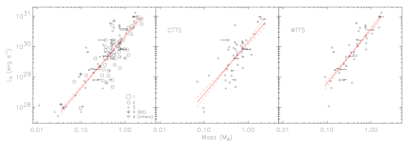
Figure 1: X-ray luminosity as a function of mass. From left to right: (a) For all stars. (b) For CTTS. (c) For WTTS. The straight lines indicate the regression curves (from the EM algorithm), and the dashed lines illustrate the errors in the slopes.

Source and background spectra have been obtained for each instrument using data during the Good Time Intervals (GTIs, i.e., intervals that do not include flaring background). Further, time intervals with obvious strong stellar flares were also excluded from the spectra in order to avoid bias of our results by episodically heated very hot plasma.

One PN spectrum usually provides more counts than the two MOS spectra together. We therefore only used the PN data for the spectral analysis, except for the sources for which PN data were not available (e.g., because the PN was not operational, or the sources fell into a PN CCD gap).

The spectral fits were performed using two different approaches in the full energy band. First, we have fitted the spectra using a conventional one- or two-component spectral model (1-$T$ and 2-$T$), both components being subject to a common photoelectric absorption. In this approach, the hydrogen column density, $N_{\rm H}$, two temperatures ($T_{1,2}$) and two emission measures (${\rm EM}_{1,2}$) are fitted in XSPEC (Arnaud, 1996) using the vapec thermal collisional-ionization equilibrium model.

In the second approach, the spectra were fitted with a model consisting of a continuous emission measure distribution (EMD) as found for pre-main sequence and active ZAMS stars (Telleschi et al., 2005; Argiroffi et al., 2004; García-Alvarez et al., 2005; Scelsi et al., 2005). The model consists of a grid of 20 thermal components binned to intervals of $d\log T=0.1$ from $\log T=6$ to $\log T=7.9$, arranged such that they form an EMD with a peak at a temperature $T_{\rm 0}$ and two power-laws toward lower and higher temperatures with power-law indices $\alpha$ and $\beta$, respectively. Given the poor sensitivity of CCD spectra at low temperatures, $\alpha$ was kept fixed at 2, consistent with values found in previous studies (Telleschi et al., 2005; Argiroffi et al., 2004), while we let $\beta$ free to vary (between $-3\leq\beta\leq 1$). The absorbing hydrogen column density $N_{\rm H}$ was also fitted to the data. The abundances were fixed at values typical for pre-main sequence stars or very active zero-age main-sequence stars (Telleschi et al., 2005; Argiroffi et al., 2004; García-Alvarez et al., 2005; Scelsi et al., 2005). For further details, see Güdel et al. (2006a).

For each star and each model we computed the average temperature ($T_{\rm av}$) as the logarithmic average of all temperatures used in the fit, applying the emission measures as weights. The X-ray luminosity ($L_{\rm X}$) was computed in the energy range 0.3-10 keV from the best-fit model assuming a distance of 140 pc.

Of the 126 members detected in XEST, 22 were detected in two different exposures. In those cases, two separate spectral fits were made. For correlations of X-ray parameters with stellar properties, we used logarithmic averages of the results from the two fits. On the other hand, if we correlate X-ray properties with each other, we treat the two spectral fit results from the same source as different entries.

Results from the spectral fits are given in Table 5 (for the EMD fits) and Table 6 (for the 1-$T$ and 2-$T$ fits) of Güdel et al. (2006a). We use the results from the EMD interpretation to perform statistical correlations below.

4 Results

Motivated by results from previous X-ray studies and in particular guided by the COUP work (Preibisch et al., 2005), we now seek systematics in the X-ray emission by correlating X-ray parameters first with fundamental stellar parameters, and then also seeking correlations among the X-ray parameters themselves. We will consider the fundamental stellar properties of mass and bolometric luminosity, accretion rate, and age, but we will not discuss rotation properties here (see Briggs et al. 2006 for a detailed study). The basic X-ray properties used for our correlations are the X-ray luminosity $L_{\rm X}$ in the 0.3-10 keV band and the average electron temperature $T_{\rm av}$. One of the main goals of this section is to seek differences between CTTS and WTTS. We will compare our findings with those of COUP and some other previous work in Sect. 5.

4.1 Correlations between X-rays and stellar parameters

4.1.1 Correlation with mass

In Fig. 1 we plot the X-ray luminosity, $L_{\rm X}$ (in erg s^-1), as a function of the stellar mass ($M$, in units of the solar mass, $M_{\odot}$, from Table 10 in Güdel et al. 2006a). In the left panel we show the relation for all types of objects in our sample. Different symbols are used to mark different object types (see panel in figure). Upper limits for non-detections are marked with arrows. In the middle and right panels the same relation is shown separately for CTTS and WTTS, respectively. A clear correlation is found between the two parameters in all three plots, in the sense that $L_{\rm X}$ increases with mass. The correlation coefficients are 0.79 for the whole sample (99 entries), 0.74 for the CTTS (45 entries), and 0.84 for the WTTS (43 entries). We computed the significance of the correlation using correlation tests in ASURV (LaValley et al. 1992; specifically, the Cox hazard model, Kendall’s tau, and Spearman’s rho have been used) and found a probability of $<0.01$% that the the parameters are uncorrelated in each of the three cases. As for all subsequent statistical correlation studies, we summarize these parameters in Table 1.

Table 1: Summary of results found for the different correlations. In the third column, n is the number of stars used in the statistic. $P$ is the probability that the parameters are uncorrelated (computed with ASURV), $C$ is the correlation coefficient and $\sigma$ is the standard deviation from the EM algorithm. The intercept of the linear regression is $a$, and $b$ is the slope. Errors are 1-sigma rms values for the respective variables.

Correlation	stellar	n	EM algorithm		bisector algorithm		P	C	$\sigma$
	sample
			$a$	$b$	$a$	$b$
$L_{\rm X}$ vs $M$	all	99	$30.33\pm 0.06$	$1.69\pm 0.11$	$30.44\pm 0.05$	$1.91\pm 0.11$	$<0.01$%	0.79	0.45
$L_{\rm X}$ vs $M$	CTTS	45	$30.13\pm 0.09$	$1.70\pm 0.20$	$30.24\pm 0.06$	$1.98\pm 0.20$	$<0.01$%	0.74	0.45
$L_{\rm X}$ vs $M$	WTTS	43	$30.57\pm 0.09$	$1.78\pm 0.17$	$30.69\pm 0.07$	$2.08\pm 0.17$	$<0.01$%	0.84	0.38
$T_{\rm av}$ vs $L_{\rm X}$	CTTS	19	$6.45\pm 2.31$	$0.01\pm 0.08$	$-17.95\pm 13.25$	$0.85\pm 0.45$	43-80%	0.06	0.22
$T_{\rm av}$ vs $L_{\rm X}$	WTTS	29	$2.53\pm 0.81$	$0.15\pm 0.03$	$0.13\pm 0.93$	$0.23\pm 0.03$	$<0.01$%	0.69	0.12
$T_{\rm av}$ vs $F_{\rm X}$	CTTS	18	$6.77\pm 0.76$	$0.05\pm 0.12$	$1.67\pm 1.11$	$0.86\pm 0.18$	62-42%	0.11	0.22
$T_{\rm av}$ vs $F_{\rm X}$	WTTS	32	$5.75\pm 0.20$	$0.18\pm 0.03$	$5.21\pm 0.24$	$0.26\pm 0.03$	$<0.01$%	0.72	0.11
$L_{\rm X}$ vs $L_{*}/L_{\odot}$	all	108	$30.00\pm 0.05$	$1.05\pm 0.06$	$30.07\pm 0.04$	$1.11\pm 0.05$	$<0.01$%	0.83	0.44
$L_{\rm X}$ vs $L_{*}/L_{\odot}$	CTTS	48	$29.83\pm 0.06$	$1.16\pm 0.09$	$29.89\pm 0.05$	$1.20\pm 0.10$	$<0.01$%	0.84	0.39
$L_{\rm X}$ vs $L_{*}/L_{\odot}$	WTTS	44	$30.22\pm 0.08$	$1.06\pm 0.10$	$30.31\pm 0.06$	$1.25\pm 0.09$	$<0.01$%	0.85	0.41
$L_{\rm X}/L_{\rm X}(\dot{M})$ vs $\dot{M}$	CTTS	37	$-4.05\pm 1.19$	$-0.48\pm 0.15$	$-8.32\pm 1.11$	$-1.02\pm 0.14$	$0.14-0.52$%	-0.47	0.57
$L_{\rm X}(M=1M_{\odot})$ vs age	all	93	$30.45\pm 0.06$	$-0.36\pm 0.11$	$30.69\pm 0.06$	$-1.02\pm 0.07$	$0.10-0.38$%	-0.31	0.44
$L_{*}/L_{\odot}$ vs $M$	all	113	$0.23\pm 0.04$	$1.49\pm 0.07$	$0.93\pm 0.04$	$1.65\pm 0.06$	$<0.01$%	0.90	0.31

We computed linear regression functions for the logarithms of the two parameters, of the form $\log y=a+b\log x$, using the parametric estimation maximization (EM) algorithm in ASURV, which implements the methods presented by Isobe et al. (1986). We find the regression functions $\log L_{\rm X}=(1.69\pm 0.11)\log M+(30.33\pm 0.06)$ for the full stellar sample, $\log L_{\rm X}=(1.70\pm 0.20)\log M+(30.13\pm 0.09)$ for the CTTS, and $\log L_{\rm X}=(1.78\pm 0.17)\log M+(30.57\pm 0.09)$ for the WTTS. The regression parameters are also listed in Table 1, as for all subsequent regression analyses. In the ONC sample, Preibisch et al. (2005) found the similar linear regression $\log L_{\rm X}=(1.44\pm 0.10)\log M+(30.37\pm 0.06)$ for all stars with masses $<2M_{\odot}$ using the same algorithm.

The EM algorithm is an ordinary least-square (OLS) regression of the dependent variable $y$ ($L_{\rm X}$ in this case) against the independent variable $x$ ($M$). When using this method, we assume that $L_{\rm X}$ is functionally dependent on the given mass (Isobe et al., 1990). However, the $M$ values are also uncertain, and assuming a functional dependence a priori may not be correct. We therefore also computed the linear regression using the bisector OLS method after Isobe et al. (1990), which treats the variables symmetrically. In this case, we find $\log L_{\rm X}=(1.91\pm 0.11)\log M+(30.44\pm 0.05)$ for all stars together, $\log L_{\rm X}=(1.98\pm 0.20)\log M+(30.24\pm 0.06)$ for the CTTS, and $\log L_{\rm X}=(2.08\pm 0.17)\log M+(30.69\pm 0.07)$ for the WTTS (see Table 1). The slopes for the bisector OLS are slightly steeper than in the EM algorithm. However, the values for CTTS and WTTS agree within one sigma, and we caution that the upper limits for non-detections are not taken into account in the bisector linear regression method.

We verified this trend for the subsample of stars that have not been recognized as multiples. We find the regression lines $\log L_{\rm X}=(1.72\pm 0.12)\log M+(30.39\pm 0.07)$ using the EM algorithm, and $\log L_{\rm X}=(1.85\pm 0.11)\log M+(30.48\pm 0.07)$ using the bisector algorithm. These results are fully consistent with the results for the total sample.

Differences are present between the CTTS and WTTS stellar samples. While the slopes found in the correlations for CTTS and WTTS are consistent within 1$\sigma$, the intercept of WTTS at 1$M_{\odot}(\log M/M_{\odot}=0)$ is $\approx 0.45$ dex larger than the intercept for CTTS. This lets us anticipate a larger average $L_{\rm X}$ in WTTS. The correlation is better determined for WTTS, as judged from a slightly higher correlation coefficient and a smaller error in the slope. Furthermore, the standard deviation, $\sigma$, of the points with respect to the regression function from the EM algorithm is slightly larger for CTTS (0.45) than for WTTS (0.38).

4.1.2 Evolution of X-ray emission

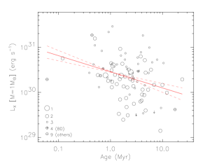
Figure 2: Evolution of the normalized X-ray emission. $L_{\rm X}$ has been normalized with the predicted values from the $L_{\rm X}$-mass relation (see text for details). The linear regression computed with the EM algorithm is plotted (solid line) together with errors in the slopes (dashed line). Symbols mark different types of stars.

Here, we discuss the evolution of the X-ray emission with age. Among main-sequence (MS) stars, $L_{\rm X}$ is correlated with rotation and anti-correlated with age. The common explanation is that magnetic activity is directly related to the stellar rotation, and the latter decays with age because of magnetic braking. However, TMC PMS stars do not show the relation between $L_{\rm X}$ and rotation observed for MS stars (Briggs et al., 2006). On the other hand, $L_{\rm X}$ decreases during the evolution of pre-main sequence stars, provided that a common X-ray saturation law applies (see below), because $L_{*}$ decreases along the Hayashi track.

We have found (see Sect. 4.1.1) that $L_{\rm X}$ shows a strong correlation with mass. In order to avoid an interrelationship between the correlations, we normalize the measured $L_{\rm X}$ with $L_{\rm X}(M)$ predicted by the correlation with mass ($L_{\rm X}(M)=10^{30.33}M^{1.69}$ erg s^-1) and multiply with the $L_{\rm X}$ expected for a 1 $M_{\odot}$ star ($10^{30.33}$ erg s^-1). We designate this quantity by $L_{\rm X}(M=1M_{\odot})$. In Fig. 2 we plot $L_{\rm X}(M=1M_{\odot})$ as a function of age. A slight decline in $L_{X}$ is found between 0.1 and 10 Myr. The correlation coefficient is $C=-0.31$ for 93 entries. The tests in ASURV give probabilities between 0.1% and 0.38% that age and $L_{\rm X}(M=1M_{\odot})$ are uncorrelated. We have computed a linear regression with the EM algorithm in ASURV and find $\log(L_{\rm X}/L_{\rm X}(M))=(-0.36\pm 0.11)\log\leavevmode\nobreak\ ({\rm age})+(30.45\pm 0.06)$ (where age is in Myr). Further, we have tested the linear regression and the correlation probability when we neglect the two youngest stars (V410 X4 and LkH$\alpha$ 358) and found the linear regression to be consistent within error bars with the above relation, with a probability of $P<1$% for no correlation. Further, as a test, we have computed the linear regression using the bisector algorithm. We find a much steeper slope of $-1.02\pm 0.07$ (Table 1), indicating that the linear regression is nevertheless only marginal, and the scatter is dominated by other contributions.

Preibisch & Feigelson (2005) reported correlations consistent with ours, applying the EM algorithm to the ONC data. They correlated $L_{\rm X}$ with age in mass-stratified subsamples of the surveyed stars and found $L_{\rm X}$ to decrease with age with slopes ranging from -0.2 to -0.5, i.e. fully consistent with the slope found in Fig. 2 (mass-stratified analysis for our sample also indicates decreasing $L_{\rm X}$ in some mass bins but not in others; our statistics are too poor for this purpose).

4.1.3 Mass accretion rates

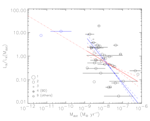
Figure 3: Residual X-ray luminosity for CTTS (after normalization with the $M-L_{\rm X}$ and $M-\dot{M}$ relation) as a function of the mass accretion rate. Regression lines obtained using the EM algorithm (red) and the bisector algorithm (blue) are plotted with their respective errors in the slope (dashed lines). The regression lines are computed only using the stars plotted with black circles, while the two stars with $\dot{M}$ smaller than $10^{-10}M_{\odot}$ yr^-1 were ignored (see text for more details).

Figure 4: Upper panel: Fractional X-ray luminosity vs. $\dot{M}$. Lower panel: $T_{\rm av}$ vs. $\dot{M}$. Different symbol sizes represent different object types as defined in the figures. Arrows represent upper limits for the accretion rates.

We now directly compare the X-ray parameters derived from our spectral fits ($L_{\rm X}$, $L_{\rm X}/L_{*}$, and $T_{\rm av}$) with the previously determined mass accretion rates ($\dot{M}$, in $M_{\odot}$ yr^-1). We use $\dot{M}$ listed in the XEST catalog (Güdel et al., 2006a, and references therein). Accretion rates may be variable, and various methods for their determination may produce somewhat different results. If different values were found for a given star in the literature, the range of $\dot{M}$ is marked by a horizontal line in our figures.

When comparing $L_{\rm X}$ with $\dot{M}$, some caution is in order. In Sect. 4.1.1 we have shown that a tight relation exists between $L_{\rm X}$ and the stellar mass. Further, a clear relation between $\dot{M}$ and the stellar mass has been found for class II objects in the literature (e.g., Muzerolle et al., 2003, 2005; Calvet et al., 2004). Combining the $L_{\rm X}$-mass and $\dot{M}$-mass relations, we expect $L_{\rm X}$ to correlate with $\dot{M}$ as well. However, here we are interested in testing if an intrinsic relation between the latter two parameters exists that is not a consequence of the two former relations. Calvet et al. (2004) have used evolutionary tracks of Siess et al. (2000) (consistent with the XEST survey) to find a relation $\dot{M}\propto M^{1.95}$ in the mass range between 0.02 and 3 $M_{\odot}$. Similarly, Muzerolle et al. (2003) and Muzerolle et al. (2005) found $\dot{M}\propto M^{2}$ and $\dot{M}\propto M^{2.1}$ respectively, using different evolutionary tracks. We therefore adopt the relation $\log\dot{M}\approx 2\log M-7.5$. Further, we use $\log L_{\rm X}=1.69\log M+30.33$ (Sect. 4.1.1), and we then compute the expected $L_{\rm X}$ for each $\dot{M}$ value, namely $\log L_{\rm X}(\dot{M})=0.85\log\dot{M}+36.67$.

In Fig. 3 we plot the ratio of $L_{\rm X}/L_{\rm X}(\dot{M})$ as a function of $\dot{M}$ for class II objects. We will expect that the values scatter around a constant if this ratio were determined only by the $M-L_{\rm X}$ and $M-\dot{M}$ relations. We find a very large scatter for any given $\dot{M}$ (2–3 orders of magnitude) but, using a regression analysis, a tendency for weak accretors to show higher $L_{\rm X}$, compared to strong accretors. However, if we exclude the two stars with the smallest accretion rates (plotted with blue symbols in Fig. 3), the correlation is less clear. In this case, the correlation coefficient is $C=-0.47$ for 37 data points. Nevertheless, the probability, computed in ASURV for the EM algorithm, that no correlation is present is only $P=$ 0.1% – 0.5%. We have computed the linear regression using different methods. With the EM algorithm we find $\log L_{\rm X}/L_{\rm X}(\dot{M})=(-0.48\pm 0.15)\log\dot{M}-(4.05\pm 1.19)$ (Table 1). Using the bisector algorithm, however, the slope is found to be $-1.02\pm 0.14$, i.e., more than 3 sigma steeper than the slope found with the EM algorithm. The entries for two stars with low $\dot{M}$ (plotted in blue) are consistent with the linear regression found with the EM algorithm. We conclude that the two parameters are not evenly distributed, but that a linear regression of the logarithmic values cannot clearly be claimed.

In Fig. 4 we plot $L_{\rm X}/L_{*}$ and $T_{\rm av}$ as a function of the accretion rate. Arrows represent upper limits for $\dot{M}$. In both cases no correlation is evident.

4.1.4 Correlation with bolometric luminosity

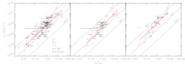
Figure 5: $L_{\rm X}$ as a function of the $L_{*}$. Left: for all stars; the different symbols describe different classes of stars, while arrows are upper limits for non-detections. Middle: same for CTTS (type 2). Right: same for WTTS (type 3). The horizontal bars show the ranges of literature values for $L_{*}$.

In Fig. 5 we plot $L_{\rm X}$ as a function of the stellar bolometric luminosity $L_{*}$ (from Güdel et al. 2006a and references therein). The lines corresponding to $L_{\rm X}/L_{*}=10^{-3},10^{-4}$, and $10^{-5}$ are also shown. In the left panel, all stars are plotted, with different symbols for each stellar class as described in the figure. We again excluded from the plot the stars mentioned in Sect. 2. Upper limits for non-detections are marked with arrows. By far most of the stars are located between $L_{\rm X}/L_{*}=10^{-3}$ and $L_{\rm X}/L_{*}=10^{-4}$. In the middle and right panels, we present CTTS and WTTS separately.

The correlation coefficients are 0.83 for the full stellar sample (108 entries), and 0.84 (48 entries) and 0.85 (44 entries) for CTTS and WTTS, respectively. Probabilities for the absence of a correlation are very small, $P<0.01$%. We computed linear regression lines with the EM algorithm in ASURV. For the full sample, we find $\log L_{\rm X}=(1.05\pm 0.06)\log L_{*}/L_{\odot}+(30.00\pm 0.05)$, whereas for CTTS and WTTS, $\log L_{\rm X}=(1.16\pm 0.09)\log L_{*}/L_{\odot}+(29.83\pm 0.06)$ and $\log L_{\rm X}=(1.06\pm 0.10)\log L_{*}/L_{\odot}+(30.22\pm 0.08)$, respectively. Fig. 5c shows one WTTS at $L_{*}/L_{\odot}\approx 0.01$ with a rather high $L_{\rm X}\approx 5\times 10^{29}$ erg s^-1 (KPNO-Tau 8 = XEST-09-022). Not considering this object, the slope of the regression slightly steepens to $1.17\pm 0.09$, which is only marginally different from the slope based on all WTTS. The standard deviation at the same time marginally decreases from 0.41 to 0.36.

Again, we also computed a linear regression using the bisector OLS algorithm that treats both $L_{*}$ and $L_{\rm X}$ as independent variables. The slopes are very similar to the those reported above (Table 1). The important distinction between CTTS and WTTS is that the latter clearly tend to be located at higher $L_{\rm X}/L_{*}$ (see also below): at $L_{*}/L_{\odot}=1$ the CTTS show an average $\log L_{\rm X}=29.83$  [erg s^-1], while for the WTTS, $\log L_{\rm X}=30.22$ [erg s^-1].

The regressions are thus compatible with a linear relation between $L_{\rm X}$ and $L_{*}$, and therefore $L_{\rm X}/L_{*}$ is, on average for a given $L_{*}$, a constant between $10^{-4}$ and $10^{-3}$ regardless of $L_{*}$. This is reminiscent of the situation among very active, rapidly rotating main-sequence or evolved subgiant stars that saturate at fractional X-ray luminosities of the same order, provided they rotate sufficiently rapidly. We thus find that the majority of our TTS are in a saturated state. A consequence of this would be that rotation no longer controls the X-ray output, as suggested by Preibisch et al. (2005) for the Orion sample. This is discussed for the XEST sample by Briggs et al. (2006). Below, we will specifically study whether the $L_{\rm X}/L_{*}$ relation is different for CTTS and for WTTS.

The correlation found for the full stellar sample is compatible with the relation found in Orion: $\log L_{\rm X}=(1.04\pm 0.06)\log(L_{*}/L_{\odot})+(30.00\pm 0.04)$ (Preibisch et al., 2005). The slope found for the WTTS in the ONC is also consistent with our results within the error bars. For CTTS, on the other hand, Preibisch et al. (2005) found a very large scatter in the correlation. This is not observed in our XEST sample; we rather see similar scatter for CTTS and WTTS, as demonstrated by the similar correlation coefficients, the similar errors in the slope, and the similar standard deviations. Preibisch et al. (2005) suggested that strong accretion could lead to larger errors in the determination of stellar luminosity and the effective temperature.

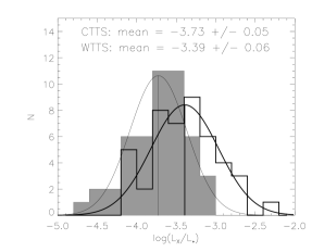
Figure 6: Distributions of $\log(L_{\rm X}/L_{*})$ for CTTS (grey histogram) and WTTS (white histogram). Gaussians that fit the distributions are also plotted and their peaks are marked with vertical lines.

Figure 7: Cumulative distribution of $\log(L_{\rm X}/L_{*})$ for CTTS (solid) and for WTTS (dotted).

Figure 8: Cumulative distributions of $\log(L_{\rm X}/L_{*})$ for WTTS (dotted) and CTTS (solid) for masses smaller than 0.3 $M_{\odot}$ (left), masses between 0.3 and 0.7 $M_{\odot}$ (middle), and masses larger than 0.7 $M_{\odot}$ (right).

4.1.5 Fractional X-ray luminosity $L_{\rm X}/L_{*}$

In Fig. 6 we plot the histogram for the distribution of $\log(L_{\rm X}/L_{*})$ for CTTS (grey) and WTTS (white). The two populations are different, with WTTS having a larger mean $\log(L_{\rm X}/L_{*})$. We fitted each of the two histograms with a Gaussian function and computed the mean and its errors. For CTTS, we find $\langle\log(L_{\rm X}/L_{*})\rangle=-3.73\pm 0.05$, while for WTTS, $\langle\log(L_{\rm X}/L_{*})\rangle=-3.39\pm 0.06$.

A more rigorous test is based on the Kaplan-Meier estimators as computed in ASURV, which implements the methods presented by Feigelson & Nelson (1985). This method also accounts for the upper limits in $L_{\rm X}$ for the non-detections. The results are plotted in Fig. 7. The solid line represents the CTTS, the dotted line the WTTS. The WTTS distribution is shifted toward larger $\log(L_{\rm X}/L_{*})$ compared to the CTTS distribution by a factor of approximately 2. We find $\langle\log(L_{\rm X}/L_{*})\rangle=-3.72\pm 0.06$ and $\langle\log(L_{\rm X}/L_{*})\rangle=-3.36\pm 0.07$ for CTTS and WTTS, respectively, in full agreement with the Gaussian fit. Judged from a two-sample test based on the Wilcoxon test and logrank test in ASURV, the probability that the two distributions are obtained from the same parent population is very low, namely $P=0.01$%$-0.03$%.

Again, we test this result using the subsample of stars that have not been recognized as multiples. The subsample consists on 29 CTTS (4 of which have upper limits) and 33 WTTS (with no upper limits). We find a probability of $P=0.05$%$-0.07$% that the distributions arise from the same parent population, and $\langle\log(L_{\rm X}/L_{*})\rangle_{\rm CTTS}=-3.83\pm 0.06$ and $\langle\log(L_{\rm X}/L_{*})\rangle_{\rm WTTS}=-3.40\pm 0.08$. These results are consistent with the results found in the full sample. We can therefore conclude that multiplicity does not influence our results.

In Fig. 8 we plot the Kaplan-Meier estimator for the distribution of $\log(L_{\rm X}/L_{*})$ in three different mass ranges: for stars with masses smaller than 0.3 $M_{\odot}$, between 0.3 and 0.7 $M_{\odot}$, and larger than 0.7 $M_{\odot}$. For the latter two mass bins, the distributions belong to two different parent populations at the $>94$% level. For lower masses ($M<0.3M_{\odot}$), we find the CTTS and WTTS distributions to be similar, but we still find larger $\log(L_{\rm X}/L_{*})$ for WTTS than than for CTTS. The difference between the two populations is not significant at the $\approx$ 10% level possibly because of the small size of the stellar sample in this mass range.

Our results can be compared with the distributions found in the COUP survey, shown in Fig. 16 of Preibisch et al. (2005). In the latter figure, the stars are classified according to the 8542 Å Ca II line, which is an indicator of disk accretion, similar to the EW(H$\alpha$) used in our work. In Orion, a substantial difference has been found between the distributions of accreting and non-accreting stars in the mass ranges 0.2–0.3 $M_{\odot}$ and 0.3–0.5 $M_{\odot}$. However, for 0.5–1 $M_{\odot}$, the two distributions appeared to be compatible, in contrast to our findings that show fainter CTTS consistently in all mass ranges.

Figure 9: X-ray Luminosity Function (XLF) for CTTS (solid) and WTTS (dotted) for for masses smaller than 0.3 $M_{\odot}$ (left), masses between 0.3 and 0.7 $M_{\odot}$ (middle), and masses larger than 0.7 $M_{\odot}$ (right).

Figure 10: X-ray Luminosity Function (XLF) for CTTS (solid) and WTTS (dotted).

4.2 Correlations between X-ray parameters

4.2.1 The X-ray luminosity function

In Fig. 10 we display the X-ray luminosity function (XLF) for WTTS and CTTS for our Taurus sample. The XLF has again been calculated using the Kaplan-Meier estimator in ASURV, so that the few upper limits have also been considered. The total number of sources used was 105, 56 of them being CTTS (including 6 upper limits) and 49 WTTS (including 1 upper limit). The WTTS are again more luminous than CTTS by a factor of about 2 (with mean values $\langle\log L_{\rm X}\rangle_{\rm C}=29.51$ and $\langle\log L_{\rm X}\rangle_{\rm W}=29.80$). The probability that the two distributions arise from the same parent population is $7$%$-10$%, computed using ASURV as described in Sect. 4.1.5.

If we restrict the stellar sample to stars with no recognized multiplicity, we obtain average X-ray luminosities of $\langle\log L_{\rm X}\rangle_{\rm C}=29.38$ and $\langle\log L_{\rm X}\rangle_{\rm W}=29.65$, for samples consisting of 32 CTTS (5 upper limits) and 36 WTTS (1 upper limit). The difference between the two stellar samples is 0.3 dex (i.e., a factor of two), similar to what we found for the full sample. However, the two-sample tests give a larger probability (P = 12%–33%) that the two stellar groups arise from the same parent population. Among the multiple sources, 24 are CTTS (with 1 upper limit), but only 13 are WTTS (with no upper limit). By adding the multiples to the sample of single stars, we expect that the distributions slightly shift toward larger $L_{\rm X}$, and because there are significantly more multiple CTTS, the CTTS distribution of the total sample should be more similar to the WTTS total distribution, but the opposite trend is seen. We conclude that the trends are grossly the same for the total sample and the single-star subsamples, the larger probability being due to significantly smaller samples that are compared. Overall, thus, CTTS are recognized as being X-ray deficient when compared to WTTS.

Fig. 9 shows the X-ray luminosity function for the same three mass ranges as used in Sect. 4.1.5 ($M<0.3M_{\odot}$ in the left panel, $0.3M_{\odot}<M<0.7M_{\odot}$ in the middle panel, and $M>0.7_{\odot}$ in the right panel). Again, we find the largest difference between CTTS and WTTS for the two higher-mass bins, with probabilities of only $2$%$-4$% that the distributions belong to the same parent population. The probability is substantially larger for $M<0.3M_{\odot}$ ($29$%$-32$%), but the statistics are also considerably poorer.

Considering the difference in the XLFs of CTTS and WTTS alone, a possible cause could be that the bolometric luminosity function of CTTS would indicate lower luminosities $L_{*}$ than for WTTS, which would result in lower average $L_{\rm X}$ provided that $L_{\rm X}/L_{*}\approx$ constant, i.e., that saturation applies for all stars. In Fig. 11, we plot the distributions of $L_{*}$ for WTTS and CTTS. In fact, the CTTS are found to be slightly more luminous than the WTTS. We find $\langle\log L_{*}\rangle_{C}=33.35\pm 0.08$ and $\langle\log L_{*}\rangle_{W}=33.19\pm 0.09$. The probability that the distributions arise from the same parent population is $15$%$-21$%, i.e. making the difference marginal. We conclude that because $L_{\rm X}$ is linearly correlated with $L_{*}$ (Fig. 5), the difference in $L_{\rm X}$ for the two samples is intrinsic, which is of course a reconfirmation of our previous finding that the distributions of $L_{\rm X}/L_{*}$ also indicate lower activity for CTTS compared to WTTS.

Figure 11: Stellar bolometric luminosity function for CTTS (solid) and WTTS (dotted).

4.2.2 Absorption

In Fig. 12 we plot the distribution of $N_{\rm H}$ for accreting (solid line) and non-accreting stars (dotted line) calculated using the Kaplan-Meier estimator in ASURV. The logarithmic average of $N_{\rm H}$ for CTTS is $\langle N_{\rm H}\rangle_{C}=4.2\times 10^{21}$ cm^-2 and is more than a factor of two larger than the average for WTTS ($\langle N_{\rm H}\rangle_{W}=1.8\times 10^{21}$ cm^-2).

The $N_{\rm H}$ values found from our spectral fits are roughly consistent with the visual extinctions $A_{\rm V}$ and the infrared extinctions $A_{\rm J}$ if we assume a standard gas-to dust ratio ($N_{\rm H}/A_{\rm V}=2\times 10^{21}\leavevmode\nobreak\ {\rm cm}^{-2}\leavevmode\nobreak\ {\rm mag}^{-1}$, $N_{\rm H}/A_{\rm J}=7.1\times 10^{21}\leavevmode\nobreak\ {\rm cm}^{-2}\leavevmode\nobreak\ {\rm mag}^{-1}$; Vuong et al. 2003). For a detailed discussion on the gas-to-dust ratio in TMC, we refer the reader to Glauser et al. (2007, in preparation). High photoelectric absorption might influence the spectral fits to low-resolution spectra, because the coolest plasma components, more affected by absorption, cannot be reliably quantified.

Figure 12: Cumulative distribution of $N_{\rm H}$ for CTTS (solid line) and WTTS (dotted line).

We studied possible biases introduced by high absorption by correlating $N_{\rm H}$ with $T_{\rm av}$ and $L_{\rm X}$. We have found $L_{\rm X}$ to range between approximately $10^{28}$ erg s^-1 and $10^{31}$ erg s^-1, independent of the photoelectric absorption. The uncertainty of the determination of $L_{\rm X}$, on the other hand, does increase with increasing $N_{\rm H}$ (and decreasing number of counts in the spectrum) as derived by Güdel et al. (2006a). Similarly, if we correlate $T_{\rm av}$ with $N_{\rm H}$ (Fig. 13), we find a larger range of $T_{\rm av}$ (symmetrically around $\log T_{\rm av}\approx 7.0$ [K]) for highly absorbed sources, while $T_{\rm av}$ is found to be similar for all the sources with low absorption ($N_{\rm H}<10^{21}$ cm^-2), $\log T_{\rm av}\approx 7.0\pm 0.2$ [K]. The larger range of $T_{\rm av}$ at higher $N_{\rm H}$ is likely to be the result of larger scatter due to less reliable spectral fitting. In any case, there is no trend toward higher $T_{\rm av}$ for higher $N_{\rm H}$.

Figure 13: $T_{\rm av}$ as a function of $N_{\rm H}$ for our sample.

4.2.3 Correlation of $L_{\rm X}$ with electron temperature

In Fig. 14 we plot $T_{\rm av}$ as a function of $L_{\rm X}$ and as a function of the X-ray surface flux ($F_{\rm X}$) for CTTS and WTTS, respectively. The surface fluxes have been calculated using the radii reported in Table 10 of Güdel et al. (2006a). In the plots for the WTTS we also show values for six main-sequence G-type solar analog stars (Telleschi et al., 2005), for 5 K-type stars (AB Dor from Sanz-Forcada et al. 2003, and $\epsilon$ Eri, 70 Oph A&B, 36 Oph A&B from Wood & Linsky 2006), and for 6 M-type main-sequence stars (EQ Peg, AT Mic, AD Leo and EV Lac from Robrade & Schmitt 2005, AU Mic from Magee et al. 2003, and Proxima Cen from Güdel et al. 2004).

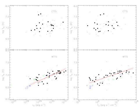
Figure 14: Left pannel: $T_{\rm av}$ as a function of $L_{\rm X}$ for CTTS (top) and WTTS (bottom). Right panel: $T_{\rm av}$ as a function of $F_{\rm X}$ for CTTS (top) and WTTS (bottom). The low-absorption TTS samples are marked by filled black bullets, while small crosses give loci of high-absorption objects or sources with few counts (see text for details). Black diamonds mark solar analog stars (Telleschi et al., 2005) and blue and green diamonds mark K- and M-type main-sequence stars, respectively (see text for references). The straight lines in the WTTS plots are linear regression fits (based on bisector regression, the dashed lines illustrating the error ranges in the slopes).

Spectral fits to low-resolution spectra that are subject to photoelectric absorption tend to ignore the coolest plasma components, as the soft part of the spectrum is most severely affected by the absorption. CTTS are on average more absorbed than WTTS. Given the larger absorptions, there could be a bias toward higher average temperatures in CTTS, although such a trend is not visible in Fig. 13. We nevertheless counteract a possible residual bias by restricting the stellar sample used for the correlation to stars with $N_{\rm H}<3\times 10^{21}$ cm^-2. The logarithmic means of $N_{\rm H}$ for CTTS and WTTS after these restrictions are $1.2\times 10^{21}$ cm^-2 and $8\times 10^{20}$ cm^-2, respectively, making these samples very similar with regard to absorption properties.

Further, we exclude the very faint sources (with less than 100 counts collectively in the three detectors) that could also produce unreliable $L_{\rm X}$ and $T_{\rm av}$ results. In Fig. 14 the filled circles represent the stars used for the linear regression fit, while the stars excluded from the fit are plotted with small crosses. Overall, the absorbed and faint sources fit well to the trends found from less absorbed and more luminous sources, but their scatter tends to be larger.

For CTTS, we find almost no correlation between $T_{\rm av}$ and $L_{\rm X}$ or $F_{\rm X}$ (the correlation coefficients are 0.06 and 0.11, respectively). On the contrary, for WTTS $T_{\rm av}$ is clearly correlated with both $L_{\rm X}$ and $F_{\rm X}$. The correlation coefficients are 0.69 and 0.72 for $L_{\rm X}$ and $F_{\rm X}$, with 33 and 32 data points, respectively (Table 1). The probability that no correlation is present is $<1$% in either case. We computed the linear regression using the bisector OLS algorithm (no a priori relation between the two measured variables assumed) to find $\log T_{\rm av}=(0.23\pm 0.03)\log L_{\rm X}+(0.13\pm 0.93)$ and $\log T_{\rm av}=(0.26\pm 0.03)\log F_{\rm X}+(5.21\pm 0.24)$. WTTS follow a trend similar to that shown by MS stars in the $T_{\rm av}$ vs. $L_{\rm X}$ relation. In the $T_{\rm av}$ vs. $F_{\rm X}$ relation, on the other hand, we find that WTTS are in general hotter than MS stars for a given $F_{\rm X}$.

We have checked these results using the EM algorithm, finding slightly shallower slopes (see Table 1). Shallower slopes are expected in the EM algorithm when compared to the bisector OLS algorithm (Isobe et al., 1990). For CTTS, where no correlation is found, the two algorithms result in completely different slopes (Table 1), an indication of absence of a linear regression (Isobe et al. 1990; the different slopes in the absence of a correlation are a consequence of the defining minimization of the algorithm. The EM algorithm returns a slope of $\approx 0$, whereas the bisector algorithm yields a slope around unity).

We use the Kaplan-Meier estimator in ASURV to compare the distributions of $T_{\rm av}$ for CTTS and WTTS. The two distributions are shown in Fig. 15 for the case where we do not apply a restriction to $N_{\rm H}$: the solid line represents CTTS, while the dotted line represents WTTS. Only stars with more than 100 counts in the three EPIC detectors are used. The probability that the two distributions arise from the same parent population is $0.7$%$-2$%. If we restrict the sample to stars with low $N_{\rm H}$ ($<3\times 10^{21}$ cm^-2), we find the mean value of $\log T_{\rm av}$[MK] $=7.10$ [MK] with $\sigma=0.22$ for CTTS and $\log T_{\rm av}$[MK] $=6.88$ with $\sigma=0.17$ for WTTS. The distribution is similar to the one found in Fig. 15 and the probability for the CTTS and WTTS distributions to originate from the same parent population is again only $0.7$%$-2$%.

We have checked if the difference found in the plasma temperatures of WTTS and CTTS could be attributed to abundance anomalies that may not have correctly been accounted for in the spectral fits. Kastner et al. (2002), Stelzer & Schmitt (2004), and Drake et al. (2005) found large Ne/Fe and Ne/O abundance ratios in the spectrum of TW Hya. We have therefore fitted the spectra of the 19 CTTS with $N_{H}<3\times 10^{21}$ cm^-2 and more than 100 counts in the combined EPIC spectra (filled black bullets in Fig. 14) adopting abundances as found in TW Hya (O = 0.2, Ne = 2.0, Fe = 0.2, with respect to the solar photospheric abundances of Anders & Grevesse 1989, all other abundances as given in Sect. 3). The average temperatures obtained with this model are generally consistent within 0.1 dex with the temperatures found based on our standard abundances. Only for one star, HO Tau AB, did we find an average temperature significantly lower, while the general trend toward higher $T_{\rm av}$ for CTTS remains unchanged. We can therefore exclude that the difference in temperatures is induced by abundance anomalies as those observed in TW Hya.

Telleschi et al. (2006a) derived the thermal structure of nine pre-main sequence stars from XEST based on high-resolution Reflection Grating Spectrometer data, using variable abundances. They found $T_{\rm av}$ to be compatible with values used here, which were derived from EPIC CCD spectra (an exception is the CTTS SU Aur, for which the temperature found with RGS is even higher than that derived from the EPIC spectra). In the latter work, however, a difference in the abundances has been found between stars of spectral type K and stars of spectral type G. The abundances found for the K-type stars reflect approximately the abundances used for the XEST EPIC fits (following an inverse FIP effect), while G-type stars show lower Ne/Fe and O/Fe abundance ratios. We therefore fitted the four G-type stars in our stellar sample with an abundance pattern as found for this spectral class by Telleschi et al. (2006a). Again, we did not find a significant change in temperatures. In summary, we do not find any appreciable effect that abundance anomalies other than those adopted in our study might have on the temperature determination. We also note that Scelsi et al. (2006, in preparation) studied the abundances derived from the EPIC spectra of the brightest sources in the XEST sample and found average abundances very similar to the standard abundances used in our CCD fits.

The difference in the coronal temperatures of CTTS and WTTS is in particular due to the larger $T_{\rm av}$ found in the CTTS with low $L_{\rm X}$. We therefore calculated the mean of all $T_{\rm av}$ values for CTTS and WTTS with $L_{\rm X}<3\times 10^{29}$ erg s^-1, low absorption ($N_{\rm H}<3\times 10^{21}$ cm^-2), and more than 100 counts in the three detectors. For these stars, we computed the errors in $T_{\rm av}$ as follows: We determined the 68% confidence contour on the $\beta-T_{0}$ plane for these two “parameters of interest”, i.e. the loci for which a fit can be achieved whose $\chi^{2}$ is larger by $\Delta\chi^{2}=2.3$ (1 $\sigma$) than the $\chi^{2}$ of the best fit. We then found the minimum and the maximum $T_{\rm av}$ for this subset of models, and thus defined the error range for $T_{\rm av}$. Using these errors, we computed the weighted mean of $\log T_{\rm av}$. For CTTS, we neglected DD Tau AB, which shows extraordinarily high temperatures in two different observations (two bullets at the hottest temperature in Fig. 14). For CTTS, we find $\langle\log T_{\rm av}\rangle=6.97\pm 0.06$ ($6.98\pm 0.06$ if DD Tau AB is also considered) while for WTTS we find $\langle\log T_{\rm av}\rangle=6.81\pm 0.05$. We therefore conclude that the CTTS and WTTS with $L_{\rm X}<3\times 10^{29}$ erg s^-1 are different at a 3$\sigma$ level, fully supporting the significant differences in the regression fits that are based on the entire $L_{\rm X}$ range.

In conclusion, we find the CTTS X-ray sources to be hotter than WTTS at a confidence level of $\gtrsim 98$%, and this result is partly due to the presence of a $L_{\rm X}-T_{\rm av}$ relation for WTTS but its absence in CTTS. Further, the WTTS relation coincides with relations valid for main-sequence stars of different spectral types, including saturated and non-saturated stars at different evolutionary stages.

Figure 15: Kaplan-Meier estimator for $T_{\rm av}$ for CTTS (solid) and WTTS (dotted). Only sources with more than 100 counts in the three EPIC detectors are used.

5 Discussion

5.1 Summary of trends

We now discuss the trends and correlations described in the previous section and will also put them into a context with previous reports, in particular from the COUP project.

The most significant correlations that we reported above are those between stellar mass and $L_{\rm X}$ (slope $\approx$ 1.7), between stellar bolometric luminosity $L_{*}$ and $L_{\rm X}$ (slope $\approx 1$), and between $L_{\rm X}$ and average electron temperature $T_{\rm av}$ (slope 0.15–0.23), the latter applying only to WTTS.

Further, we have found that $L_{\rm X}$ and $L_{\rm X}/L_{*}$ are both lower, on average, for CTTS than for WTTS, each by a factor of $\approx 2$, compatible with the finding that the distributions of $L_{*}$ are similar for the two samples. In contrast, $T_{\rm av}$ is, on average, higher by a factor of $\approx 1.7$ for CTTS than for WTTS.

Finally, we have studied possible correlations between $L_{\rm X},T_{\rm av}$, or $L_{\rm X}/L_{*}$ and the accretion rate but found at best unconvincing correlations. The same is true for a trend between $L_{\rm X}$ and age.

5.2 Comparison with previous studies

The $L_{\rm X}$ – mass correlation. This relation has been reported prior to XMM-Newton and Chandra studies of star-forming regions, but with largely varying regressions. Feigelson et al. (1993) found a slope of $3.6\pm 0.6$ for a sample of low-mass stars in the Chamaeleon I dark cloud based on ROSAT observations. There may be problems with more numerous upper limits at the low-mass (and low-luminosity) end of the distribution in this study, as noticed by Preibisch et al. (2005). On the other hand, the COUP sample reveals a very similar correlation to ours, with a slope only marginally smaller ($1.44\pm 0.10$) than for XEST ($1.69\pm 0.11$). The TMC sample thus essentially confirms the COUP results, and the residual difference might be due to a somewhat different distribution of stars in the HRD, perhaps indicating a different age distribution, as suggested from our discussion of this relation below.

A clear difference between the two studies is seen in the scatter around the regression curves. While Preibisch et al. (2005) report a standard deviation of 0.65 dex (factor of 4.5) around the best-fit line, we find for the XEST sample values between 0.38 (factor of 2.4, for WTTS) and 0.45 (factor of 2.8, for CTTS). We do not have a clear explanation for the smaller scatter in XEST, but note that i) similar findings apply to other correlations discussed below, and ii) the scatter found in the XEST results is close to the intrinsic uncertainties of any $L_{\rm X}$ measurement of magnetically active stars as these commonly vary by such factors on various time scales; Preibisch et al. (2005) give a factor of 2 variation on long (yearly) time scales for the Orion sample. We are thus confident that the quality of our mass – $L_{\rm X}$ correlation corresponds to the minimum scatter that must be expected from snapshot observations of magnetically active stars.

The $L_{\rm X}-L_{*}$ correlation. The linear correlation between these variables expresses the classical result of X-ray saturation that has been found empirically for main-sequence stars (Vilhu & Rucinski, 1983). A similar law applies to very active main-sequence and subgiant stars (see review by Güdel 2004 and references therein), and certainly also to pre-main sequence stars at various evolutionary stages (Flaccomio et al., 2003b). Again, the COUP study is in complete agreement with our results, its regression slope being $1.04\pm 0.06$. There is, however, a significant difference between the XEST and the COUP studies once CTTS and WTTS are treated separately. Preibisch et al. (2005) find a well-defined linear correlation for WTTS (standard deviation around best-fit regression of 0.52 dex), while for CTTS the scatter dominates (standard deviation = 0.72 dex) and the relation is significantly flatter. The CTTS data points span a range of 3 orders of magnitude at a given $L_{*}$. In XEST, the standard deviation of the scattered points is only $\approx 0.4$ dex for CTTS, WTTS, and the entire sample, with a range of $L_{\rm X}$ values at a given $L_{*}$ of about 1.5 dex. We are again not in a situation to explain the much tighter correlations for the XEST survey, but note that our spectral-fit methodology may suppress numerical uncertainty introduced by photoelectric absorption that suppresses evidence of plasma components at lower temperatures. Because we used an emission-measure distribution with a prescribed low-temperature shape as usually found in magnetically active stars, the presence of the coolest components is interpreted based on the presence of well-detected hotter plasma. An error analysis for $L_{\rm X}$ based in particular on $N_{\rm H}$ shows that for 76% of the sources in XEST, the intrinsic error range in $L_{\rm X}$ due to $N_{\rm H}$ is smaller than a factor of 3 (0.5 dex, in fact mostly much smaller), and the largest errors are obtained for faint sources subject to $N_{\rm H}>(2-3)\times 10^{21}$ cm^-3 (Güdel et al., 2006a). We note that Preibisch et al. (2005) used an X-ray luminosity averaged over the 10 days of exposure by Chandra, while in the XEST sample we have neglected time intervals containing obvious flares. However, Preibisch et al. (2005) found that the average $L_{\rm X}$ and the quiescent (“characteristic”) $L_{\rm X}$ differ by a median factor of 0.78, which would not be sufficient to explain the large scatter found in their $L_{\rm X}-L_{*}$ correlation for CTTS.

Comparison with main-sequence stars. Preibisch et al. (2005) also compare their $L_{\rm X}-L_{*}$ correlation with field main-sequence stars, and find a much shallower slope for the latter, but also a very large scatter. They similarly compare the $L_{\rm X}-$ mass relations with field stars, but there, they find a similar slope in the regression. We will not perform this comparison here, for the following reason. Field stars are found at various evolutionary stages, and as a consequence of stellar spin-down with age, the X-ray activity is subject to an evolutionary decay. Solar analogs decrease in $L_{\rm X}$ by three orders of magnitude from the zero-age main sequence to the end of the main-sequence life (Güdel et al., 1997; Telleschi et al., 2005). Further, the evolutionary speed is different for G stars and low-mass M dwarfs, the latter remaining at relatively high activity levels for a longer time (see Figs. 40 and 41 in Güdel 2004). Much of the scatter in $L_{\rm X}$ for a given mass or a given $L_{*}$ is thus due to mass-dependent evolutionary decay, and any trend in $L_{\rm X}$ vs. $L_{*}$ depends on the stellar age distribution. In contrast, both in active main-sequence stars and TTS, no evolutionary effects are expected for the $L_{\rm X}-L_{*}$ relation if the stars are in a saturated regime, and therefore $L_{\rm X}\propto L_{*}$.

For the $L_{\rm X}$ – mass relation, the scatter in $L_{\rm X}$ for a given mass is only about one order of magnitude; this scatter is indirectly due to the scatter in $L_{*}$ in the sample, due to different ages of stars of similar mass that contract vertically along the Hayashi track, provided that the X-ray emission remains in a saturated state (see HRD in Fig. 11 in Güdel et al. 2006a). The scatter in $L_{\rm X}$ due to evolution on the main sequence is much larger (3 orders of magnitude) and is due to intrinsic decay of the dynamo due to stellar spin down when the X-ray emission is no longer in a saturated state.

The $L_{\rm X}-T_{\rm av}$ correlation. A dependence between coronal electron temperature and emission measure or $L_{\rm X}$ (or normalized quantities such as the specific emission measure or surface X-ray flux) has first been noted by Vaiana (1983) and Schrijver et al. (1984). Quantitatively, for solar analogs, $L_{\rm X}\propto T^{4.5\pm 0.3}$ (Güdel et al. 1997, see Güdel 2004 for a review). For the pre-main sequence sample in the COUP survey, Preibisch et al. (2005) report a steep increase of the X-ray surface flux with the hotter temperature of their 2-component spectra, namely $F_{\rm X}\propto T_{2}^{6}$. On the other hand, they find a relatively constant lower temperature, namely $T_{1}\approx 10$ MK. In our study, we apply a more physically appropriate continuous emission measure distribution that does not distinguish between two isothermal components but that shows two power-law slopes on either side of the peak. The distribution of the logarithmically averaged temperatures (Fig. 15) does not show a preferred value but a smooth distribution in the range 4–30 MK around a mean of 7.6 MK for WTTS and 12.6 MK for CTTS (Sect. 4.2.3). Our regression curve for the $L_{\rm X}-T_{\rm av}$ indicates $L_{\rm X}\propto T_{\rm av}^{4.3-6.7}$ and $F_{\rm X}\propto T_{\rm av}^{3.8-5.6}$, compatible with the solar-analog relation as well as with the COUP relation for $T_{2}$. We note, however, that we find this trend only for WTTS (no separate analysis was provided for COUP).

$\log(L_{\rm X}/L_{*})$ distributions. Our distributions show the fractional X-ray luminosity of CTTS to be suppressed by a factor of $\approx 2$ compared to WTTS, with a mean $\log(L_{\rm X}/L_{*})\approx-3.39\pm 0.06$ and $-3.73\pm 0.05$ for WTTS and CTTS, respectively. These values agree excellently with those of COUP: $\log(L_{\rm X}/L_{*})\approx-3.31$ and $-3.73$ for WTTS and CTTS, respectively (Preibisch et al., 2005). XEST contrasts with COUP in that CTTS are less X-ray efficient for all considered mass bins, whereas Preibisch et al. (2005) found no difference in the ranges 0.1-0.2 $M_{\odot}$ and 0.5-1 $M_{\odot}$.

5.3 The $L_{\rm X}$ – mass relation

Among the clearest correlations we have identified is the $L_{\rm X}$-mass relation that closely corresponds to the finding in the COUP study. We now test the following: If we assume that TTS are in a saturated state (i.e. $L_{\rm X}\propto L_{*}$, Fig. 5) and a relation between $L_{*}$ and stellar mass exists (related to the age distribution of the stars and details of the evolution along the pre-main-sequence tracks), then the relation between $L_{\rm X}$ and mass could simply be a consequence of these two relations. Main-sequence stars follow the well-known mass-bolometric luminosity relation, which for stars in the mass range of 0.1–1.5$M_{\odot}$ reads $L_{*}\propto M^{3.0}$ (from a regression analysis using the Siess et al. 2000 ZAMS data). For pre-main sequence stars, a mass-bolometric luminosity relation is not obvious; during the contraction phase, a star of a given mass decreases its $L_{*}$ by up to 2 orders of magnitude. However, if most stars in a sample show similar ages, then an approximate mass-$L_{*}$ relation may apply to the respective isochrone. Fig. 16 illustrates the measured relation between $L_{*}$ and mass. The relation is rather tight, with a correlation coefficient of 0.90 for 113 sources. The Y/X OLS regression gives $\log L_{*}/L_{\odot}=(1.49\pm 0.07)\log M+(0.23\pm 0.04)$, with a standard deviation of 0.31. This relation can be compared with the theoretical prediction for an average isochrone appropriate for the XEST sample. We found that the logarithmically averaged age of our targets is 2.4 Myr. Adopting the Siess et al. (2000) isochrones, we find, from a linear regression fit, a dependence $L_{*}\propto M^{1.24}$, i.e., similar to the observed dependence and thus supporting our interpretation. We note that the XEST sample is of course not located on an isochrone (see Fig. 11 in Güdel et al. 2006a), and that other evolutionary calculations may lead to somewhat different slopes of the isochrones.

Adopting $\log(L_{\rm X}/L_{*})=-3.5$ for our entire TTS sample (see Fig. 5), we infer a relation $\log L_{\rm X}=1.49\log M+30.31$, similar to the correlation found in Sect. 4.1.1. In Fig. 17 we plot $L_{\rm X}$ as a function of mass after normalizing the observed $L_{\rm X}$ with $L_{\rm X}$ predicted from the above formula. The correlation found in Fig. 1 now disappears completely. The scatter in Fig. 17 is due to the scatter in Fig. 5 and in Fig. 16, i.e., intrinsic scatter not due to $L_{*}$ or $M$, but for example due to the evolutionary decrease of $L_{*}$ and $L_{\rm X}$ along the Hayashi track for a given mass.

We therefore conclude that the $L_{\rm X}$-mass relation is not an intrinsic relation but a consequence of an approximate mass-luminosity relation for stars with similar ages, combined with a saturation law.

Comparing the stars in the HRD of the TMC (Fig. 11 in Güdel et al. 2006a) with the HRD of the ONC sample (Fig. 1 in Preibisch et al. 2005), we note that the ONC sample is somewhat younger, although it is not tightly arranged along one isochrone, but tends to show a somewhat flatter slope than the TMC sample. The slightly shallower $L_{\rm X}$-mass relation in Preibisch et al. (2005) may therefore be a straightforward consequence of the younger average age of the ONC sample.

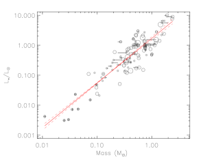
Figure 16: Stellar bolometric luminosity as a function of mass. The straight line is a Y/X OLS regression fit; dashed lines illustrate the 1-sigma errors in the slope.

Figure 17: $L_{\rm X}$ as a function of mass after renormalizing $L_{\rm X}$ with the expected $L_{\rm X}$ based on mass-bolometric luminosity relation and the saturation law (see text for details). Different symbols mark different types of stars.

5.4 Origin of the X-ray emission: CTTS vs WTTS

The question that we address in this section is on the origin of the X-ray emission. How do CTTS and WTTS differ, and what may be the causes? Where and how are the X-rays formed?

The relevant relations we have identified in this paper are the following: i) CTTS show, on average, a smaller X-ray luminosity in the EPIC band; ii) CTTS also reveal a significantly lower fractional X-ray luminosity, $L_{\rm X}/L_{*}$, than WTTS. iii) The average electron temperature in WTTS correlates with the total $L_{\rm X}$ for WTTS, but this is not the case for CTTS; the CTTS temperatures are on average significantly higher than those of WTTS.

5.4.1 Evidence for coronal emission

The bulk of the X-ray emission described in this paper and in the COUP survey is consistent with an origin in a magnetic corona. The overall temperatures measured in TTS and the X-ray luminosities are similar to values also found in extremely active main-sequence and subgiant stars (e.g., review by Güdel 2004). Also, frequent flaring in TTS (Wolk et al., 2005; Stelzer et al., 2006; Franciosini et al., 2006) clearly points to a coronal (or magnetospheric) origin of the X-ray emission. Although many of the T Tauri stars in the XEST sample are thought to be fully convective and hence unable to support a solar-like $\alpha$-$\Omega$ dynamo, fully-convective main-sequence stars do show magnetic activity, and dynamo mechanisms have been proposed that may operate in such stars (e.g., Dobler et al. 2006 and references therein; Küker & Rüdiger 1999). A discussion of what XEST can tell us about the dynamos acting in T Tauri stars in Taurus-Auriga is given by Briggs et al. (2006).

We have found in the previous section that the $L_{\rm X}$ - mass relation is due to saturation and a mass-bolometric luminosity relation for TMC stars. The most fundamental relation is indeed the one between $L_{\rm X}$ and $L_{*}$, which indicates that the PMS stars in Taurus are saturated at $\log(L_{\rm X}/L_{*})\approx-3.5$, in analogy to main-sequence stars. This result suggests that the bulk of X-ray emission in PMS stars by CCD detectors used in XEST and in COUP arises from a magnetic corona, and we therefore suggest that similar processes as in MS stars should be responsible for the dominant energy output from the hot plasma (we will rediscuss emission from the softest X-ray emitting plasmas below).

5.4.2 Is a lower $L_{\rm X}$ intrinsic to CTTS coronae?

We have tested (Sect. 4.2.1) whether the lower $L_{\rm X}$ seen in CTTS compared to WTTS could be a consequence of generally lower $L_{*}$ of CTTS, provided that all stars are in a similar saturation regime. This can be explicitly rejected because we found the $L_{*}$ distributions for the two samples to be similar, with a trend that it is rather the CTTS sample that is slightly more luminous. Also, the $L_{\rm X}/L_{*}$ distributions are explicitly different, offset by about the same factor as the $L_{\rm X}$ distributions themselves.

In previous works the lower X-ray activity of CTTS compared to WTTS in Taurus-Auriga has been attributed to the slower rotation of CTTS and an anticorrelation of activity and rotation period as exhibited by active solar-like stars (e.g., Neuhäuser et al. 1995). However, the lower X-ray activity of CTTS has been observed in other star-forming regions where an anticorrelation of activity and rotation period is clearly not seen (e.g. Preibisch et al. 2005). Briggs et al. (2006) demonstrate that an apparent activity-rotation relation in Taurus-Auriga naturally results from the dependences of activity on mass and accretion status reported here and in other star-forming regions because the fast rotators in Taurus-Auriga are mainly higher-mass and non-accreting while the slow rotators are mainly lower-mass and accreting. There is no convincing evidence for an anticorrelation of X-ray activity and rotation period in T Tauri stars, and therefore no evidence that the lower activity of CTTS is due to their slower rotation.

Indeed, even if a solar-like dynamo operates in T Tauri stars, their long convective turnover timescales lead to the expectation that all stars with measured rotation periods should have saturated (or supersaturated) emission (e.g., Preibisch et al. 2005) and show no anticorrelation of activity and rotation period.

Different internal structure in WTTS and CTTS (unless induced by accretion processes) is not a likely explanation either. As was recognized in early infrared and optical surveys of the TMC stellar population, WTTS and CTTS occupy the same region in the HRD (Kenyon & Hartmann, 1995), with no evolutionary separation, indicating that the transition from CTTS to WTTS occurs at very different ages for different stars.

This suggests that the lower $L_{\rm X}$ of CTTS is an intrinsic property of a corona that is heated in the presence of an accretion disk and active accretion onto the star. We now briefly consider the influence of accretion on coronal heating.

5.4.3 The role of active accretion

Accretion has variously been suggested to enhance or to suppress plasma heating. First, accretion hot spots may heat plasma to temperatures in excess of one million K as gas shocks near the surface in nearly free fall (e.g., Calvet & Gullbring 1998). High-resolution X-ray spectroscopy has provided some indirect evidence that such accretion-induced X-rays might constitute an important part of the measurable spectra. Kastner et al. (2002) have interpreted exceptionally high-densities and very cool ($T\approx 3$ MK) X-ray emitting material in the CTTS TW Hya as being the result of accretion shocks. This idea was further elaborated by Stelzer & Schmitt (2004) who also suggested that anomalously high Ne and N abundance in this X-ray source indicates that refractory elements such as Fe condense onto dust grains in the disks, and that this material is eventually not accreted. A small number of additional X-ray spectra have been studied, but the situation is complex and contradictory: Schmitt et al. (2005) and Robrade & Schmitt (2006) report intermediately high densities in BP Tau ($n_{\rm e}\approx 3\times 10^{11}$ cm^-3), and Günther et al. (2006) find similarly high densities in V4046 Sgr. On the other hand, very low densities and no strong abundance anomalies have been found in T Tau (Güdel et al., 2006c) and the accreting Herbig star AB Aur (Telleschi et al., 2006b). However, Telleschi et al. (2006a) found evidence that CTTS in general maintain an excess of cool (1-4 MK) plasma compared to WTTS. This expresses itself in O vii line fluxes that are similar to the flux in the O viii Ly$\alpha$ line, a condition very different from WTTS where the O vii lines are very faint (similar to magnetically active ZAMS stars).

This soft excess seems - as far as the still small statistical sample of stars suggests - to be related to accretion in CTTS. But where are the X-rays produced? For T Tau and AB Aur, a production in accretion shocks is unlikely (Güdel et al., 2006c; Telleschi et al., 2006b) while accretion shocks may be responsible for the softest emission in TW Hya, BP Tau, and V4046 Sgr (Kastner et al., 2002; Stelzer & Schmitt, 2004; Schmitt et al., 2005; Günther et al., 2006).

5.4.4 Coronal modification by accretion streams?

An alternative possibility is that accretion influences the magnetic field structure of the stars, or that the accreting material is changing the heating behavior in the coronal magnetic fields. Preibisch et al. (2005) proposed that the mass-loaded loops of accreting stars are denser than the loops of WTTS, so that when a magnetic reconnection event occurs, the plasma would be heated to much lower temperatures outside the X-ray detection limit. This could account for the deficiency of X-ray luminosity in CTTS compared to WTTS. A similar scenario has been proposed by Güdel et al. (2006c) to specifically explain the soft excess observed in T Tau. In this scenario, the magnetospheric geometry is influenced by the accretion stream. A fraction of the cool accreting material enters the coronal active regions and cools the magnetic loops there for three reasons: i) the accretion flow may reorganize magnetic fields, stretching them out and making them less susceptible to magnetic reconnection; ii) the accreting material is cold, lowering the resultant temperature on the loops when mixing with the hot plasma; and iii) the accreting material itself adds to the coronal density, inducing larger radiative losses and more rapid cooling. These resulting soft X-rays from cool material can be detected by the RGS instruments that are sensitive at low energies and provide the spectral resolution to record flux from lines formed at temperatures below 3 MK, such as O vii and N vi, but the same emission will not be separately identified by the EPIC detectors that are relatively insensitive at the relevant temperature, and provide only very low energy resolution. Güdel et al. (2006c) estimated for T Tau that only of order 1% of the accreting material would be needed to penetrate active regions on the star and be heated to 2 MK.

If the total coronal energy release rate (averaged over time scales longer than energy release events such as flares) is determined by the stellar dynamo that forms a magnetic corona (and by convective properties near the stellar surface), then we would expect similar coronal radiative losses for CTTS and WTTS. Could it be that the radiative output from the corona is indeed equivalent but that part of the coronal emission has shifted to the softest part of the spectrum, remaining undetected in EPIC CCD spectroscopy while detected as a soft excess by RGS? At least in the case of T Tau, the 0.3-10 keV X-ray luminosity has been severely underestimated by EPIC CCD analysis alone, as these instruments missed the softest component, also subject to considerable photoelectric absorption, and suggested $L_{\rm X}$ to be only $\approx 60$% of $L_{\rm X}$ determined from the combined RGS+EPIC spectra (Güdel et al., 2006c).

We systematically studied our RGS spectra (from Telleschi et al. 2006a) to find out whether the soft excess in our CTTS sample provides the “missing luminosity”. We have therefore compared the unabsorbed 0.1-0.5 keV X-ray luminosity from the EPIC spectral fits (Güdel et al., 2006a) with $L_{\rm X}$ in the same range from the combined EPIC+RGS fits (Telleschi et al., 2006a). The comparison is useful only for targets that do not suffer from strong absorption; this is the case for the CTTS BP Tau and DN Tau and the WTTS HD 283572, V773 Tau, and V410 Tau. We found no systematic difference to explain the factor of 2 underluminosity of CTTS. It appears that the EPICs record the soft emission from the coolest plasma sufficiently well to register similar $L_{\rm X}$ as the RGS detectors, but the temperature discrimination is clearly inferior to high-resolution spectroscopy. Also, the softest range is still dominated by continuum emission from hotter plasma, and the soft excess in these stars provides relatively little spectral flux.

We have found, on the other hand, that CTTS show, on average, higher electron temperatures (averaged over the components detected by the EPIC cameras) than WTTS. This could be an effect of depletion of the intermediate and cooler temperature ranges by the accretion process, as suggested above, thus moving the average temperature of the detected coronal components to higher temperatures. We have therefore tested whether the harder portion of the EPIC spectra which is radiated by the hottest coronal plasma components also shows a statistical difference between CTTS and WTTS. We chose the 1.5–10 keV range for this test. We found, however, the same discrepancy between the two stellar groups, suggesting that the emission measures of the hottest plasma components themselves are also suppressed in CTTS compared to WTTS.

We extended our comparison to the XEST results obtained from EPIC only, but again found CTTS to be underluminous by similar factors in different X-ray energy bands. To explain the deficit of X-ray emission in CTTS, it could thus be that the accretion process is cooling active-region plasma to an extent that it is also no longer detected in the RGS band.

5.4.5 Coronal heating in WTTS and CTTS due to flares?

This brings us to the correlation between average coronal temperature and $L_{\rm X}$ which is present in WTTS but absent in CTTS. WTTS show a trend in which $T_{\rm av}$ increases with $L_{\rm X}$, and this trend is the same as previously found for main-sequence solar analogs (Güdel et al., 1997; Telleschi et al., 2005). We note that this relation remains valid even for stars with different X-ray saturation limits and different $L_{*}$ (see Fig. 14). M dwarfs at the saturation limit reveal lower coronal temperatures than K or G dwarfs at their saturation limit. The cause for this relation is not clear. Güdel (2004) pointed out that the slope of the regression function (using emission measure instead of $L_{\rm X}$) is the same as the slope of the regression between peak temperature and peak emission measure in stellar flares. Güdel (2004) hypothesized that coronal emission is formed by a superposition of continuously occurring “stochastic flares”, with the consequence that larger, hotter flares that occur more frequently in more active stars not only produce the dominant portion of the observed emission measure, but also heat the observed plasma to higher temperatures than in lower-activity stars. The larger rate of large flares would be a consequence of denser packing of magnetic fields in more active stars, inducing more frequent explosive magnetic reconnection, including larger flares than in low-activity stars (Güdel et al., 1997). A similar trend for WTTS as for main-sequence stars is therefore perhaps not surprising: X-ray production in both types of stars is thought to be entirely based on the magnetic field production by the internal dynamo. This analogy fully supports solar-like coronal processes in WTTS.

The $L_{\rm X}-T_{\rm av}$ correlation is absent in CTTS. The distinguishing property of CTTS is active accretion, which thus is most likely the determining factor for the predominantly hot coronal plasma. Temperatures like those determined as $T_{\rm av}$ in the XEST survey cannot be produced in accretion shocks, again pointing to a predominantly coronal origin of the hot, dominant plasma component. If the flare-heating concept has merit in CTTS as well, then it seems that flares in CTTS are predominantly hot, even if $L_{\rm X}$ is low. We can only speculate about the origin of this feature. A possibility are star-disk magnetic fields, but it is unclear why flares occuring in such loop systems should be hotter.

6 Summary and conclusions

We have studied X-ray parameters of a large sample of X-ray spectra of CTTS and WTTS in the Taurus Molecular Cloud. Our principal interest has been in a characterization of X-rays in the two types of stars, in finding correlations between X-ray parameters and fundamental stellar properties and among themselves, and most importantly in comparing our findings between accretors and non-accretors. This study has been motivated by numerous previous reports on correlations and differences between CTTS and WTTS in nearby star-forming regions, and in particular by the COUP study of the Orion Nebula Cluster. The XEST project has provided the deepest and, for the surveyed area, most complete X-ray sample in the Taurus region to date. We have used a CTTS and a WTTS sample of comparable size.

We have correlated $L_{\rm X}$ and the average coronal temperature, $T_{\rm av}$, with various stellar parameters, and conclude the following from our study:

• The X-ray luminosity is well correlated with the stellar mass, with a dependence $L_{\rm X}\propto M^{1.7}$, similar to what has been shown in COUP and previous TTS studies, but we find that this correlation is only an expression of saturation and a mass-(bolometric) luminosity relation for our pre-main sequence sample. As long as the stellar sample is saturated, $L_{\rm X}$ is a function of $L_{*}$, and the latter is correlated with stellar mass for a given isochrone. From stellar evolution calculations (e.g., Siess et al. 2000), the functionality between mass and $L_{*}$ can be derived. This is fully analogous to main-sequence stars where approximately $L_{*}\propto M^{3}$ holds. For a typical isochrone of TMC stars with ages of 2–3 Myr, the exponent is smaller as can be seen on a pre-main sequence HRD (Fig. 11 in Güdel et al. 2006a). For our sample, $L_{*}\propto M^{1.5}$.

• A saturation relation holds for both CTTS and WTTS, although $L_{\rm X}/L_{*}$ is, on average, smaller by a factor of 2 for CTTS compared to WTTS.

• We find that the distributions of $L_{*}$ are similar for CTTS and WTTS. As a consequence, we find a significant difference in the X-ray luminosity functions for CTTS and WTTS, the former being fainter by about a factor of two. The suppressed X-ray production in CTTS is thus intrinsic to the source and not due to selection bias.

• We emphasize that the lower X-ray production in CTTS refers to the range of plasma temperatures accessible by CCD cameras such as those used here and in COUP. It is possible that some of the energy release is shifted to lower temperatures outside the range easily accessible to CCD detectors. Those soft regions of the X-ray spectrum are also subject to increased photoelectric absorption, which makes detection of cool plasma more difficult. CTTS are indeed more absorbed than WTTS, namely by a factor of $\approx 2.5$.

• We investigated whether all X-ray spectral ranges show X-ray suppression in CTTS. The hardest portion (1.5–10 keV) shows the X-ray deficiency in CTTS vs. WTTS independently, even though CTTS reveal higher average temperatures. We hypothesized that a fraction of the emission measure has been cooled to poorly detectable or undetectable temperatures in CTTS. CTTS indeed show a soft excess in their high-resolution X-ray spectra, characterized by unusually strong O vii lines from cool plasma (Telleschi et al., 2006a). These lines cannot be resolved by EPIC. We therefore checked whether RGS spectroscopy of little absorbed CTTS stars in Telleschi et al. (2006a) (DN Tau, BP Tau) indicates a relative increase of $L_{\rm X}$ in the soft 0.1–0.5 keV band relative to WTTS, but found no significant effect. The soft flux may have been sufficiently well detected by EPIC in these low-absorption stars (but with little temperature discrimination). Also, the softest range is still dominated by continuum emission from hotter plasma, and the soft excess in these stars provides relatively little spectral flux. The X-ray deficiency in CTTS thus remains.
  The situation is clearly different in T Tau (Güdel et al., 2006c): in this much more strongly absorbed source, a very large amount of very cool X-ray emitting plasma was detected based exclusively on anomalously strong O vii line emission in the grating spectrum but went unnoticed in CCD spectroscopy. The analysis of the latter spectrum alone led to an underestimate of the 0.3–10 keV luminosity by 40%.
  In conclusion, it seems that the entire X-ray range accessible to CCD spectroscopy reveals suppressed X-ray emission compared to WTTS, although additional components may be present at cool temperatures that may be missed by the CCD spectra, especially if $N_{\rm H}$ is sufficiently high.

• A possible cause for the suppression of X-ray emission in CTTS may be the accretion streams themselves. If only a small portion of the accreting matter penetrates into hot coronal magnetic structures, the plasma may cool as more matter needs to be heated and as the increase in density increases the cooling efficiency. This may lead to a soft excess (Güdel et al., 2006c), or to a cooling of plasma to temperatures outside the X-ray regime (Preibisch et al., 2005), so that a significant deficiency of X-ray emission may be measured in the spectral range that is accessible to CCD cameras, and that is not subject to significant photoelectric absorption. The soft excess and the hot-plasma deficiency seem to be related to the presence of accretion.

• X-ray production in shocks at the base of accretion streams has been suggested previously from high-resolution spectra of CTTS. The shocked plasma would add soft emission to the spectra as well, but again, CCD spectroscopy may miss this emission, or the latter may be subject to absorption. Our CCD survey does not provide the appropriate means to test X-ray production in accretion shocks in CTTS, and can therefore also not exclude such mechanisms. High-resolution grating spectroscopy is required.