Gravitational wave bursts from the Galactic massive black hole

Abstract

The Galactic massive black hole (MBH), with a mass of $M_{\bullet}=3.6\times 10^{6}M_{\odot}$, is the closest known MBH, at a distance of only $8\,\mathrm{kpc}$. The proximity of this MBH makes it possible to observe gravitational waves from stars with periapse in the observational frequency window of the Laser Interferometer Space Antenna (LISA ). This is possible even if the orbit of the star is very eccentric, so that the orbital frequency is many orders of magnitude below the LISA frequency window, as suggested by Rubbo et al. (2006). Here we give an analytical estimate of the detection rate of such gravitational wave bursts. The burst rate is critically sensitive to the inner cut-off of the stellar density profile. Our model accounts for mass-segregation and for the physics determining the inner radius of the cusp, such as stellar collisions, energy dissipation by gravitational wave emission, and consequences of the finite number of stars. We find that stellar black holes have a burst rate of the order of $1\,{\rm yr^{-1}}$, while the rate is of order $\lesssim 0.1\,{\rm yr^{-1}}$ for main sequence stars and white dwarfs. These analytical estimates are supported by a series of Monte Carlo samplings of the expected distribution of stars around the Galactic MBH, which yield the full probability distribution for the rates. We estimate that no burst will be observable from the Virgo cluster.

1 Introduction

When a star comes near the event horizon of a massive black hole (MBH) with mass $M_{\bullet}\lesssim{\rm few}\times 10^{6}M_{\odot}$, it emits gravitational waves (GWs) with frequencies observable by the planned Laser Interferometer Space Antenna (LISA ). Such extreme mass ratio inspiral sources (EMRIs) can be observed by LISA to cosmological distances, provided that they spend their entire orbit emitting GWs in the LISA frequency band (Barack & Cutler, 2004b, a; Gair et al., 2004; Finn & Thorne, 2000; Glampedakis, 2005). For an EMRI to be in the LISA band, the orbital period of the star has to be shorter than $P\sim 10^{4}{\rm s}$. The formation mechanism for EMRIs begins when a star that is initially not strongly bound to the MBH is scattered to a highly eccentric orbit, such that its periapse comes close to the Schwarzschild radius $r_{S}$ of the MBH. The star loses energy to GWs on every orbit, slowly spiraling inward. This process may eventually lead to a closely bound orbit that is observable by LISA . Inspiral is often frustrated by scattering with other field stars (Alexander & Hopman, 2003; Hopman & Alexander, 2005), and the rate at which stars manage to spiral in successfully is rather low, of the order of $0.1{\,\rm Myr^{-1}}$ per Galaxy for stellar black holes (BHs) (Hils & Bender 1995; Sigurdsson & Rees 1997; Miralda-Escudé & Gould 2000; Freitag 2001; Ivanov 2002; Freitag 2003; Hopman & Alexander 2006a; 2006b; see Hopman 2006 for a review). However, due to the large distances ($\sim 1\,\mathrm{Gpc}$) to which EMRI sources can be observed, the integrated rate over the volume makes these a very promising target for LISA .

Our own Galactic centre contains a MBH of $M_{\bullet}=(3.6\pm 0.3)\times 10^{6}M_{\odot}$ (Schödel et al., 2002; Eisenhauer et al., 2005; Alexander, 2005), in the range of MBH masses that will be probed by LISA . Since the Galactic MBH is very close, $d\approx 8\,\mathrm{kpc}$ (Eisenhauer et al., 2005), the stars near the MBH can be studied in great detail (Genzel et al., 2003; Schödel et al., 2002; Schödel et al., 2003; Ghez et al., 2003, 2005). The Galactic MBH and its stellar cluster are therefore very useful as a prototype for extra-galactic nuclei, in particular in the study of EMRI sources. For a review of stellar processes near MBHs, see Alexander (2005).

It is unclear whether our own Galactic centre (GC) can be observed as a continuous source of GWs. From the very low event rates this appears to be highly unlikely, but due to its proximity, waves with lower frequencies can be observed in the GC, and it was suggested by Freitag (2003) that a number of low mass main sequence (MS) stars may be observed in our own Galactic centre.

Another possibility was considered by Rubbo, Holley-Bockelmann & Finn (2006; hereafter RHBF06), who showed that even a single fly-by of a star near the MBH would be observable by LISA if it is sufficiently close, and they estimated that the event rate is high enough ($\sim 15\,{\rm yr^{-1}}$) that several detectable fly-bys would be observable during the LISA mission. The prospect of observing the Galactic MBH as a GW burster is very exciting: it would imply detection of GWs from an object that has been extensively studied in many electromagnetic wavelengths. Furthermore, as we point out in this paper, GW bursts are caused by stars very close to the MBH, and thus probe a region near the MBH which is not accessible observationally in a direct way by other means.

RHBF06 used a single mass stellar model to study the GW burst rate. The rate is dominated by nearby stars, raising the question what determines the inner cut-off of the stellar cusp; RHBF06 assumed that the cusp extends all the way to the MBH. Here we re-address the event rate of such GW bursts in the Galactic centre. We consider the treatment of a multi-mass system, and account for the inner cut-off of the cusp.

This paper is organized as follows. In §2 we derive the minimal periapse a star needs to have to give an observable burst of GWs in the Galactic centre. In §3 we give an analytical expression for the event rate of GW bursts. The rate is dominated by stars at very close distances from the MBH, and we discuss several processes which may determine the inner cut-off of the density profile. Our analytical model is complemented by Monte Carlo realisations of stellar cusps (§4), which allow an accurate treatment of rare events where a single star produces a large number of bursts. The Monte Carlo samplings also yield the probability distribution of the event rates, in addition to the average event rate. In §5 we present our resulting rates, and in §6 we discuss and summarize our results.

2 Detection of gravitational waves from the Galactic centre

For $f<{\,\rm mHz}$, a good approximation of the sensitivity curve of LISA (Larson, 2001) is given by

$$S(f)=S_{0}\left({f\over{\rm Hz}}\right)^{-4}\left({L\over 5\times 10^{11}{\,\rm cm}}\right)^{-1/2}\quad(f<{\,\rm mHz})$$ (1)

where $S_{0}=6.16\times 10^{-51}\,{\,\rm Hz}^{-1}$, $f$ is the frequency of a GW, and $L$ is the arm length of LISA (Larson et al., 2000).

The signal to noise ratio $\rho$ can be approximated by (Finn & Thorne 2000, Eq. [2.2])

$$\rho\approx{h\mathcal{N}_{f}^{1/2}\over f^{1/2}S^{1/2}};$$ (2)

here is $\mathcal{N}_{f}$ the number of cycles spent at a certain frequency $f$; for GW bursts $\mathcal{N}_{f}=1$. Furthermore, $h$ is the strain, which is here approximated by the quadrupole estimate of a circular orbit (Finn & Thorne 2000, Eq. [3.13])

$$h = 2.28\times 10^{-16}\left({d\over 8\,\mathrm{kpc}}\right)^{-1}$$ (3)

$$\times\left({m\over M_{\odot}}\right)\left({M_{\bullet}\over 3.6\times 10^{6}M_{\odot}}\right)^{2/3}\left({f\over{\rm Hz}}\right)^{2/3},$$

From Eqs (1, 2, 3), the minimal frequency necessary to measure a burst is then

$$f_{\rm burst} = 4.3\times 10^{-5}\,{\,\rm Hz}\,\rho^{6/13}\left({d\over 8\,\mathrm{kpc}}\right)^{6/13}$$ (4)

$$\times\left({m\over M_{\odot}}\right)^{-6/13}\left({M_{\bullet}\over 3.6\times 10^{6}M_{\odot}}\right)^{-4/13},$$

where $f=\sqrt{GM/r_{p}^{3}}$ is now the orbital frequency at periapse of an eccentric orbit. The corresponding periapse is

$$\left({r_{p}^{\rm burst}\over r_{S}}\right) = 60\,\rho^{-4/13}\left({d\over 8\,\mathrm{kpc}}\right)^{-4/13}$$ (5)

$$\times\left({m\over M_{\odot}}\right)^{4/13}\left({M_{\bullet}\over 3.6\times 10^{6}M_{\odot}}\right)^{-6/13},$$

or $r_{p}^{\rm burst}\approx 2.1\times 10^{-5}\,\mathrm{pc}$. The corresponding angular momentum is

$$\left({J_{\rm burst}\over J_{\rm LSO}}\right)^{2} = 7.5\,\rho^{-4/13}\left({d\over 8\,\mathrm{kpc}}\right)^{-4/13}\left({m\over M_{\odot}}\right)^{4/13}$$ (6)

$$\times\left({M_{\bullet}\over 3.6\times 10^{6}M_{\odot}}\right)^{-6/13}\left(2-{r_{p}^{\rm burst}\over a}\right)\,,$$

where $J_{\rm LSO}^{2}=(4GM_{\bullet}/c)^{2}$ defines the last stable orbit.

The event rate (Eq. 8) is approximately proportional to $J_{\rm burst}^{2}$. In this model, we note that neglecting the noise from Galactic white dwarf (WD) binaries can be justified by the fact that the noise is much smaller than the instrumental noise at $f_{\rm burst}=3\times 10^{-5}{\,\rm Hz}$ (Bender & Hils, 1997). At higher frequencies, $2\times 10^{-4}{\rm Hz}\lesssim f\lesssim 3\times 10^{-3}{\rm Hz}$ the SNR will increase in spite of the presence of galactic noise, because of the larger GW amplitude at those frequencies.

3 An analytical model for the gravitational wave burst rate in the Galactic centre

3.1 The gravitational wave burst rate in an isotropic distribution

The distribution of stars near a MBH is an important problem in stellar dynamics, and has been studied since the early seventies (Peebles, 1972). The MBH dominates the dynamics within the radius of influence, $r_{h}=GM_{\bullet}/\sigma^{2}$, where $\sigma$ is the stellar velocity dispersion far away from the MBH. For the Galactic centre, $r_{h}\approx 2\,\mathrm{pc}$ (Hopman & Alexander, 2006a). It was shown by Bahcall & Wolf (1976) that within $r_{h}$, the density distribution of a single mass population of stars is very well approximated by a power-law, $n(r)\propto r^{-\alpha}$, with $\alpha=7/4$. These results, which were obtained by solving the Fokker-Planck equation in energy space, were later confirmed by $N$-body simulations (Baumgardt et al., 2004a; Preto et al., 2004) and Monte Carlo simulations (Freitag & Benz, 2002).

Bahcall & Wolf (1977) studied the distribution of stars with different masses near a MBH, and showed that mass segregation leads to steeper distributions of the more massive species which sink to the centre due to dynamical friction. These results were confirmed and extended by Freitag et al. (2006) and Hopman & Alexander (2006b) for a much wider range of masses. For simplicity we approximate the distributions as power-laws, with different exponents for different species (symbolised by “$M$”), such that $n_{M}(r)\propto r^{-\alpha_{M}}$. The values of $\alpha_{M}$ will be discussed in §3.2.

We assume an isotropic density profile; the role of modifications of the DF by the loss-cone will be discussed in §3.3.5. For such a distribution, the number of stars $n(a,dJ^{2})dadJ^{2}$ in an element $(a,a+da),(J^{2},J^{2}+dJ^{2})$ is given by

$$n(a,J^{2})dadJ^{2}=(3-\alpha_{M}){C_{M}N_{h}\over r_{h}}\left({a\over r_{h}}\right)^{2-\alpha_{M}}{1\over J_{c}^{2}(a)}dadJ^{2},$$ (7)

where $J_{c}(a)=\sqrt{GM_{\bullet}a}$ is the circular angular momentum, $N_{h}$ is the number of MS stars within $r_{h}$ and $C_{M}N_{h}$ the total number of stars of type $M$ within $r_{h}$ (so that for MS stars $C_{\rm MS}\equiv 1$). The rate per unit of logarithmic of the semi-major axis at which stars of species $M$ have a bursting interaction with the MBH is then given by

$$a{d\Gamma_{M}\over da}=(3-\alpha_{M}){C_{M}N_{h}\over P(a)}\left({a\over r_{h}}\right)^{3-\alpha_{M}}\left[{J_{\rm burst}^{2}(a)-J_{\rm LSO}^{2}\over J_{c}^{2}(a)}\right],$$ (8)

where $P(a)=2\pi(a^{3}/GM_{\bullet})^{1/2}$ is the period. For MS stars, the term $J_{\rm LSO}^{2}$ in Eq. (8) should be replaced with the tidal loss-cone, $J_{t}^{2}=2GM_{\bullet}r_{t}$. Here $r_{t}=(M_{\bullet}/M_{\star})^{1/3}R_{\star}$ is the tidal radius, where a star is disrupted by the tidal force of the MBH.

Equation (8) gives an analytical estimate of the GW burst rate in our Galactic centre, assuming that the distribution function can be approximated as being an isotropic power-law distribution, with different powers for different species. It is only valid within the radius of influence $r_{h}$. Since the event rate is entirely dominated by stars very close to the MBH (see Fig. [3]), we neglect contributions to the GW burst rate from stars with $a>r_{h}$. From equation (8) it can be seen that for the relevant values of $\alpha>1/2$, the GW burst rate formally diverges for nearby stars (RHBF06): setting $J_{\rm LSO}\to 0$, the rate is proportional to $a{\rm d}\Gamma_{M}/{\rm d}a\propto a^{1/2-\alpha}$.

Finally, we note that RHBF06 make a number of cuts in phase space; these cuts are either made here implicitly, or they do not affect our results.

3.2 The stellar distribution in the Galactic centre

The stellar cluster in the Galactic centre has been observed in the infra-red in much detail. It has been shown (Alexander, 1999; Genzel et al., 2003; Alexander, 2005) that the stars in the Galactic centre are distributed in a cusp with profile $\rho\propto r^{-1.4}$ consistent with the predictions by Bahcall & Wolf (1976, 1977), although it is important to note that only the most luminous stars can be observed, and that the observations are therefore strongly biased. The stellar population at $1-100\,\mathrm{pc}$ is consistent with a model of continuous star formation (Serabyn & Morris, 1996; Figer et al., 2004). Within the radius of influence $r_{h}=2\,\mathrm{pc}$, Genzel et al. (2003) finds that there is a total mass $M_{\rm tot}=1.7\times 10^{6}M_{\odot}$ in stars.

Not much is known observationally about the inner $\sim 0.01\,\mathrm{pc}$ of the Galactic centre. There are a number of B-stars (known as the “S cluster”) at that distance, which provide a challenge for star formation theories, but it is not known whether these stars are representative for the dimmer stars present there: it is more likely that they are the result of tidal binary disruptions by the MBH (Gould & Quillen, 2003; Perets et al., 2006). The S-stars can also be used to probe the enclosed dark mass. This is how the total mass of the MBH, $M_{\bullet}=3.6\times 10^{6}M_{\odot}$ (Eisenhauer et al., 2005) can be determined, but in principle the orbits of the S-stars can be used to constrain the nature of the extended mass by looking for deviations of Keplerian motion: if, for example, a cluster of stellar black holes is present, the orbits of the S-stars should precess. To date, searches for deviations from Keplerian motion do not lead to relevant constraints (Mouawad et al., 2005).

By lack of direct observations of the stellar content of the inner region of the Galaxy, we resort to theoretical models for mass-segregation. Such models were recently made by Freitag et al. (2006) and Hopman & Alexander (2006b), and show that stellar black holes have a much steeper cusp than the other species.

We consider 4 distinct species of stars: MS stars, WDs, neutron stars (NSs) and stellar BHs, with $M_{\rm MS}=0.5M_{\odot}$, $M_{\rm WD}=0.6M_{\odot}$, $M_{\rm NS}=1.4M_{\odot}$, $M_{\rm BH}=10M_{\odot}$. We assume that the enclosed number of MS stars within the radius of influence at $r_{h}=2\,\mathrm{pc}$ is $N_{h}=3.4\times 10^{6}$, and that the number of compact remnants are equal to that resulting from Fokker-Planck calculations by Hopman & Alexander (2006a), who found $C_{\rm MS}=1$, $C_{\rm WD}=0.14$, $C_{\rm NS}=9\times 10^{-3}$, $C_{\rm BH}=6\times 10^{-3}$. For the slopes, Hopman & Alexander (2006b) found $\alpha_{\rm MS}=1.4$, $\alpha_{\rm WD}=1.4$, $\alpha_{\rm NS}=1.5$, $\alpha_{\rm BH}=2$. These slopes are all quite different from those assumed by RHBF06, who assumed $\alpha=1.75$ for all species.

3.3 The inner region of the stellar cusp

The rate of GW bursts is dominated by stars very close to the MBH. It is therefore important to estimate to which distance the cusp continues. Here we consider a number of processes that can determine the inner edge of the cusp.

3.3.1 Finite number effects

Current models of stellar systems near MBHs rely mainly on statistical approaches such as Fokker-Planck methods; $N$-body simulations can only be performed for small systems with intermediate mass black holes (IMBHs) of masses $M_{\bullet}\sim 10^{3}M_{\odot}$ (Baumgardt et al., 2004a, b; Preto et al., 2004). In particular, the Bahcall & Wolf (1976, 1977) solutions which first predicted the slope of the stellar cusp, can in principle extend to any inner radius if there is no physical mechanism that provides a cut-off (such as stellar collisions, or tidal disruption). In reality, there is only a finite number of stars; this implies that even if no inner cut-off of the cusp is provided by a physical mechanism that destroys the stars, there is an inner radius beyond which no stars are expected. Statistically, the cusp runs out at

$$r_{1,M}=(C_{M}N_{h})^{-1/(3-\alpha_{M})}r_{h}.$$ (9)

Using $r_{h}=2\,\mathrm{pc}$, this gives for the favored model $r_{\rm 1,MS}=2\times 10^{-4}\,\mathrm{pc}$, $r_{\rm 1,WD}=6\times 10^{-4}\,\mathrm{pc}$, $r_{\rm 1,NS}=2\times 10^{-3}\,\mathrm{pc}$ and $r_{\rm 1,BH}=1\times 10^{-4}\,\mathrm{pc}$.

We neglect in our analytical estimate contributions from rare cases where there is a star within $r_{1,M}$. However, we do explore this possibility in the Monte Carlo samplings presented in §4.

3.3.2 Hydrodynamical collisions

Close to a MBH, the number density and velocity dispersions become very large, and stars will collide within their life-times (Frank & Rees, 1976; Cohn & Kulsrud, 1978; Murphy et al., 1991). The rate $\Gamma_{\rm coll}$ at which stars with radius $R_{\star}$ at a distance $r_{h}$ from the MBH have grazing collisions can be estimated as

$$\Gamma_{\rm coll}=nv\Sigma={3-\alpha\over 4\pi}{N_{h}\over r_{h}^{3}}\left({r\over r_{h}}\right)^{-\alpha}\left({GM_{\bullet}\over r}\right)^{1/2}\pi R_{\star}^{2},$$ (10)

where $\Sigma=\pi R_{\star}^{2}$ is the cross-section for a grazing collision, when the relative velocity is significantly larger than the escape velocity from the surface of the star.

Studies by (Freitag & Benz, 2002, 2005) show a single grazing collision is unlikely to disrupt a star, but that rather $N_{\rm coll}\sim 20-30$ collisions are required for disruption (Freitag et al., 2006). This implies that stars are disrupted by collisions within a Hubble time if their distance from the MBH is smaller than

$$r_{\rm coll}=3\times 10^{-3}\,\mathrm{pc}\left({N_{\rm coll}\over 30}\right)^{1/2}\left({R_{\star}\over R_{\odot}}\right),$$ (11)

where it was assumed that $\alpha=3/2$, as is approximately the case for MS stars.

Although this estimate is clearly not very precise, it is unlikely that the cusp for MS stars continues much closer to the MBH than $r_{\rm coll}$, since collisions become very frequent and with higher impact velocities. For the preferred model we assume $r_{\rm coll}$ as the inner cut-off of the cusp for MS stars. We do not consider collisions between other stellar species.

3.3.3 Gravitational wave inspiral

GW emission plays a double role: on the one hand the GWs can be detected by LISA , but on the other they also change the dynamics close to the MBH, since the star emitting the GW loses orbital energy, and spirals in. Close to the MBH, stars spiral in faster than they are replenished by other stars. This region of phase-space is therefore typically empty, because any bursting star would be quickly accreted by the MBH.

If $r_{p}\ll a$, the inspiral time is approximately given by (Peters, 1964)

$$t_{0}(r_{p},a)={2\pi\sqrt{GM_{\bullet}a}\over\Delta E_{\rm GW}(r_{p},a)},$$ (12)

where

$$\Delta E_{\rm GW}(r_{p},a)={2\pi\over 5\sqrt{2}}f(e){M_{\star}c^{2}\over M_{\bullet}}\left({r_{p}\over r_{S}}\right)^{-7/2},$$ (13)

and $f(e)\approx 2.2$. If this time-scale at $r_{p}=r_{p}^{\rm burst}$ is much smaller than the time-scale $t_{J}(r_{p},a)\sim(r_{p}/a)t_{r}$ for two-body scattering to change the angular momentum by order unity, stars with $r_{p}<r_{p}^{\rm burst}$ spiral in much faster than they are replenished. Solving $t_{J}(r_{p}^{\rm burst},a)=t_{0}(r_{p}^{\rm burst},a)$ for $a$ gives an inner cut-off

$${{}}a_{\rm GW}=1.9\times 10^{-4}\,\mathrm{pc}\,\left({m\over M_{\odot}}\right)^{2/13}\left({d\over 8\,\mathrm{kpc}}\right)^{20/39}\left({\rho\over 5}\right)^{20/39},$$ (14)

where a relaxation time of $t_{r}=10^{9}{\,\rm yr}$ was assumed.

3.3.4 Kicks out of the cusp

An important assumption that is routinely made in stellar dynamics is that the rate at which stars exchange energy and angular momentum is dominated by small angle encounters (e.g. Chandrasekhar, 1943; Binney & Tremaine, 1987). This is justified by comparing the large-angle scattering timescale, $t_{\rm LA}\approx[nv(GM_{\star}/v^{2})^{2}]^{-1}$, to the relaxation time $t_{r}$. The timescale for large-angle scattering by a single strong encounter is larger than the relaxation time (where many small encounters add up to a large angle) by a factor $t_{\rm LA}/t_{r}\sim\ln\Lambda$, where $\ln\Lambda$ is the Coulomb logarithm; close to a MBH, $\Lambda\sim M_{\bullet}/M_{\star}$ (Bahcall & Wolf, 1976).

In spite of this, large angle scattering may play an important role in the ejection of stars out of the cusp (Lin & Tremaine, 1980; Baumgardt et al., 2004a). Whether the rate of ejections out of the cusp is larger than the rate at which stars are swallowed by the MBH may depend on the size of the system: Lin & Tremaine (1980) and Baumgardt et al. (2004a) find that the ejection rate is larger for intermediate mass black holes of $M_{\bullet}\sim 10^{3}M_{\odot}$, but the swallow rate is much higher for MBHs (Freitag et al., 2006).

Even if the ejection rate is larger than the merger rate, in all cases the rate at which stars are replenished by diffusion in energy space is larger than the ejection rate by a factor $\ln\Lambda$ (Bahcall & Wolf, 1977; Lin & Tremaine, 1980). Ejections can therefore never deplete the inner region of the cusp, and need not be considered for the purposes of this paper. We note that Baumgardt et al. (2004a) found that all stellar BHs are ejected, but this cannot happen in a galactic nucleus where these objects are constantly replenished by mass segregation from larger radii.

3.3.5 The role of the loss-cone

We assume an isotropic velocity distribution for the stars, leading to the DF $n(a,J^{2})$ given in Eq. (7). We do not consider stars in the region $J<J_{\rm LSO}$, which is the “loss-cone”; loss-cone theory shows that so close to the MBH, there are no stars in this region in phase space, because any star will be immediately removed (Lightman & Shapiro, 1977; Cohn & Kulsrud, 1978).

In reality, there will be a smooth transition from the empty region of the loss-cone to the region far away from the loss-cone (large angular momenta). Lightman & Shapiro (1977) find that close to the loss-cone, there is a logarithmic depletion of stars. Taking this factor into account leads to a suppression of the GW burst rates by a factor of order $\sim 3$ compared to the results we present here. On the other hand, resonant relaxation (Rauch & Tremaine, 1996) may replenish some stars to this region (Rauch & Ingalls, 1998), although the effect will be not very large due to general relativistic precession, which destroys the resonant relaxation.

In this paper we do not consider any modification of the DF by the presence of the loss-cone, but note that this approach may be somewhat optimistic.

3.4 Main model

To summarize, the method to compute the GW burst rate is as follows. Four species of stars (MS, WD, NS, BH) are considered, all with their own mass $m/M_{\odot}=(0.5,0.6,1.4,10)$, number normalization $C_{M}=(1,0.14,0.009,6\times 10^{-3})$ at $r_{h}=2\,\mathrm{pc}$, slope $\alpha_{M}$, inner radius $r_{{\rm in},M}$ and loss-cone $J_{lc}=\max(J_{\rm LSO},J_{t})$. The total number of MS stars ($C_{M}=1$) within the cusp is $N_{h}=3.4\times 10^{6}$. These values are used in Eq. (8); the rate $\Gamma_{M}$ is then integrated to find the total GW burst rate for each species.

For the model which is regarded to reflect the stellar population in the Galactic centre best, the following values are assumed. For the slopes, $\alpha_{M}=(1.4,1.4,1.5,2.0)$; for the inner radius, $r_{\rm in}=\max(r_{\rm coll},r_{1},a_{\rm GW})$, we found $r_{\rm in,MS}=3\times 10^{-3}\,\mathrm{pc}$ (collisions), $r_{\rm in,WD}=6\times 10^{-4}\,\mathrm{pc}$, $r_{\rm in,NS}=2\times 10^{-3}\,\mathrm{pc}$ (finite number effects), and $r_{\rm in,BH}=3\times 10^{-4}\,\mathrm{pc}$ (GW inspiral).

Some other models are also considered for the purpose of comparison.

4 Monte Carlo realisations of stellar cusps

The analytical method described in the previous section is useful to obtain an estimate of the average burst rate. However, it discards rare events where a single star comes very close to the MBH and has a large number of bursts per year. It also does not give information on the distribution of the burst rate. In order to obtain this information we complemented our analytical estimate by a Monte Carlo approach, in which we produce a large number of realisations of the models discussed in the previous section. This gives us the cumulative probability $P(>\Gamma)$ that the event rate is higher than $\Gamma$. In the Monte Carlo samplings, we do not need to explicitly include a cut-off at small radii to account for statistical depletion. Stars with $(1-e)t_{r}>t_{0}(e,a)$ are discarded (see eq. 3.3.3). Other cuts are identical to those made in the analytical approach.

One example of a realisation of the stellar cusp is shown in figure (1).

5 Results

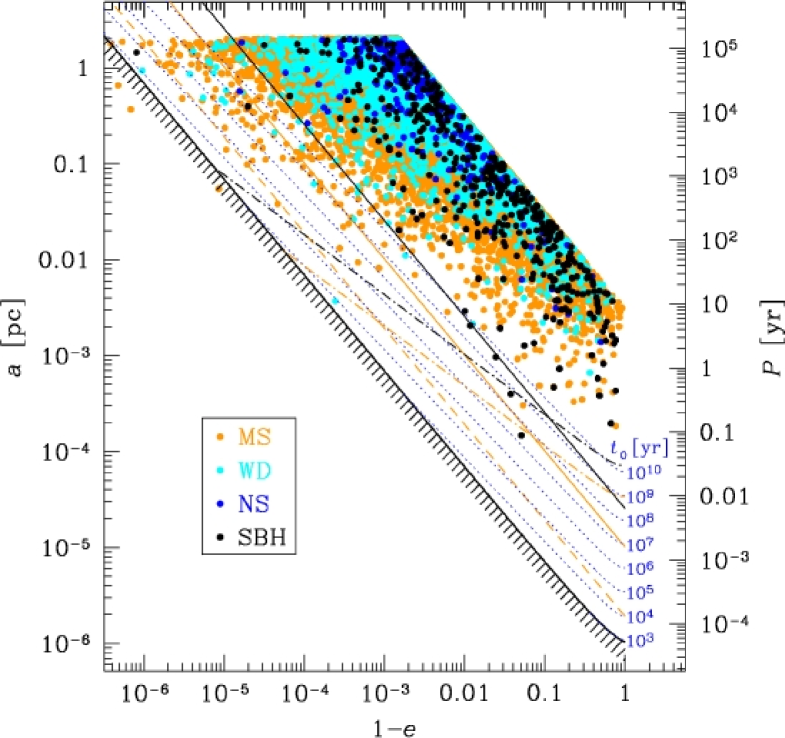
Figure 1: Realisation of the main model for the stellar cusp, with $1-e$ on the horizontal axis and the semi-major axis on the vertical axis (or period on the right vertical axis). Orange dots represent MS stars, cyan dots WDs, blue dots NSs, and black dots BHs, with numbers and slopes as described in the main model. The black line with hatching demarcates the last stable orbit. The dotted blue lines give the GW inspiraling time (Eq. 12) for the MS stars. The solid orange line indicate the ”burst region” for MS stars (with SNR=5). The solid black line line above it is for stellar BHs. The dashed orange line is the tidal disruption radius for MS stars. The orange dot-dashed line shows $t_{0}=(1-e)t_{r}$ for MS stars while the black one is for stellar BHs. Below these lines, depletion by GW inspiral should occur. The region with $P<1$ yr, where most bursting stars should be is almost entirely depleted due to the finite number effect.

A number of different possibilities were considered for the slopes and inner cut-offs of the respective stellar populations. The resulting GW burst rates for these models are summarized in table (1).

For our main model, we find that GW bursts are unlikely to be observed in the Galactic centre for MS stars ($\Gamma_{\rm MS}\sim 0.1\,{\rm yr^{-1}}$), for WDs ($\Gamma_{\rm WD}\sim 0.1\,{\rm yr^{-1}}$) and for NSs ($\Gamma_{\rm NS}\sim 0.004\,{\rm yr^{-1}}$). Our burst rate for MSs is much lower than the $\Gamma_{\rm MS}\sim 12\,{\rm yr^{-1}}$ rate estimated by RHBF06; the main reason for the difference is the cut-off due to collisions. Our rates for WDs and NSs are also lower than those found by RHBF06 (who estimated $\Gamma_{\rm WD}\sim 3\,{\rm yr^{-1}}$ and $\Gamma_{\rm NS}\sim 0.1\,{\rm yr^{-1}}$); here the difference is probably caused mainly by the different density profile, and the fact that the cusp runs out of stars at small radii from the MBH. On the other hand, we find a higher rate of BH bursts, ($\Gamma_{\rm BH}\sim 1\,{\rm yr^{-1}}$), which is the result of the steeper density profile we assumed, caused by mass-segregation (Freitag et al., 2006; Hopman & Alexander, 2006b). The inner radius for BHs was determined by GW inspiral in this case (§3.3.3).

The cumulative probability to detect more than a certain number of bursts per year can be determined with Monte Carlo sampling (§4). It consists of several factors, including the probability that in spite of the finite number effect a star has a very short period in a certain realisation. In this latter case there is a large number of correlated bursts, so that the distribution is not Poissonian. We show the results for the main model in Fig. (2). The average rates are in good agreement with our analytical model. Smaller differences are that for WDs and NSs, the Monte Carlo rates are slightly higher because of rare events excluded in the analytical model, while for BHs the rates are slightly lower, due to a small difference in the criterion for GW inspiral. From the figure it can be confirmed that the probability to observe even one single burst for MSs, WDs and NSs is negligible, but there is some chance to observe several GW bursts from BHs. The probability that the rate of observed BH bursts per year is exceeds 1 is $P(>1\,\,{\rm yr^{-1}})\approx 20\%$. For illustration purposes, we show in Fig (1) an example of a realisation of the main model.

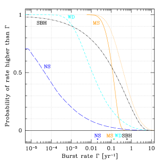
Figure 2: Distribution of burst rates for 40 000 Monte Carlo realisations. We plot the probability for the burst rate of each stellar species to be larger than a value $\Gamma$ as a function of $\Gamma$. Each cusp realisation consists of $N_{h}=3.4\times 10^{6}$ particles distributed around an MBH according to the parameters of the main model, such as illustrated in Fig. (1). Stars on plunge orbits or with $(1-e)t_{r}>t_{0}(r_{p},a)$ (see § 3.3.3) are discarded. We also remove MS stars with periapse distance smaller than the tidal disruption radius $r_{t}\simeq 2\times 10^{-6}\,$pc or semi-major axis smaller than the collision radius $r_{\rm coll}=3\times 10^{-3}\,$pc. The dotted line indicate the rate distribution for MS stars if there were no collisional depletion ($r_{\rm coll}=0$). The triangles above the horizontal axis indicate the rates averaged over all realisations. Notice that, except for MS stars, they are much higher than the median rates.

To probe the sensitivity of the GW burst rate to the assumptions, a number of other possibilities are considered explicitly. We stress that these models lack in realism; we consider them with the purpose of probing how sensitive our results are to the assumptions made.

First, consider the possibility that there is mass segregation, but an inner cut-off of only $a_{\rm min}=3\times 10^{-5}\,\mathrm{pc}$ for all stars (this is approximately where bursting sources become continuous sources, see eq. [5] and RHBF06). This increases the rate considerably for all species. The GW burst rate is plotted in Fig. (3). From this figure it can also be seen what the event rates for the main model are, by considering the appropriate cut-off for each species.

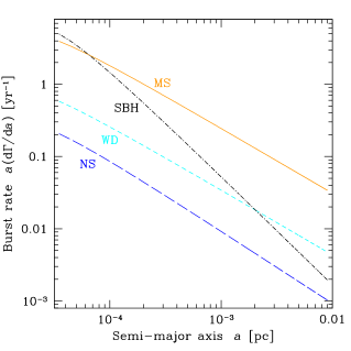
Figure 3: The rate $a{\rm d}\Gamma_{M}/{\rm d}a$ for the preferred model with $(\alpha_{\rm MS},\alpha_{\rm WD},\alpha_{\rm NS},\alpha_{\rm BH})=(1.4,1.4,1.5,2)$ and $(C_{\rm MS},C_{\rm WD},C_{\rm NS},C_{\rm BH})=(1,0.14,0.009,6\times 10^{-3})$. The required signal to noise ratio for detection was assumed to be $\rho=5$. The lines are extended for the case where there is no inner cut-off to the distribution function. In our main model, the rate does have an inner cut-off, see table (1).

Alternatively, we consider the case that there is an inner cut-off equal for all species to that of the main model, but that the slope is $\alpha_{M}=1.75$ for all species, as would be the case for a single mass population. We used a normalization $(C_{\rm MS}:C_{\rm WD}:C_{\rm NS}:C_{\rm BH})=(1:0.1:0.01:1\times 10^{-3})$ here. This example would present some realism if all stars are of similar mass and in particular if the typical mass of stellar BHs would be of the order $M_{\rm BH}\sim 1\,M_{\odot}$, or if the number of stellar BHs would be much smaller than assumed here (in the latter case the burst rate of the BHs would of course be lower). In this case, the GW burst rate would be dominated by WDs, with a rate of the order of $\Gamma_{\rm WD}\sim 4\,{\rm yr^{-1}}$. Interestingly, the cut-offs for this model are determined by different mechanism than for our main model (see table 1).

Finally, equation (8) was applied to model parameters similar to those assumed by RHBF06, i.e., without mass-segregation and with a fixed, very small inner cut-off. In this case an event rate is found that is more than an order of magnitude above that found by RHBF06. It is unclear what causes the discrepancy.

Model	Star	$m$	$C_{M}$	$\alpha_{M}$	$a_{\rm in}$	Reason for cut-off	$\Gamma_{M}$
		$[M_{\odot}]$			$[\,\mathrm{pc}]$		$[\,{\rm yr^{-1}}]$
Mass segregation, cut-off (main model)	MS	0.5	1.0	1.4	$3\times 10^{-3}$	Collisions	0.1
…………………………………	WD	0.6	0.14	1.4	$6\times 10^{-4}$	Finite number	0.09
…………………………………	NS	1.4	0.009	1.5	$2\times 10^{-3}$	Finite number	$4\times 10^{-3}$
…………………………………	SBH	10	$6\times 10^{-3}$	2.0	$3\times 10^{-4}$	GW inspiral	1.5
Mass segregation, no cut-off	MS	0.5	1.0	1.4	$3\times 10^{-5}$	-	6
…………………………………	WD	0.6	0.14	1.4	$3\times 10^{-5}$	-	0.8
…………………………………	NS	1.4	0.009	1.5	$3\times 10^{-5}$	-	0.3
…………………………………	SBH	10	$6\times 10^{-3}$	2.0	$3\times 10^{-5}$	-	5
No mass segregation, cut-off	MS	0.5	1.0	1.75	$3\times 10^{-3}$	Collisions	0.5
…………………………………	WD	0.6	0.1	1.75	$1\times 10^{-4}$	GW inspiral	4
…………………………………	NS	1.4	0.01	1.75	$5\times 10^{-4}$	Finite number	0.1
…………………………………	SBH	10	$1\times 10^{-3}$	1.75	$3\times 10^{-3}$	Finite number	$2\times 10^{-3}$
No mass segregation, no cut-off	MS	0.5	1.0	1.75	$3\times 10^{-5}$	-	280
…………………………………	WD	0.6	0.1	1.75	$3\times 10^{-5}$	-	42
…………………………………	NS	1.4	0.01	1.75	$3\times 10^{-5}$	-	5
…………………………………	SBH	10	$1\times 10^{-3}$	1.75	$3\times 10^{-5}$	-	0.7

Table 1: Event rates for a number of different stellar species and slopes. For all cases the required signal to noise ratio for detection was assumed to be $\rho=5$. The first four entries give the favored model, which accounts for mass-segregation according to the results by Hopman & Alexander (2006b), and has an inner cut-off of the cusp due to stellar collisions or finite number effects. The following four entries give the same model, but with equal inner cut-offs $r_{\rm in}=3\times 10^{-5}\,\mathrm{pc}$ for all stars. The next four entries are without mass-segregation, but with an inner cut-off; this could be appropriate if there are no SBHs (although they do appear in the table), in which case mass-segregation would be much less extreme. The last four entries also have the same inner cut-off, and an equal slope $\alpha=1.75$ as appropriate for a single mass cusp, similar to what was assumed by RHBF06.

6 Summary and discussion

When stars come very close ($r_{p}\lesssim 60r_{S}$, see Eq. 5) to the MBH in our Galactic centre, they emit a burst of GWs that could be observable by LISA (RHBF06). In this paper an analytical estimate for the burst rate is given. The estimate includes physics that was not considered by RHBF06, in particular mass-segregation and processes which determine the inner cut-off of the stellar distribution function. Mass-segregation mostly leads to different contributions from different species. However, since the event rate is dominated by stars very near the MBH (Eq. 8), the inner cut-of leads to a strong suppression of the GW burst rate. We find that only stellar BHs have a reasonable chance of being observed as bursting sources, with a rate of the order of $\Gamma\sim 1\,{\rm yr^{-1}}$ for signal to noise $\rho=5$.

The stellar distribution function in the inner $0.01\,\mathrm{pc}$ is not known in the Galactic centre, and the results presented here rely on theoretical estimates, rather than on observations. The role of collisions on the inner structure of the cusp is still poorly known, and if the inner cut-off would be considerably smaller than assumed here, the GW burst rate for MS stars grows substantially. Observation of a number of GW bursts from the Galactic centre would therefore have implications for our understanding of stellar dynamics near MBHs. The observation of a GW burst would probably allow one to constrain the masses of the system. In our models, we find that stellar BHs are the most likely candidates to be bursting sources. However, if the bursting source is a WD, then this would imply that either stellar BHs have masses much lower than $10M_{\odot}$, or that their number is much smaller than assumed here; in both cases the distribution of WDs would be steeper than we assumed, and our model with cut-off, but without mass-segregation, indicates that several WD bursts per year are then to be expected. Interestingly, similar conclusions would apply for inspiral sources (Hopman & Alexander, 2006b).

Using stellar dynamics simulations, Freitag (2003) suggested that, at any given time there are $\sim 1-3$ continuous GW sources at the Galactic centre (i.e., EMRIs), namely MS stars with a mass of $\sim 0.05-0.1\,M_{\odot}$ on orbits with $P\lesssim 3\times 10^{4}\,$s. This result would imply a burst rate much higher than estimated here. We note that a large population of low-mass MS stars would lead to a slightly higher burst rate because of the larger number of stars and the weaker depletion by GW emission. However, the EMRI rates obtained by Freitag (2003) seem to have been overestimated, due to the approximate treatment of the condition for GW-driven inspiral relying on a noisy particle-based estimate of the relaxation time. Furthermore, in that work, once it had reached the GW-dominated regime the possibility for a MS star to be destroyed by collisions was neglected.

We stress that a star on route to become an EMRI is unlikely to be a bursting source: the event rate at which EMRIs are created is of order $\Gamma_{\rm EMRI}\sim 0.1{\,\rm Myr^{-1}}$, while the time which a typical future EMRI spends at orbits with periods less than $1{\,\rm yr}$ is $t_{i}\sim 0.05{\,\rm Myr}$ (Hopman & Alexander, 2006b), implying that the probability of observing such a source in the GC is of order $\sim t_{i}\Gamma_{\rm EMRI}\sim 5\times 10^{-3}$. This confirms our assumption that the inner regions of the cusp are depleted in presence of GW energy losses (§3.3.3).

Bursts of GWs from stars passing close to extra-galactic MBHs are a potential source of noise for LISA . An estimate of the contribution to LISA ’s noise budget is out of the scope of this paper, and will be considered elsewhere.

RHBF06 also considered the possibility of observing GW bursts from the Virgo cluster, and estimated that only stellar BHs could be observed as bursting sources, with of the order of 3 bursts per year. We note that our higher rate of bursting BHs in the centre of our Galaxy than that found by RHBF06 does not imply that we also predict a higher rate of bursts from Virgo: for fixed signal to noise, a smaller periapse is required in Virgo, which in turn implies a larger inner cut-off of the density profile (see eq. 14). Taking this into account, we find that the bursting rate in Virgo is only of the order of $\sim 10^{-4}\,{\rm yr^{-1}}$ per galaxy, yielding a negligible rate for the Virgo cluster.

References

- Alexander (1999) Alexander T., 1999, ApJ, 527, 835
- Alexander (2005) Alexander T., 2005, Phys. Rep., 419, 65
- Alexander & Hopman (2003) Alexander T., Hopman C., 2003, ApJL, 590, L29
- Bahcall & Wolf (1976) Bahcall J. N., Wolf R. A., 1976, ApJ, 209, 214
- Bahcall & Wolf (1977) Bahcall J. N., Wolf R. A., 1977, ApJ, 216, 883
- Barack & Cutler (2004a) Barack L., Cutler C., 2004a, Phys. Rev. D., 70, 122002
- Barack & Cutler (2004b) Barack L., Cutler C., 2004b, Phys. Rev. D., 69, 082005
- Baumgardt et al. (2004a) Baumgardt H., Makino J., Ebisuzaki T., 2004a, ApJ, 613, 1133
- Baumgardt et al. (2004b) Baumgardt H., Makino J., Ebisuzaki T., 2004b, ApJ, 613, 1143
- Bender & Hils (1997) Bender P. L., Hils D., 1997, Classical and Quantum Gravity, 14, 1439
- Binney & Tremaine (1987) Binney J., Tremaine S., 1987, Galactic Dynamics. Princeton University Press, Princeton, NJ
- Chandrasekhar (1943) Chandrasekhar S., 1943, ApJ, 97, 255
- Cohn & Kulsrud (1978) Cohn H., Kulsrud R. M., 1978, ApJ, 226, 1087
- Eisenhauer et al. (2005) Eisenhauer F., et al., 2005, ApJ, 628, 246
- Figer et al. (2004) Figer D. F., Rich R. M., Kim S. S., Morris M., Serabyn E., 2004, ApJ, 601, 319
- Finn & Thorne (2000) Finn L. S., Thorne K. S., 2000, Phys. Rev. D., 62, 124021
- Frank & Rees (1976) Frank J., Rees M. J., 1976, MNRAS, 176, 633
- Freitag (2001) Freitag M., 2001, Classical and Quantum Gravity, 18, 4033
- Freitag (2003) Freitag M., 2003, ApJL, 583, L21
- Freitag et al. (2006) Freitag M., Amaro-Seoane P., Kalogera V., 2006, ApJ, 649, 91
- Freitag & Benz (2002) Freitag M., Benz W., 2002, A.A.P., 394, 345
- Freitag & Benz (2005) Freitag M., Benz W., 2005, MNRAS, pp 245–+
- Gair et al. (2004) Gair J. R., Barack L., Creighton T., Cutler C., Larson S. L., Phinney E. S., Vallisneri M., 2004, Classical and Quantum Gravity, 21, 1595
- Genzel et al. (2003) Genzel R., et al., 2003, ApJ, 594, 812
- Ghez et al. (2003) Ghez A. M., et al., 2003, ApJL, 586, L127
- Ghez et al. (2005) Ghez A. M., Salim S., Hornstein S. D., Tanner A., Lu J. R., Morris M., Becklin E. E., Duchêne G., 2005, ApJ, 620, 744
- Glampedakis (2005) Glampedakis K., 2005, Classical and Quantum Gravity, 22, 605
- Gould & Quillen (2003) Gould A., Quillen A. C., 2003, ApJ, 592, 935
- Hils & Bender (1995) Hils D., Bender P. L., 1995, ApJL, 445, L7
- Hopman (2006) Hopman C., 2006, astro-ph/0608460
- Hopman & Alexander (2005) Hopman C., Alexander T., 2005, ApJ, 629, 362
- Hopman & Alexander (2006a) Hopman C., Alexander T., 2006a, ApJ, 645, 1152
- Hopman & Alexander (2006b) Hopman C., Alexander T., 2006b, ApJL, 645, L133
- Ivanov (2002) Ivanov P. B., 2002, MNRAS, 336, 373
- Larson (2001) Larson S. L., Online Sensitivity Curve Generator, 2001, located at http://www.srl.caltech.edu/shane/sensitivity/; based on Larson, S. L., Hellings, R. W. & Hiscock, W. A., 2002, Phys. Rev. D, 66, 062001.
- Larson et al. (2000) Larson S. L., Hiscock W. A., Hellings, R. W., 2000, Phys. Rev. D, 62, 062001.
- Lightman & Shapiro (1977) Lightman A. P., Shapiro S. L., 1977, ApJ, 211, 244
- Lin & Tremaine (1980) Lin D. N. C., Tremaine S., 1980, ApJ, 242, 789
- Miralda-Escudé & Gould (2000) Miralda-Escudé J., Gould A., 2000, ApJ, 545, 847
- Mouawad et al. (2005) Mouawad N., Eckart A., Pfalzner S., Schödel R., Moultaka J., Spurzem R., 2005, Astronomische Nachrichten, 326, 83
- Murphy et al. (1991) Murphy B. W., Cohn H. N., Durisen R. H., 1991, ApJ, 370, 60
- Peebles (1972) Peebles P. J. E., 1972, ApJ, 178, 371
- Perets et al. (2006) Perets H. B., Hopman C., Alexander T., 2006, pre-print: astro-ph/0606443
- Peters (1964) Peters P. C., 1964, Physical Review, 136, 1224
- Preto et al. (2004) Preto M., Merritt D., Spurzem R., 2004, ApJL, 613, L109
- Rauch & Ingalls (1998) Rauch K. P., Ingalls B., 1998, MNRAS, 299, 1231
- Rauch & Tremaine (1996) Rauch K. P., Tremaine S., 1996, New Astronomy, 1, 149
- Rubbo et al. (2006) Rubbo L. J., Holley-Bockelmann K., Finn L. S., 2006, ApJL, 649, L25 (RHBF06)
- Schödel et al. (2002) Schödel R., et al., 2002, Nature, 419, 694
- Schödel et al. (2003) Schödel R., Ott T., Genzel R., Eckart A., Mouawad N., Alexander T. E., 2003, ApJ, 596, 1015
- Serabyn & Morris (1996) Serabyn E., Morris M., 1996, Nature, 382, 602
- Sigurdsson & Rees (1997) Sigurdsson S., Rees M. J., 1997, MNRAS, 284, 318