Long-term infrared variability of the UX Ori-type star SV Cep

Abstract

We investigate the long-term optical-infrared variability of SV Cep, and explain it in the context of an existing UX Ori (UXOR) model. A 25-month monitoring programme was completed with the Infrared Space Observatory in the 3.3–100 $\mu$m wavelength range. Following a careful data reduction, the infrared light curves were correlated with the variations of SV Cep in the V-band. A remarkable correlation was found between the optical and the far-infrared light curves. In the mid-infrared regime the amplitude of variations is lower, with a hint for a weak anti-correlation with the optical changes. In order to interpret the observations, we modelled the spectral energy distribution of SV Cep assuming a self-shadowed disc with a puffed-up inner rim, using a 2-dimensional radiative transfer code. We found that modifying the height of the inner rim, the wavelength-dependence of the long-term optical-infrared variations is well reproduced, except the mid-infrared domain. The origin of variation of the rim height might be fluctuation in the accretion rate in the outer disc. In order to model the mid-infrared behaviour we tested to add an optically thin envelope to the system, but this model failed to explain the far-infrared variability. Infrared variability is a powerful tool to discriminate between models of the circumstellar environment. The proposed mechanism of variable rim height may not be restricted to UXOR stars, but might be a general characteristic of intermediate-mass young stars.

1 Introduction

UX Orionis stars are intermediate mass pre-main sequence objects defined by the ’UXOR phenomenon’: short (days to weeks) eclipse-like dimming at optical wavelengths. Earlier explanations of the phenomenon invoked a large number of protocometary clouds or cometary bodies Grady et al. (2000), or assumed that UX Ori objects are surrounded by an almost edge-on protoplanetary disc, where hydrodynamic fluctuations of the disc surface can cause dust filaments passing in front of the star Bertout (2000). A more recent model of Dullemond et al. Dullemond (2003) proposes that UX Ori stars harbour self-shadowed discs (the type of Group II in the classification scheme of Meeus et al. 2001), where a puffed-up rim at the inner edge of the disc casts shadow over the whole disc. Small hydrodynamical fluctuations in the puffed-up rim along the line-of-sight may cause the extinction events seen in UXORs.

The fact that UXORs may also exhibit long-term variability received much less attention so far in the literature. Rostopchina et al. Rostopchina (2000) reported that brightness variations on a timescale of several years with an amplitude of 0.2–1.0 mag can be a characteristic of the UXOR class. They conclude that a possible reason of these brightness variations can be changes of large scale structures in the protoplanetary discs around these stars.

It is an important test for the self-shadowed disc hypothesis (and in general for any UXOR model) to check whether the observed long-term variations could be interpreted in the framework of the model. One possibility would be to assume that some effects in the inner rim (e.g. weak accretion) change the rim’s height along a significant fraction of its perimeter (rather than along the line-of-sight only), thus the eclipses may last longer. Another hypothesis is that the disc is not completely self-shadowed but has a moderately flared outer part (tenuous enough to ensure that the star is still visible), and in these outer regions dense filaments pass in front of the star. Due to the larger Keplerian times, these eclipses in the outer disc last significantly longer than the normal UXOR events.

A powerful tool to discriminate between such possibilities is looking for variability in the thermal infrared emission of the circumstellar disc. If the optical changes are due to line-of-sight effects then no infrared variability is expected, since the total irradiation of the disc by the star, and consequently the disc’s total integrated infrared emission, is constant. But if a considerable re-structuring of the inner rim occurs, it could affect the illumination of the disc by the star, leading to changes in the infrared emission, too.

In this paper we report on the results of an infrared monitoring programme of the UX Orionis-type star SV Cephei. SV Cep is an A0-B9 star (Rostopchina et al. 2000) with an age of $4\cdot 10^{6}$ yrs (Natta et al. 1997). Its distance is estimated to be 700 pc, with some uncertainty Kun et al. (2000). The brightness of SV Cep varies on a long timescale ($\sim$4000 days) between 10.5 and 11.5 mag in the V-band, with some hints for a quasi-periodic behaviour (Rostopchina et al. 2000). The infrared monitoring programme was carried out with the Infrared Space Observatory (ISO) for 25 months. It is important that near-simultaneous optical data were available for the same period in the literature.

In Sect. 2 we summarize the ISO observations and data reduction. We present a new algorithm for the evaluation of the ISOPHOT photometry, which was successfully used to reduce the relative uncertainties within the light curves. In Sect. 3 we present the results, then in Sect. 4 we model the light variations assuming a self-shadowed disc with a puffed-up inner rim and a tenuous, moderately flared outer part, using a radiative transfer code. Section 5 provides a summary of the work.

2 Observations and data reduction

2.1 Observations

SV Cep was observed with ISOPHOT Lemke et al. (1996), the photometer on-board the Infrared Space Observatory, between 1996 and 1998. The measurements were part of a monitoring programme dedicated to investigate the infrared variability of UXORs. Observations were performed at 12 wavelengths between 3.3 and 100 $\mu$m, at 13-19 epochs depending on the wavelength. The filters belong to three ISOPHOT subsystems: the P1 detector (3.3–15 $\mu$m), the P2 detector (20 and 25 $\mu$m), and the P3 detector (60 and 100 $\mu$m). Observations were performed using the Astronomical Observing Template PHT03. The source (’ON’) and the background (’OFF’) positions were measured separately, always starting with the ’OFF’ position. Measurements with all filters belonging to a specific detector (P1, P2 or P3) were performed first, then a calibration measurement on the on-board Fine Calibration Source (FCS) was obtained using the last filter. The log of the monitoring observations is presented in Tab. 1.

In addition, two 3x3 mini-rasters at 150 and 200 $\mu$m with the ISOPHOT-C200 camera (ISO_id: 56201201), as well as a 2–12 $\mu$m spectrophotometric measurement with the ISOPHOT-S subinstrument (ISO_id: 56201203) were obtained on May 31, 1997.

2.2 Standard data processing

We processed all observations using the Phot Interactive Analysis V10.0 (PIA) Gabriel et al. (1997) following the standard data reduction scheme. First, non-linearity correction was performed on the integration ramps, then the two-threshold deglitching method was applied to remove cosmic particle hits. With a first order polinomial fit to each ramp, we evaluated the signal value and reached the Signal per Ramp Data (SRD) level. Here reset interval correction was performed, dark current was subtracted and cosmic particle hits were again checked. We took the average of the signal values to reach the next data processing level, which is called Signal per Chopper Plateau (SCP). Since the signal in many cases did not stabilize, we averaged only the stable part of the measurement when possible. The final step was the power calibration, which could be carried out by adopting either the actual or the default responsivity value. The actual responsivity is derived from the FCS measurement, while the default one is a tabulated value, computed from data over the whole ISO mission. We decided to use default responsivity for the P1 and P2 detectors, and actual responsivity for filters belonging to the P3 detector.

According to the ISOPHOT Handbook (Laureijs et al. 2003), the typical absolute photometric accuracy of the type of OFF/ON measurements is 40%, 15%, and 15% for the P1, P2, and P3 detectors, respectively, in the brightness range of SV Cep. Due to the nearly identical instrument setup the relative photometric uncertainties within the light curve, however, may be lower than these values. In order to have an independent estimate of the relative flux uncertainties, COBE/DIRBE data were analysed. We compared the temporal brightness variations of the ISOPHOT background measurements with the corresponding DIRBE data extracted for the same coordinates and solar elongations (see Fig. 1a). Though the DIRBE measurements are presented as surface brightness values in [MJy/sr] and the ISOPHOT data are in flux density units of [Jy] the ratio between the two datasets depends only on the beam size of ISOPHOT and should be constant. Thus the standard deviation of this ratio around an average value can be adopted as the relative photometric error of the normalized light curve. The resulting values are 22%, 13%, and 10% for the P1, P2, and P3 detectors, respectively.

Figure 1: Comparison of the standard and the new data processing schemes at 12 $\mu$m. The solid line is a normalized curve interpolated among DIRBE measurements. Filled dots are the normalized ISOPHOT measurements: a) reduced with the standard method and b) reduced with our new data processing scheme. The second last ISOPHOT measurement on the upper figure is too high, and falls out of the figure range.

The far-infrared mini-rasters at $150$ and $200\,\mu$m were processed with PIA in the standard way up to the calibrated map level (for calibration the FCS measurements were used). Flux extraction was performed by fitting the measured ISOPHOT point-spread function to the brightness distribution in the map. The ISOPHOT-S observation was reduced following the processing scheme described by Ábrahám & Kun phts (2004), which checks for memory effects and possible off-centre positioning of the source, subtracts an estimated background spectrum, and adopts realistic error bars.

2.3 A new processing scheme

When looking for variability, usually the highest possible photometric accuracy is needed. We developed an independent new processing scheme for the ISOPHOT photometry, which takes into account that in a monitoring programme a uniform observing strategy (filter sequence, heating power of the FCS which determines its optical emission, etc.) is adopted at each epoch. This similarity of the observing sequences helps to handle the detector transients in a better way, and achieve a higher relative accuracy. The basic idea is the following: due to the detector transients the signals are usually not stabilized during the measurement time, but because of the identical observing strategy and illumination history, the shapes of the transient curves are self-similar on the different days. In our new data reduction method we do not attempt to determine ’stabilized signal level’ (e.g. by extrapolating the transient curves, or by averaging its stable-looking part), but measure relative flux changes from one day to the other via direct comparison of the complete unstabilized transient curves.

As outlined in Fig. 2, first we compare the FCS signals, and – since they correspond to the same optical power – determine the responsivity difference between the two epochs. In practice, this comparison is done by computing a scaling factor between the – usually unstabilized – signal sequences at the SRD level. This factor is applied also on the sky measurements, since they are also affected by responsivity changes. Then the ratio of the corrected sky signals of the two days is computed, which should now reflect true brightness variations only. This way a relative light curve can be built up with respect to a reference epoch. Absolute fluxes can be obtained by multiplying this normalized curve with the calibrated flux value of the reference day, as determined in Sect. 2.2.

Figure 2: Determining relative signal ratios in the case of two ’ON’ measurements at 100 $\mu$m, following the principles of our new processing scheme (Sect. 2.3). In the first step the FCS signals are scaled together, in order to correct for responsivity differences, then the ratio of the corrected SV Cep signal curves is computed. The accuracy of the relative flux difference is a few percent.

There were monitoring sequences, however, when the FCS heating power was not kept constant for each epoch. For such cases we propose two solutions. In Method A, which can be applied only for background measurements, we divide the sequence into as many groups as many different heating power values exist in the sequence. Then we choose a reference day in each group and build up the normalized light curves of these groups separately, as described above. Extracting COBE/DIRBE data for the sky positions and solar elongations of the ISOPHOT background measurements, for each group the mean ISOPHOT/DIRBE ratio is computed. Since this ratio should be the same for all groups, we divide the normalized light curve of a group by the ratio between the mean ISOPHOT/DIRBE value of the group and that of the reference group. In the final step we merge the groups to create the final light curve of the whole sequence.

In Method B, which can also be applied on source measurements, we take into account that the optical power of the lamp differs between the two epochs, and scale the levels of the FCS signal curves according to this power difference. The optical powers are specified in the FCS calibration files. After this scaling the FCS transient curves can be compared as before in order to determine the responsivity difference. The only disadvantage of this method is that the shapes of FCS transient curves of different heating powers may be less similar.

2.4 Application of the new method on SV Cep

The new processing scheme produces separate OFF and ON light curves, whose difference shows the temporal variability of the object. As a reference day for the final normalized light curves of SV Cep we chose January 24, 1997, when most measurements showed particular stability. We started with the rather homogeneous 100 $\mu$m sequence (14 epochs, see Tab. 1), where each FCS measurement was carried out with the 100 $\mu$m filter, and not more than 3 different FCS heating powers were used. We applied Method A on the background measurements, including a relatively large correction on the first day (February 10, 1996) when the ISOPHOT/DIRBE ratio was significantly higher than its average value (by more than 3$\sigma$), thus we scaled down the ISOPHOT OFF signal by this ratio. Since at 100 $\mu$m the ON and OFF signal levels were comparable and the same FCS heating power was used for both source and background measurements, we decided to apply the correction factors derived for background measurements on the source measurements, too. At 60 $\mu$m the observational sequence was less homogeneous, since the FCS calibration was carried out either with the 60 $\mu$m or the 100 $\mu$m filter, and different heating powers were used. Thus we had to apply Method B in this case, and again a noticeable correction was necessary at the first epoch. At 20 and 25 $\mu$m (P2 detector), and at shorter wavelengths (P1 detector) we always used Method B.

The relative photometric uncertainties were again evaluated via comparison with DIRBE background measurements (see Fig. 1$b$ for the 12 $\mu$m filter). The figure shows that our new data processing scheme produces significantly lower relative photometric errors compared to the standard method. The errors of the final ON-OFF differential photometry are typically 14–15 % at 60 and 100 $\mu$m; 14–15 % at 20 and 25 $\mu$m; and are about 8-9 % for the P1 filters (the latter was computed at 12$\mu$m and adopted for the other P1 filters, too).

Date	ISO_id	$\lambda$	Aperture	FCS heat. pow.
	OFF / ON	[$\mu$m]	[$\arcsec$]	OFF / ON [mW]
10-Feb-1996	08502135 / 36	3.3,3.6,4.8,7.3,10.0,12.0,12.8,15.0	18	7.37485 / 4.55433
	08502135 / 36	20,25	52	1.50183 / 1.86813
	08502135 / 36	60,100	120	0.58608 / 0.68376
28-May-1996	19302325 / 26	3.3,3.6,4.8,7.3,10.0,12.0,12.8,15.0	18	7.98535 / 5.88523
	19302325 / 26	20,25	52	1.50183 / 2.24664
	19302325 / 26	60,100	120	0.41514 / 0.41514
28-Jul-1996	25500127 / 28	3.3,3.6,4.8,7.3,10.0,12.0,12.8,15.0	18	8.00977 / 5.88523
	25500127 / 28	20,25	52	1.50183 / 2.24664
	25500127 / 28	60,100	120	0.41514 / 0.41514
08-Oct-1996	32601431 / 32	3.3,3.6,4.8,7.3,10.0,12.0,12.8,15.0	18	8.00977 / 5.88523
	32601431 / 32	20,25	52	1.50183 / 2.24664
	32601431 / 32	60,100	120	0.41514 / 0.41514
03-Dec-1996	38300901 / 02	3.6,12.0	18	8.00977 / 5.88523
	38300901 / 02	20,25	52	1.40415 / 1.79487
	38300901 / 02	60	120	0.59829 / 0.70818
31-Dec-1996	41100637 / 38	3.6,12.0	18	8.00977 / 5.88523
	41100637 / 38	20,25	52	1.40415 / 1.79487
	41100637 / 38	60	120	0.59829 / 0.70818
31-Dec-1996	41100733 / 34	3.3,3.6,4.8,7.3,10.0,12.0,12.8,15.0	18	8.00977 / 5.88523
	41100733 / 34	20,25	52	1.40415 / 2.21001
	41100733 / 34	60,100	120	0.35409 / 0.35409
21-Jan-1997	43101241 / 42	3.6,12.0	18	8.00977 / 5.88523
	43101241 / 42	20,25	52	1.40415 / 1.79487
	43101241 / 42	60	120	0.59829 / 0.70818
24-Jan-1997	43501229 / 30	3.3,3.6,4.8,7.3,10.0,12.0,12.8,15.0	18	8.00977 / 5.88523
	43501229 / 30	20,25	52	1.40415 / 2.21001
	43501229 / 30	60,100	120	0.35409 / 0.35409
07-Feb-1997	44901743 / 44	3.3,3.6,4.8,7.3,10.0,12.0,12.8,15.0	18	8.00977 / 5.88523
	44901743 / 44	20,25	52	1.40415 / 2.21001
	44901743 / 44	60,100	120	0.35409 / 0.35409
31-May-1997	56200647 / 48	3.3,3.6,4.8,7.3,10.0,12.0,12.8,15.0	18	8.00977 / 5.90965
	56200647 / 48	20,25	52	1.40415 / 2.21001
	56200647 / 48	60,100	120	0.35409 / 0.35409
31-May-1997	56200845 / 46	3.6,12.0	18	8.00977 / 5.90965
	56200845 / 46	20,25	52	1.40415 / 1.79487
	56200845 / 46	60	120	0.59829 / 0.70818
31-May-1997	56201204 / 05	3.3,3.6,4.8,7.3,10.0,12.0,12.8,15.0	18	8.00977 / 5.90965
	56201204 / 05	20,25	52	1.40415 / 2.21001
	56201204 / 05	60,100	120	0.35409 / 0.35409
21-Jun-1997	58302203 / 04	3.3,3.6,4.8,7.3,10.0,12.0,12.8,15.0	18	8.00977 / 5.90965
	58302203 / 04	20,25	52	1.40415 / 2.21001
	58302203 / 04	60,100	120	0.35409 / 0.35409
26-Sep-1997	68100205 / 06	3.3,3.6,4.8,7.3,10.0,12.0,12.8,15.0	18	8.00977 / 5.90965
	68100205 / 06	20,25	52	1.40415 / 2.21001
	68100205 / 06	60,100	120	0.35409 / 0.35409
05-Dec-1997	75100107 / 08	3.3,3.6,4.8,7.3,10.0,12.0,12.8,15.0	18	8.00977 / 5.90965
	75100107 / 08	20,25	52	1.40415 / 2.21001
	75100107 / 08	60,100	120	0.35409 / 0.35409
21-Dec-1997	76700951 / 52	3.3,3.6,4.8,7.3,10.0,12.0,12.8,15.0	18	8.00977 / 5.90965
	76700951 / 52	20,25	52	1.40415 / 2.21001
	76700951 / 52	60,100	120	0.35409 / 0.35409
11-Mar-1998	84604849 / 50	3.6,12.0	18	8.00977 / 5.90965
	84604849 / 50	20,25	52	1.40415 / 1.79487
	84604849 / 50	60	120	0.59829 / 0.70818
29-Mar-1998	86500853 / 54	3.3,3.6,4.8,7.3,10.0,12.0,12.8,15.0	18	8.00977 / 5.90965
	86500853 / 54	20,25	52	1.40415 / 2.21001
	86500853 / 54	60,100	120	0.35409 / 0.35409

Table 1: Log of ISOPHOT observations.

Date	3.3 $\mu$m	3.6 $\mu$m	4.8 $\mu$m	7.3 $\mu$m	10.0 $\mu$m	12.0 $\mu$m
10-Feb-1996	0.524$\pm$0.036	0.458$\pm$0.092	0.470$\pm$0.094	0.711$\pm$0.142	4.697$\pm$0.939	3.704$\pm$0.741
28-May-1996	0.900$\pm$0.062	0.645$\pm$0.129	0.562$\pm$0.112	0.819$\pm$0.164	5.864$\pm$1.173	4.621$\pm$0.924
28-Jul-1996	0.711$\pm$0.049	0.664$\pm$0.133	0.627$\pm$0.125	0.855$\pm$0.171	5.801$\pm$1.160	4.579$\pm$0.916
8-Okt-1996	0.631$\pm$0.044	0.491$\pm$0.098	0.506$\pm$0.101	0.788$\pm$0.158	5.954$\pm$1.191	5.059$\pm$1.012
3-Dec-1996	-	0.493$\pm$0.099	-	-	-	5.147$\pm$1.029
31-Dec-1996	0.758$\pm$0.052	0.643$\pm$0.129	0.663$\pm$0.133	1.009$\pm$0.202	6.458$\pm$1.292	4.713$\pm$0.943
31-Dec-1996	-	0.553$\pm$0.111	-	-	-	5.130$\pm$1.026
21-Jan-1997	-	0.546$\pm$0.109	-	-	-	5.147$\pm$1.029
24-Jan-1997	0.659$\pm$0.046	0.610$\pm$0.122	0.633$\pm$0.127	1.000$\pm$0.200	7.068$\pm$1.414	5.144$\pm$1.029
7-Feb-1997	0.714$\pm$0.049	0.617$\pm$0.123	0.659$\pm$0.132	0.959$\pm$0.192	7.170$\pm$1.434	5.162$\pm$1.032
31-May-1997	-	0.671$\pm$0.134	-	-	-	4.319$\pm$0.864
31-May-1997	-	0.596$\pm$0.119	-	-	-	4.842$\pm$0.968
31-May-1997	0.774$\pm$0.054	0.648$\pm$0.130	0.614$\pm$0.123	0.902$\pm$0.180	6.491$\pm$1.298	4.987$\pm$0.997
21-Jun-1997	0.752$\pm$0.052	0.656$\pm$0.131	0.635$\pm$0.127	0.915$\pm$0.183	6.558$\pm$1.312	4.974$\pm$0.995
26-Sep-1997	0.653$\pm$0.045	0.631$\pm$0.126	0.638$\pm$0.128	0.871$\pm$0.174	6.053$\pm$1.211	4.826$\pm$0.965
5-Dec-1997	0.648$\pm$0.045	0.553$\pm$0.111	0.544$\pm$0.109	0.932$\pm$0.186	5.504$\pm$1.101	4.629$\pm$0.926
21-Dec-1997	0.660$\pm$0.046	0.556$\pm$0.111	0.583$\pm$0.117	0.868$\pm$0.174	6.575$\pm$1.315	5.078$\pm$1.016
11-Mar-1998	-	0.543$\pm$0.109	-	-	-	4.453$\pm$0.891
29-Mar-1998	0.562$\pm$0.039	0.525$\pm$0.105	0.484$\pm$0.097	0.757$\pm$0.151	5.758$\pm$1.152	4.930$\pm$0.986
Date	12.8 $\mu$m	15 $\mu$m	20 $\mu$m	25 $\mu$m	60$\mu$m	100 $\mu$m
10-Feb-1996	3.078$\pm$0.616	1.795$\pm$0.359	6.961$\pm$0.950	4.067$\pm$0.790	3.047$\pm$0.876	1.853$\pm$0.532
28-May-1996	3.805$\pm$0.761	2.149$\pm$0.430	7.570$\pm$1.102	3.846$\pm$0.658	1.941$\pm$0.471	1.541$\pm$0.374
28-Jul-1996	4.227$\pm$0.845	2.544$\pm$0.509	7.815$\pm$1.140	4.270$\pm$0.743	1.856$\pm$0.404	1.391$\pm$0.302
8-Okt-1996	4.030$\pm$0.806	1.907$\pm$0.381	7.699$\pm$1.102	3.972$\pm$0.641	1.701$\pm$0.375	1.316$\pm$0.290
3-Dec-1996	-	-	-	4.138$\pm$0.684	1.954$\pm$0.456	-
31-Dec-1996	4.311$\pm$0.862	2.648$\pm$0.530	7.471$\pm$1.068	3.947$\pm$0.639	2.116$\pm$0.521	1.091$\pm$0.255
31-Dec-1996	-	-	-	4.229$\pm$0.714	1.804$\pm$0.429	-
21-Jan-1997	-	-	-	3.789$\pm$0.609	1.658$\pm$0.402	-
24-Jan-1997	4.654$\pm$0.931	2.587$\pm$0.517	7.463$\pm$1.072	3.886$\pm$0.648	2.091$\pm$0.495	1.417$\pm$0.350
7-Feb-1997	4.694$\pm$0.939	2.597$\pm$0.519	7.582$\pm$1.110	4.247$\pm$0.731	1.799$\pm$0.406	1.496$\pm$0.356
31-May-1997	-	-	-	4.344$\pm$0.738	1.846$\pm$0.404	0.797$\pm$0.193
31-May-1997	-	-	-	3.894$\pm$0.648	1.740$\pm$0.381	-
31-May-1997	4.406$\pm$0.881	2.476$\pm$0.495	7.535$\pm$1.092	4.157$\pm$0.700	1.667$\pm$0.350	1.130$\pm$0.267
21-Jun-1997	4.498$\pm$0.900	2.466$\pm$0.493	7.384$\pm$1.042	4.108$\pm$0.688	1.543$\pm$0.325	1.074$\pm$0.253
26-Sep-1997	4.266$\pm$0.853	2.575$\pm$0.515	7.451$\pm$1.040	4.136$\pm$0.719	1.767$\pm$0.366	0.976$\pm$0.221
5-Dec-1997	3.950$\pm$0.790	2.494$\pm$0.499	7.124$\pm$0.970	3.561$\pm$0.560	1.607$\pm$0.348	1.211$\pm$0.255
21-Dec-1997	4.320$\pm$0.864	2.503$\pm$0.501	6.782$\pm$0.890	3.007$\pm$0.449	1.685$\pm$0.371	0.968$\pm$0.204
11-Mar-1998	-	-	-	3.806$\pm$0.630	1.325$\pm$0.263	-
29-Mar-1998	3.986$\pm$0.797	1.974$\pm$0.395	7.563$\pm$1.118	4.005$\pm$0.682	1.644$\pm$0.342	1.241$\pm$0.263

Table 2: Colour corrected flux densities of SV Cep in Jy. The quoted errors are the relative uncertainties of our new data processing scheme. The absolute flux errors from the standard method are higher by a factor of 2.5 for the P1 filters, 1.3 for the P2 filters and 2.5 for the P3 filters.

3 Results

The resulting flux density values for all 19 epochs are presented in Tab. 2. The far-infrared flux densities on May 31, 1997 (not included in the table) were the following: 0.664$\pm$0.186 Jy at 150 $\mu$m, and 0.498$\pm$0.075 Jy at 200 $\mu$m. All flux values are colour corrected. Colour correction factors were determined by convolving the ISOPHOT filter profiles with the shape of the spectral energy distribution (SED) in an iterative way. Since the general shape of the SED did not change considerably over the monitoring period, we computed correction factors for one particular day (May 31, 1997, see below) and used these values for all other epochs. The quoted uncertainties in Tab. 2 correspond to the relative photometric errors derived from the new processing scheme; the absolute photometric uncertainties are the higher values given in Sect. 2.2.

3.1 Spectral energy distribution

Before investigating the infrared variability, we constructed and studied the SED of SV Cep. Since the star is variable, we chose a single epoch, May 31, 1997, when a large number of ISOPHOT measurements were obtained (including far-infrared photometry at 150 and 200 $\mu$m as well as mid-infrared spectrophotometry), and constructed an SED for this reference epoch. Figure 3 shows the resulting SED. The 3.6–100 $\mu$m data were supplemented by optical UBVRI data, taken from Rostopchina et al. Rostopchina (2000) and interpolated for the reference epoch, as well as by a ground based millimeter-wave measurement Natta et al. (1997). The zero magnitude fluxes of the optical bands are taken from Bessel et al. (1979).

At wavelengths shorter than 1 $\mu$m the SED is dominated by the stellar component (Fig. 3). Between 2 and 8 $\mu$m a near-infrared bump can be seen, which is typical for many Herbig Ae stars Dullemond et al. (2001). Around 10 $\mu$m a strong silicate emission feature is present and probably the same silicate grains are responsible for the local peak at 20 $\mu$m. The continuum of the SED is approximately flat (in ${\nu}F_{\nu}$) below 25 $\mu$m, and decreases towards longer wavelengths approximately as F${}_{\nu}\propto\lambda^{-1.1}$. The fact that this slope is shallower than a Rayleigh-Jeans tail suggests the existence of cold, optically thin components at the outer part of the disc. In the submillimeter-wave region the shallower slope of the SED can be the consequence of presence of big grains settled to the disk midplane which radiate at these wavelengths.

Figure 3: SED of SV Cep. Flux uncertainties are usually smaller than the symbol size. No correction for interstellar reddening was performed.

3.2 Optical-infrared light curves

In Fig. 4 we plotted the light curves of SV Cep at four representative infrared wavelengths, as well as in the V-band. Infrared flux values are taken from Tab. 2; the V-band magnitudes are from Rostopchina et al. (2000).

In the V-band clear variability can be seen. It is not surprising, that the brightness of SV Cep changes on a time-scale of days to weeks, which is typical for UXORs, but the brightness varies also on a time-scale of hundred days. The peak-to-peak amplitude of the long-term flux variation of SV Cep is about 60%. At the beginning of the monitoring period, in 1996, SV Cep was in a bright state, then its brightness decreased steadily within the next 250 days. At the beginning of 1997 there was a local maximum, followed by a shallow decline in brightness. At the end of 1997 the direction of the brightness variation changed and SV Cep began to brighten again.

We can also recognize variability, exceeding the formal flux uncertainties, at 3.6 $\mu$m. The peak-to-peak flux variation is somewhat smaller than in the V-band. The flux increased during the first 200 days, then, except for a local minimum at the end of 1996, the brightness remained constant, within the errors, until the end of 1997. Then the flux slowly decreased until the last measured point. At 12 $\mu$m the peak-to-peak variability is even smaller than at 3.6 $\mu$m. The brightness slowly incresed during the first 450 days, then decreased with a similar pace. The light curves at the other six wavelengths from 3.3 to 15 $\mu$m (not shown) behave similar to the 3.6 and 12 $\mu$m results, but the amplitude of the variability decreases from 3.3 to 15 $\mu$m. The flux of SV Cep was almost constant at 20 and 25 $\mu$m over the observed 25 months, compared to the measurement uncertainties.

At 100 $\mu$m clear variability can be recognized, with a peak-to-peak change of about a factor of 2. The brightness decreased during the first 800 days, except for a local maximum at the beginning of 1997. From the beginning of 1998 the flux at 100 $\mu$m began to increase slowly. The shape of the light curve at 60 $\mu$m is very similar to that at 100 $\mu$m.

Figure 4: Light curves of SV Cep at four representative infrared wavelengths, as well as in the V-band. Infrared flux values are taken from Tab. 2; the V-band magnitudes are from Rostopchina et al. (2001). The plotted error bars correspond to the relative photometric uncertainties.

3.3 Correlations

Figure 5: Correlation diagrams between the optical and infrared light variations. All light curves are normalized for the reference day of May 31, 1997. Dotted lines are linear fits to the observations; dashed lines show the same for synthetic light curves obtained from modelling (Sect. 4).

In order to investigate the relationships between the optical and infrared data sets, we interpolated the V-band light curve for the epochs of the ISOPHOT observations. Then infrared data from Tab. 2 were plotted against the interpolated V-band fluxes (Fig. 5) at the same four wavelengths as in Fig. 4.

At 100 $\mu$m a clear correlation can be seen between the optical and the infrared flux values. The Pearson’s correlation coefficient is 0.88, which indicates a significant linear trend in the data distribution. A similar behaviour can be observed at 60 $\mu$m (not plotted). At 25 $\mu$m, and also at 20 $\mu$m (not shown), the correlation with the V-band disappears, due to the fact, that at these wavelengths SV Cep does not exhibit any significant variations (Fig. 4). The 3.6 $\mu$m and 12 $\mu$m correlation plots might indicate a weak anti-correlation with the V-band fluxes (Pearson’s correlation coefficients are -0.55 and -0.40, respectively). The significance of this anti-correlation mainly relies on the reliability of the photometric points at the very first epoch, whose calibration was not straightforward (see Sect. 2.4). However, simultaneous observations with the SWS instrument (the short-wavelength spectrometer on-board ISO) at 2.63 and 3.6$\mu$m seem to support the observed anti-correlation at mid-infrared wavelengths.

4 Discussion

4.1 Variability: a new tool to explore circumstellar structure

A number of numerical codes are available, which can model the SED of a young stellar object by assuming a certain circumstellar geometry (e.g. flat/flared disc, envelope) and performing radiative transfer calculations (e.g. Dullemond et al. Dullemond06 (2006) and references therein). In many cases, however, the model results are not unique: the SED can be fitted by assuming different circumstellar structures. One possibility to resolve this ambiguity is high spatial resolution imaging. Another way – which was first proposed by Chiang & Goldreich cg97 (1997) and which will be explored in this section – is to make predictions for possible flux variations in the different competing models and confront the synthetic light curves with the observations. In practice it is a three-step procedure:

Modelling the SED at one selected epoch. The abovementioned stationary models can be used to fit the SED at a selected epoch, in order to take a snapshot of the circumstellar structure. The best fitting model specifies, for any given wavelength, (i) which component of the circumstellar structure (e.g. puffed-up inner rim, disc atmosphere, midplane) dominates the infrared radiation in that part of the spectrum; and (ii) whether the emitting region is optically thin or optically thick for incident starlight. This information will be essential to model variability.

Tuning model setup parameters. The infrared emission of Young Stellar Objects (YSOs) can vary in time when the illumination of the circumstellar matter by the central source is not constant. Disc illumination can change if (1) the luminosity of the star varies (e.g. time-variable accretion onto the star; examples are the eruptive FU Ori- or EX Lup-type young stars); or (2) the circumstellar geometry is re-structured, modifying the illumination pattern on the disc (e.g. the scale height of the puffed-up inner rim – which casts a shadow on the outer disc – is not stable). These changes can be modelled by tuning the corresponding stellar/geometrical parameters in the setup of the stationary model of the circumstellar environment (i.e. luminosity of the central star or scale heights of the disc). The resulting SED can be compared with the one of the selected epoch, in order to predict the observable consequences of a changing stellar luminosity or circumstellar structure.

Timescales. The infrared emission does not react immediately to a change of illumination. The timescale depends on the radial distance of the emitting region from the centre and on its optical depth for the incident light. Optically thin disc surface layer or optically thick disc interior react to a change of illumination on completely different timescales, as computed by Chiang & Goldreich cg97 (1997). New time-dependent codes would be necessary to compute the timescales related to the changes of illumination for each wavelength correctly. However, as a first attempt, one can often assume that emission from an optically thin region (e.g. puffed-up rim, disc atmosphere) reacts instantaneously to the change of illumination, while the emission of optically thick components is practically constant on the timescales of the monitoring programme ($\sim$years). With these assumptions one can predict how the infrared emission would react, as a function of time, on variations of the illumination of the disc. The predictions can be compared with the measured infrared light curves. Significant discrepancies may reveal that the model assumptions on the circumstellar structure have to be modified in order to reach a closer match to reality.

4.2 Modelling of SV Cep

4.2.1 Disc model

Figure 6: SED of SV Cep. The measured data points are corrected for an interstellar reddening of 0.74^m. Overplotted is the best fitted disc model.

Modelling the SED. In Sect. 1 we asked the question whether the observed long-term variability of SV Cep could be interpreted in the framework of the self-shadowed disc model proposed for UX Orionis stars by Dullemond et al. Dullemond (2003). Two possible scenarios were outlined: temporal changes in the inner rim’s height along a significant fraction of its perimeter; and eclipses in a moderately flared outer part of the disc. The latter possibility is a line-of-sight effect which does not change the total illumination of the disc, thus the observed infrared variability clearly excludes this option. In the following we perform a quantitative analysis of the first scenario.

As a first step, we investigate whether the SED of SV Cep of a selected epoch could be reproduced with a self-shadowed disc geometry. SV Cep is a typical UX Orionis star, whose strong near-IR emission and low far-infrared fluxes are qualitatively consistent with such a model. For the quantitative analysis we chose the optical-to-submillimeter SED of 31 May, 1997 (plotted in Fig 3). The model disc includes a puffed-up inner rim which casts shadow over the outer regions. The outer disc is not fixed a priori to a flat geometry, but may have a flaring part whose curvature is determined by the shape of the SED. The whole disc is thought to be passive, i.e. its energy source is absorbed stellar radiation with no additional release of accretion energy.

For the modelling we used the 2-D radiative transfer codes RADICAL and RADMC. These codes assume axial symmetry for the circumstellar environment and adopt realistic opacities to perform the radiative transfer in order to find the dust temperature as a function of radius and polar angle. During the modelling procedure we first used RADMC to determine the temperature distribution in the circumstellar disc, then we used the raytracer of RADICAL in order to produce the SED.

For the star we assumed M${}_{*}=3.1$ M_⊙, R${}_{*}=3.6$ R_⊙, and T_∗=10200 K (Rostopchina et al. 2000). Dust population in the disc was a mixture of silicate grains with two different diameters (0.1 $\mu$m and 1.0 $\mu$m). The size distribution was assumed to be a power law with a power index of $-3.5$. The gas-to-dust ratio was fixed to be 1:100.

The best fitting model disc has a mass of 0.01 M_⊙, which agrees with the literature data Natta et al. (1997) within the uncertainties, and an outer radius of 320 AU. The rim temperature was 1800 K which is equivalent to $\sim 0.6$ AU inner radius for the assumed stellar properties. The surface density was $\Sigma(r)\propto r^{-0.9}$. The inclination of the disc was set to about 70^∘, which is close to an edge-on configuration, as proposed by many authors for the UXORs (Dullemond et al. 2003). In order to match the observed optical colours, an interstellar redenning of $A_{V}=0.74^{m}$ had also to be adopted. The resulting fit to the spectral energy distribution is displayed in Fig. 6.

The resulting geometry is a disc whose vertical pressure scale height increases with the radial distance (see Fig. 7, left panel). The height of the disc photosphere (defined as $\tau=$1 for stellar radiation at $\lambda=$ 0.55 $\mu$m) also increases, approximately as $h/r\propto r^{1/10}$, marking a moderately flared geometry. The disc has an inner hole at $r<0.6$ AU, surrounded by a puffed-up inner rim created by the direct illumination of the inner edge of the disc by the star. The disc of SV Cep is basically self-shadowed, however, due to the flaring, some material – especially at larger radii – is out of the shadow, and can be illuminated directly by the star (Fig. 7). These cold outer regions, far above the disc mid-plane, are optically thin for the stellar radiation, otherwise the star would not be visible from the inclination angle of 70^∘.

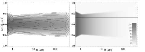
Figure 7: Density structure of the model disc. Left: density distribution of the best fitting stationary model of the SED of May 31, 1997. The density contours are plotted as a function of the radial distance and the polar angle. The puffed-up inner rim ($r\leq 1.5$ AU) is opaque below a polar angle of $\sim$15^∘, puting most of the disc into the shadow. The line-of-sight is at about 20^∘. Right: Change of density in the disc between the two extreme models with surface density exponents -0.9 and -0.4. The solid line marks the line-of-sight.

Our model fits the continuum radiation over 3 orders of magnitudes in wavelengths, from the optical to the far-infrared, reasonably well. This result verifies that the assumed self-shadowed geometry is a very good description of the circumstellar environment. Local differences, however, appear in the 10–20 $\mu$m range where the model cannot reproduce the observed silicate emission features. The reason is that in the model the surface layer of the disc immediately behind the rim, where the silicate emission arises, is not illuminated. In reality, this region of the disc might be irradiated indirectly by stellar photons scattered in the rim photosphere, producing the observed emission features. An other possible explanation for the silicate emission features could be an optically thin halo around the star + disc system (see below). Also, our disc model is not able to fit the observed 1.3 mm flux. The age of SV Cep (4 Myrs) suggests that significant fraction of big grains ($r\sim 1\,mm$) may be settled in the disc midplane, which radiate at this wavelengths. Since these particles are in the disc midplane and have more or less grey opacities, their radiation should not vary.

Modelling light variations. After finding a stationary model which fits the SED of SV Cep at a reference epoch, one may try to model the observed flux variations. A possible origin of the flux variations can be that the illumination source of the circumstellar disc, e.i. the star itself, changes. However theoretical models predict the presence of an instability strip on the Hertzsprung-Russel Diagram (HRD) Boehm et al. (2004), the possible periods are in the order of an hour or even less. This periods are too short comparing with the observed timescale ($\sim$years) in the light curves of SV Cep. Thus our working hypothesis is that the optical variations are caused by long-term eclipses in the inner rim, produced by some effects in the rim which change its height along a significant fraction of its perimeter (rather than along the line of sight only). The eclipse nature of the phenomenon is supported by observations of Rostopchina et al. Rostopchina (2000), who showed that SV Cep turns redder when becoming fainter. This hypothesis predicts some consequences in the infrared regime. A higher inner rim, while obscuring the star, absorbs more stellar radiation which is re-emitted then as 2–8$\mu$m thermal emission. At the same time a higher rim results in stronger shadowing of the outer regions. Since the disc around SV Cep is thought to be passive, a stronger shadow results in a decreased radiation from the outer parts of the disc in the far-infrared domain. Because both the inner rim and the optically thin outer part of the disc are expected to react on the changes of the stellar illumination almost instantaneously, both the optical vs. mid-IR anti-correlation and the optical vs. far-IR correlation should be observable.

The prediction that the optical and far-infrared emission changes in the same direction is fully consistent with our observational results which exhibit correlation between the optical and far-infrared fluxes (Fig. 5). The predicted optical vs. mid-infrared anti-correlation seems also be consistent with the data, though in this case the observational results are less conclusive.

We tried to model our changing rim scenario quantitatively with the RADICAL and the RADMC. Since these codes are time-independent, stationary codes, our concept was to model the variability through a sequence of quasi-stationary states. In this process the variable height of the rim was simulated by changing the amount of matter in the rim area (i.e. the surface density at the inner edge of the disc). Here we assumed circular symmetry, i.e. the density of the rim was increased or decreased along its complete perimeter simultaneously. The vertical Gaussian density profile of the disc has a pressure scale height which is determined by the temperature and independent of the density Dullemond et al. (2001). Thus a higher surface density with the same pressure scale height causes higher volume density and higher opacity in the rim, and the photosphere of the rim moves up in vertical direction. In the course of modelling the variation of surface density at the inner edge of the disc was realized by changing the exponent of the power law of the surface density between -0.9 and -0.4. Figure 7 (right panel) shows the change of density in the whole disc between the two extreme models with exponents -0.9 and -0.4. The plot demonstrates that a modification of the exponent does not alter the structure of the outer disc considerably (the surface density was constant within 10%), but could efficiently be used for fine-tuning the surface density in the rim.

By gradually changing the exponent of the surface density (we emphasize that it was the only parameter tuned) we created a sequence of spectral energy distributions, from which we produced synthetic light curves and correlation diagrams. The results revealed that the amplitude of the infrared variations does not depend on the viewing angle, but the amplitude of the optical changes does. In order to match the relative amplitude of the optical and far-IR variations we played with the inclination angle; the best fitting value was $i=71^{\circ}$. The dashed lines in Fig. 5 mark linear fits to the synthetic correlation diagrams. The plots demonstrate that our numerical simulation of the changing rim scenario is able to reproduce the observed trends of the light variation in the optical, near- and far-infrared domains simultaneously.

Figure 8: SED of SV Cep. The measured data points are corrected for an interstellar reddening of 0.57^m. Overplotted is the best fitted disc$+$envelope model.

However, the model is not able to explain the mid-infrared behaviour of SV Cep. The predicted flux variations at 12 and 25 $\mu$m would have similar amplitude and direction (i.e. correlation with the optical) than was seen at 100 $\mu$m, in contrary to the observed almost constant brightness at these wavelengths. It is interesting to note that this is the same wavelength range in which the model SED was not able to fit the observed emission features.

It is a question whether the hypothetic changes in the amount of matter in the inner rim are physically reasonable? The rim contains less than 1% of the total disc mass. In our simulations we had to vary the rim mass between $10^{-4}-10^{-5}M_{\odot}$ on a time-scale of a few years. If this change was explained by varying accretion, the accretion rate would be in the range of $10^{-5}M_{\odot}$/yr; an unexpectedly high value for an old UX Orionis star. An alternative explanation would be to assume that the pressure scale height of the rim may also change due to some dynamic instabilities which affect a significant portion of the rim at the same time. Further analyses are needed to clarify the possible nature of the variations of the rim structure.

4.2.2 Disc$+$envelope model

Figure 9: Correlation diagrams between the optical and infrared light variations. All light curves are normalized for the reference day of May 31, 1997. Dotted lines are linear fits to the observations; dashed lines show the same for synthetic light curves obtained from modelling using a disc$+$envelope system (Sect. 4).

Since the pure disc model is not able explain the observed behaviour of SV Cep at mid-infrared wavelengths (12–25 $\mu$m) we tried to find an alternative solution. The lack of variability suggests that the heating source of the matter emitting at these wavelengths is independent of the height of the inner rim. An obvious way to meet this criterion is the introduction of an optically thin envelope around the system. Since the envelope is a spherical structure it can be illuminated by the central star continuously, the inner rim has no significant effect on the irradiation of the envelope. Moreover an optically thin envelope could produce the observed huge silicate emission features around 10 and 20 $\mu$m.

Modelling the SED. On purely physical grounds we are able to constrain some property of the envelope. If the inner radius would be smaller than 10 AU, the variability would disappear around 3.6 $\mu$m, due to the contribution of the envelope emission to the SED. On the other hand, if the inner radius would be greater than 30–40 AU, the dust temperature would not be high enough to produce the emission feature at 10 $\mu$m. Thus we set the inner radius to 15 AU, while the outer radius of the envelope was set to 500 AU which was also the outer radius of the grid.

There are disc$+$envelope models in the literature which explain the 2–8 $\mu$m emission in Herbig Ae/Be stars by invoking a compact ($\sim$10 AU), tenuous (${\tau}_{V}{<}{\sim}0.4$) dusty halo around the disc inner regions, rather than by assuming an inner rim (Vinkovic et al. 2006). Since the observations showed variability at the 2–8 $\mu$m region, which cannot be explained in the case of an envelope, we do not adopt the model of Vinkovic et al. Vinkovic (2006).

Dust grains of two different sizes (0.01 and 0.1 $\mu$m) were used to produce the emission features around 10 and 20 $\mu$m. The volume density distribution used in the model ($\rho(r)\propto r^{-2}$) was typical of an infalling envelope. The only fitted parameter of the envelope was the volume density at the outer radius of the envelope; its best fit value was $\rho_{0}=3.0\times 10^{-20}$ g/cm³. The applied disc parameters were the same than in the case of the pure disc model except for a few. The best fit disc model had a mass of $10^{-3}$ M_⊙ and the grain sizes were somewhat larger (0.75 and 3 $\mu$m) than in the envelope. The lower disc mass results in a geometrically thinner disc, thus the inclination angle in the best fit model was modified to 76^∘ in order to obtain the same optical variability than in the pure disc model.

The resulting fit to the spectral energy distribution is displayed in Fig. 8. It can be seen that the fit of this model to the continuum part of the SED is as good as in the case of the pure disc model. In the mid-infrared domain around 10 $\mu$m the fit of the disc$+$envelope model is remarkably better than that of the pure disc model.

Modelling light variations. The disc$+$envelope model can successfully reproduce the observed SED, but we also have to investigate the predicted light variations of this model at different wavelengths. The optical variability was simulated in the same way as in the case of the pure disc model (i.e. varying of the height of the inner rim). During this simulation the power index of the surface density distribution was tuned between -0.9 and -0.4. Then correlation diagrams were constructed from the synthetic light curves of different wavelengths. Figure 9 shows that the disc$+$envelope model is able to reproduce quantitatively the observed flux variations both in the optical and the 2–8 $\mu$m region and the anti-correlation between them. The model predictions in the mid-infrared domain around the silicate features are much closer to the observations than in the case of the pure disc model. Since the envelope radiates most of its energy around 10 and 20 $\mu$m and its emission is practically constant, the lack of flux variations at these wavelengths is not surprising. However in the far-infrared domain this model seems to be in clear conflict with the observations: it predicts an almost completely constant flux in contrary to the observed prominent variability at these wavelengths.

The reason of the lack of variability at far-infrared wavelengths is probably the heating of the outer parts of the disc by the envelope. In a disc$+$envelope model the outer regions of the circumstellar disc have two heating sources: radiation from the central star and from the envelope. The shadowing effect of the inner rim in this model is so strong, that the outer parts of the disc absorb more energy from the envelope than from the central star. Further than 10 AU from the star this process results in higher temperatures in the disc compared to a pure disc model. Since the flux emitted by the envelope is constant in time, the far-infrared flux will also be constant.

4.3 Comparison of the models

A systematic comparison of fitting the observed phenomena in the pure disc and the disc$+$envelope models is presented in Tab. 3. It can be seen that neither of the models is able to explain all the phenomena together. As was mentioned in Sec. 6 the quality of the fits could probably be improved by taking into account the scattering of stellar light which provides extra heating to the disc region where the silicate emission features originate. Modelling the far-infrared variability is, however, still a critical issue. In the disc$+$envelope model the temperature distribution of the outer parts of a self-shadowed disc is determined by the absorbed energy from the envelope. As discussed before, radiation of the envelope is not expected to show temporal variation, thus it is hard to find a way to produce far-infrared variability in such a model. Since far-infrared variability was definitely detected in our dataset, this is a strong argument against the disc$+$envelope model. The pure disc model might be a better starting point to model successfully the structure and behaviour of the circumstellar environment of SV Cep.

Observed phenomenon	Pure disc	Disc$+$envelope
SED continuum	Yes	Yes
SED emission features	No	Yes
Optical variability	Yes	Yes
NIR variability	Yes	Yes
MIR variability	No	Yes
FIR variability	Yes	No

Table 3: Summary of the relations between the observed phenomena and the predictions of the two different models.

5 Summary and Outlook

We investigated the long-term optical-infrared variability of SV Cep, and tried to explain it in the context of the self-shadowed disc model proposed for UX Orionis stars. A 25-month monitoring programme, performed with the Infrared Space Observatory in the 3.3–100 $\mu$m wavelength range, was carefully analysed, and the infrared light curves were correlated with the behaviour of SV Cep in the V-band. A remarkable correlation was found between the optical and the far-infrared light curves. In the $2-8\,\mu$m regime the amplitude of variability is lower, with a hint for a weak anti-correlation with the optical changes. No observable flux changes were recorded around 25 $\mu$m.

In order to interpret the observations, we modelled the spectral energy distribution of SV Cep assuming a self-shadowed disc with a puffed-up inner rim, using a 2D radiative transfer code. The simulations revealed that the main body of the SV Cep disc is located in the shadow of the inner rim (confirming the expected self-shadowed geometry), but a moderate flaring is also present in the outer disc which makes it possible that some cold tenuous regions far above the disc midplane can be directly illuminated by the star. We found that by modifying the height of the inner rim, the wavelength-dependence of the long-term optical-infrared variations is well reproduced, except the mid-infrared domain. The origin of variation of the rim height might be temporal changes in the accretion rate, but other mechanisms which alter the pressure scale height of the rim might be necessary to invoke. In order to model the mid-infrared behaviour we tested adding an optically thin envelope to the system, but this model failed to explain the far-infrared variability.

We demonstrated that infrared variability is a powerful tool to discriminate between existing models. The proposed mechanism of variable rim height may not be restricted to UX Orionis stars, but might be a general characteristic of intermediate-mass young stars. However, in star with pole-on view no optical changes are expected. Further infrared variability studies among Herbig Ae/Be stars would be needed to confirm this prediction.

References

- (1) Ábrahám, P., Kun, M. 2004, Baltic Astr. 13, 464
- Bertout (2000) Bertout, C. 2000, A&A, 363, 984
- (3) Bessel, M.S. 1979, PASP, 91, 589
- (4) Chiang, E.I., Goldreich, P. 1997, ApJ 490, 368
- Boehm et al. (2004) Boehm, T., Catala, C., Balona, L., Carter, B. 2004, A&A, 427, 907
- Dullemond et al. (2001) Dullemond, C.P, Dominik, C., Natta, A. 2001, ApJ, 560, 957
- (7) Dullemond, C.P., van den Ancker, M.E., Acke, B., van Boekel, R. 2003, ApJ, 594, L47
- (8) Dullemond, C.P., Hollenbach, D., Kamp, I., D’Alessio, P. 2006, in Reipurth, B., Jewitt, D., Keil, K., eds, Proc. Protostars and Planets V (in press)
- Gabriel et al. (1997) Gabriel, C., Acosta-Pulido, J., Heinrichsen, I., Morris, H., Tai, W.-M. 1997, PASPC, 125, 108
- Grady et al. (2000) Grady, C.A., Sitko, M.L., Russell, R.W., Lynch, D.K., Hanner, M.S., Perez, M.R., Bjorkman, K.S., de Winter, D. 2000, in Protostars and Planets IV. ed. Mannings, V., Boss, A. Russel, S. (Tucson: Univ. Arizona Press), 613
- Kun et al. (2000) Kun, M., Vinkó, J., Szabados, L. 2000, MNRAS, 319, 777
- (12) Laureijs, R.J., Klaas, U., Richards, P.J., Schulz, B., Ábrahám, P. 2003, The ISO Handbook, vol. V, ESA SAI-99-069/Dc, Version 1.2
- Lemke et al. (1996) Lemke D., Klaas U., Abolins J. et al. 1996, A&A 315, L64
- Meeus et al. (2001) Meeus, G., Waters, L.B.F.M., Bouwman, J., van den Ancker, M.E., Waelkens, C., Malfait, K. 2001, A&A 365, 476
- Natta et al. (1997) Natta, A., Grinin, V.P., Mannings, V., Ungerechts, H. 1997, ApJ, 491, 885
- (16) Rostopchina, A.N., Grinin, V.P., Shakhovskoi, D.N., Thé, P.S., Minikulov, N.Kh. 2000, Astronomy Reports, 44, 365
- (17) Vinkovic, D., Ivezic, Z., Jurkic, T., Elitzur, M. 2006, ApJ, 636, 348