A method to remove residual OH emission from near infrared spectra

Abstract

I present a technique to remove the residual OH airglow emission from near infrared spectra. Historically, the need to subtract out the strong and variable OH airglow emission lines from 1–2.5 micron spectra has imposed severe restrictions on observational strategy. For integral field spectroscopy, where the field of view is limited, the standard technique is to observe blank sky frames at regular intervals. However, even this does not usually provide sufficient compensation if individual exposure times are longer than 2–3 minutes due to (1) changes in the absolute flux of the OH lines, (2) variations in flux among the individual OH lines, and (3) effects of instrumental flexure which can lead to ‘P-Cygni’ type residuals. The data processing method presented here takes all of these effects into account and serendipitously also improves background subtraction between the OH lines. It allows one, in principle, to use sky frames taken hours or days previously so that observations can be performed in a quasi-stare mode. As a result, the observing efficiency (i.e. fraction of time spent on a source) at the telescope can be dramatically increased.

1 Introduction

Near infrared airglow emission originates in OH radicals which are created by reactions between ozone and hydrogen high in the atmosphere. Removing the emission lines which result from the subsequent radiative cascade is a crucial part of processing near infrared (1–2.5µm) spectra. While they are usually considered to be a nuisance in this respect, they also provide a useful reference for wavelength calibration (Oliva & Origlia, 1992; Maihara et al., 1993; Osterbrock et al., 1996; Rousselot et al., 2000).

Maihara et al. (1993) has measured the strongest lines, which lie in the H-band, to have fluxes of order 400 ph s^-1 m^-2 arcsec^-2. This contrasts strongly with the background continuum they measured between the lines of only 590 ph s^-1 m^-2 arcsec^-2 µm^-1. These values demonstrate that, even at a moderate spectral resolution of $R\sim 3000$, the background level on an OH line can be more than 3 orders of magnitude higher than that between them. There are inevitably implications both for the statistical photon noise and also for systematic effects when attempting to remove the OH emission by subtracting a ‘sky’ spectrum from an ‘object’ spectrum. The first of these noise sources is unavoidable, and can only be improved by integrating longer. The latter is an issue because the OH line fluxes can vary significantly on timescales of only a few minutes; and yet for a clean subtraction, the flux of the OH lines in the sky and object frames would have to differ by much less than 1%.

The flux variations are generally not a problem for longslit spectra, because the slit is usually much more extended than the object of interest: 120″ in the case of ISAAC (Moorwood et al., 1998) at the VLT. With such data, the OH emission can be completely removed from the rectified 2-dimensional spectrum: at each spectral pixel, one can fit a function to the residual background along the spatial dimension and subtract it.

Near infrared integral field spectrometers do not allow this because of the restricted field of view: there is no point in the observed field of view more than a few arcsec from the centre. For example, the largest field of view of SINFONI (Eisenhauer et al., 2003a, b; Bonnet et al., 2004) at the VLT is $8\arcsec\times 8\arcsec$; and at the finest pixel scale used with adaptive optics it is less than 1″. Similarly, OSIRIS (Larkin et al., 2006; Krabbe et al., 2006) for use with adaptive optics at the Keck II telescope has a field of view ranging from $0.32\arcsec\times 1.28\arcsec$ to a maximum of $4.8\arcsec\times 6.4\arcsec$ depending on pixel scale and spectral coverage. And the GNIRS IFU (Allington-Smith et al., 2006) for Gemini South telescope has a field of view of $3.15\arcsec\times 4.46\arcsec$. The KMOS (Sharples et al., 2005) multiple integral field unit which is being designed for the VLT will have individual fields of $2.8\arcsec\times 2.8\arcsec$. It is clear that in general astronomical targets will fill a substantial fraction – and perhaps all – of the field in any of these IFUs. As a result, one cannot easily extrapolate the background level from pixels at the edge of the field of view to those in the centre. For example, in crowded stellar fields such as the Galactic Centre, the combination of nebular emission, dust continuum, and faint stars make it challenging to identify any region of pure background in the central few arcsec. If one observes (active) galactic nuclei, although the emission may be dominated by a bright compact nucleus, there is still easily detectable extended emission out to more than a few arcsec. And in high redshift galaxies which one may expect to be only $\sim 1$″ across, there may be line emission on larger scales – for example Förster Schreiber et al. (2006) were able to detect line emission across 2–3″ in several $z>2$ galaxies. Thus in most cases it is mandatory to observe separate blank sky fields.

Compounding the problem is the demand to reach the maximum signal-to-noise even between the OH lines which requires exposure times of individual frames be 5–10 mins, to avoid their being read-noise limited. Hence, even if one takes frequent sky frames, the OH lines are almost always imperfectly subtracted.

The situation is complicated further by the fact that in such instruments the spectral line profile can vary across the field of view due to image distortions, off-axis aberrations, and manufacturing variations between elements. Thus one cannot simply take a sky spectrum from one spatial pixel and subtract it from another. This is also the reason why attempts to generate model OH spectra that can be subtracted from the data inevitably fail. To make matters worse, at moderate resolution the strength of the OH lines means that even small amounts of spectral flexure in an instrument (corresponding to only a few percent of a resolution element) can leave a significant ‘P-Cygni’ shape residual when a sky frame is subtracted.

The rather complicated topic of background subtraction for integral field spectrometers has been addressed by Allington-Smith & Content (1999). To reduce the effects of temporal uncertainty in the background, they proposed osberving a simultaneous blank sky field. This paper explores an alternative technique for removing the variable OH airglow without the need for a simultaneous sky frame.

2 Compensating for variable OH line fluxes

Figure 1: Top: Spectrum of a sky subtracted 5 min SINFONI exposure showing residual OH lines after subtracting a sky frame taken immediately afterwards. The flux in these residuals is only $\sim 3$% of the original OH emission, but is still significant. Bottom: the same two frames are subtracted using the scaling procedure described in the text in Section 2. The spectra are of NGC 3783 and in both cases were extracted within a 0.5″ aperture centered slightly off the galaxy nucleus. The reduction in noise is discussed quantitatively in Section 4 and shown in Fig. 7.

In this section a method which allows one to compensate for variations in both absolute and relative flux of the OH lines between object and sky frames is presented. These variations give rise to residuals such as those in Fig. 1 which, although only a few percent the original line strength, are still very significant.

The basis of the technique is to find a scaling as a function of wavelength that can be applied to a spectrum extracted from a sky cube in order to match it optimally to the sky background in an object cube. The scaling function is then applied separately to the spectrum at each spatial position of the sky cube individually, creating a modified sky cube. It is the entire modified sky cube that is then subtracted from the object cube – conveniently avoiding the issue of the variable spectral line profiles.

The scaling function can be found relatively easily if one understands the origin of the variation in the OH line fluxes. The relative populations of the excited states in the OH radical can be approximated well by Boltzmann distributions characterised by rotational and vibrational temperatures (e.g. Rousselot 1997). A rotational temperature of 205$\pm$5 K was found by Williams (1996) in Antarctica, which corresponds well to models of the kinetic temperature at the 85 km altitude where OH radicals exist. Although the vibrational temperature would have to be unphysically high, in the range 8500–13000 K (Wallace, 1968), it does provide a good representation of the intensities in the different bands.

2.1 Vibrational Variations

Figure 2: Spectrum of the OH emission across the H- and K-bands (the thermal background has been subtracted). The various spectral ranges corresponding to the different vibrational transitions (labelled) are indicated. Very few OH lines from the $7-5$ transition are observed due to atmospheric absorption (between the H- and K-bands) at these wavelengths.

It is between the vibrational bands that most of the variation in the OH spectrum occurs. Fortuitously, transitions between any two particular vibrational bands tend to lie, to a large extent, within well defined wavelength limits. These are shown for the H-and K-bands in Fig. 2. Furthermore, there is only some small overlap between different vibrational transitions; and within the overlap, the OH lines originating from either one or the other vibrational transition tend to be relatively weak. Thus, to a first approximation one can divide the spectrum into sections corresponding to specific vibrational transitions, and treat these separately.

It is this that the algorithm outlined below has been developed to do. A flow chart which includes these steps is given in Fig. 3.

1. identify the spatial pixels in the object cube which contain the least flux (typically 50% of the spatial pixels are selected).

2. sum spectra from these positions in both the object and sky cubes to create an object spectrum and a sky spectrum.

3. Fit a blackbody function to the thermal background in the sky spectrum, and subtract it from the sky spectrum as well as the original sky cube (to leave just the line emission).

4. for each spectral segment (corresponding to each vibrational transition) do the following:

   1. extract a vector array containing the few spectral pixels around each of the major OH lines in the sky segment and concatenate them into a single array (equivalently one can select all pixels which have a flux above some fraction, such as 20%, of the maximum in that segment).

   2. Repeat the extraction and concatenation for the object segment using the same pixels, but also subtracting the continuum for each OH line (it can be interpolated from spectral regions immediately either side of each line).

   3. find the scaling factor which minimizes the difference between the sky and object vectors.

   4. if there are any pixels in the object vector which deviate significantly from zero when the scaled sky vector is subtracted, reject them and repeat steps (a)–(c) above. This makes the procedure robust against any line emission from the science target that coincides with an OH line.

5. combine the scalings from each segment to generate the vibrational scaling function across the whole spectrum.

6. multiply the spectrum at each spatial position in the sky cube (from which the thermal background has been subtracted) by the scaling function to create a modified sky cube.

7. subtract the modified sky cube from the object cube.

The procedure as given above is not specific to OH lines, and hence can also be used for the jungle of emission features longward of 2.35µm in the K-band as well as the O₂ emission in the J-band.

An additional advantage comes from the fact that the scaling for each segment is derived from the stronger emission lines but is applied to the whole segment. This means that the weak unresolved OH continuum is also scaled similarly, providing a better quality background subtraction even between the obvious emission lines.

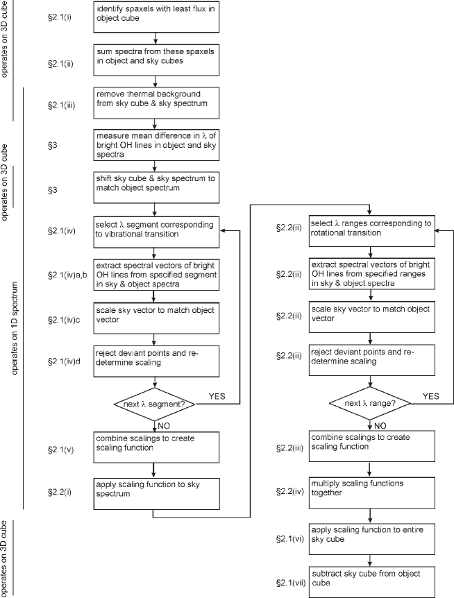
Figure 3: Flowchart showing the steps in the combined algorithm to correct both for changes in the vibrational and rotational temperature of the OH radical, and also for spectral flexure. Next to each step is indicated the place from where it comes in the text. Also shown is whether each step applies to a summed 1-dimensional spectrum or to the entire data cube.

2.2 Rotational Variations

Figure 4: Spectrum of a 5 min SINFONI exposure which has had the sky subtracted using the algorithm described in Section 2 to account for changes in the vibrational temperature. The residual shown is typical of what is seen with a change in the rotational temperature: the lines from the lowest upper level – Q1(1.5) and P1(2.5) – are over- (or equivalently under-) subtracted.

Refining the procedure to take into account changes in the rotational temperature of the OH radicals can quickly become rather more complex at the spectral resolutions of $R\sim 3000$ considered here. The reason is that there are many emission lines from different rotational levels whose wavelengths coincide and are blended at this resolution. Nevertheless, there are still a few distinct groups of lines which can be scaled together. Fig. 4 shows a residual – after correcting the sky subtraction for changes in the vibrational temperature as already described in Section 2.1 – typical of a change in the rotational temperature. The lines from the lowest upper rotational level of the $X^{2}\Pi_{3/2}$ sub-state, the P1(2.5) and Q1(1.5) transitions from the $J_{up}=3/2$ level (see Fig. 2 of Rousselot et al. 2000), are over-subtracted. This means that this group of lines can be corrected together – hence preserving robustness against line emission from the object occuring at the same wavelength as an OH line – using a single additional scaling which can be computed in a way analagous to that described previously.

If this is done, one then sees a new set of lines over-subtracted: the P1(3.5), Q1(2.5), and R1(1.5) rotational transitions from the $J_{up}=5/2$ level. This is where the difficulties begin, because for each vibrational transition the Q1(2.5) lines are only 10–20Å from the Q1(1.5) lines. At a spectral resolution of $R\sim 3000$ these are only a few resolution elements apart and hence still blended in their wings. Thus one cannot cleanly isolate them in order to apply an appropriate correction. Nevertheless, one can still make a significant improvement by simply excluding the Q1(2.5) lines from this group and correcting the others.

Thus a straight-forward implementation can be made using three groups of rotational transitions: the P1(2.5) and Q1(1.5) lines; the P1(3.5) and R1(1.5) lines; and the rest of the spectrum (the scaling for this being determined from all the remaining isolated lines). This leads to three scalings which can be multiplied into their respective parts of the vibrational scaling function to yield the final scaling function. The algorithm, which is included in the flow chart shown in Fig. 3, is then as follows:

1. having created a vibrational scaling function, multiply this into the sky spectrum.

2. for each set of wavelength ranges corresponding to the rotational transitions given above, perform exactly the same steps as described in (iv) a–d of Section  2.1.

3. combine the scalings from each set of wavelength ranges to generate the rotational scaling function across the whole spectrum.

4. multiply the vibrational and rotational scaling functions together.

5. continue at step (vi) of Section  2.1, multiplying the whole sky cube by the combined scaling function

While this does not provide a full correction for changes in the rotational temperature, it can – particularly in the H-band – make a significant enhancement on correcting only for the vibrational temperature.

It is worth noting that a simpler alternative becomes possible if one has simultaneous observations of a blank sky region (see also Allington-Smith & Content 1999), as is possible with multi-object spectrometers. One could then target each line – or blend of lines – independently, irrespective of its transition, using a similar scheme to that described above: derive the respective scalings from the simultaneous sky observation (in a different slitlet or IFU) and apply them to the sky frame taken previously (in the same slitlet or IFU as the object frame).

3 Compensating for Instrumental Flexure

Figure 5: Top: Spectrum of a sky subtracted 5 min SINFONI exposure showing P-Cygni OH residuals, characteristic of spectral flexure between the object and sky frames. Bottom: the same two frames are subtracted using the flexure compensation procedure described in the text in Section 3. The spectra are of NGC 3783 and in both cases were extracted within a 0.5″ aperture centered slightly off the galaxy nucleus. The reduction in noise is discussed quantitatively in Section 4 and shown in Fig. 7.

Figure 6: Top: concatenated vector of spectral segments containing strong OH lines which are used to determine the spectral shift between the object and sky frames. The shift between sky and object frames for each OH line in this array corresponds to one data point in the bottom panel. Bottom: Measured offset as a function of wavelength, each point corresponding to one OH line in the vector above. This method allows one to measure the mean offset with an accuracy of at least 0.01 pixel; and also to detect any trend with wavelength that there may be.

Very often, particularly in instruments mounted at a Cassegrain focus or those at a Nasmyth focus which need to rotate, there can be flexure resulting in shifts of the wavelength scale between exposures. Here we are concerned only with spectral shifts (regardless of the actual cause), since even small shifts can have a dramatic impact on the quality of the OH line subtraction. For example, subtracting 2 lines with the same flux but shifted by only 0.1 times the FWHM can leave a P-Cygni shape residual with an amplitude of more than 10% of the original line. A case where this has occured in SINFONI data is shown in Fig. 5. Once such residuals are created – for example by subtracting a sky frame from an object frame without correcting the shift a priori – they are extremely difficult to correct.

The obvious remedy is to apply a shift to the sky frame before subtracting it from the object frame. However, raw frames are not appropriate for this operation for 2 reasons: firstly, there will be numerous bad pixels which would normally be subtracted out but instead will propagate during the necessary interpolation; secondly, it is difficult to measure the required shift from raw spectra which contain significant curvature. Instead, a sequence of alternative data processing steps is outlined below:

1. subtract dark frames from both object and sky frames (rather than subtracting sky frames from the object frames directly) so that the OH emission remains in every frame.

2. reconstruct the object and sky cubes from the dark subtracted frames.

3. create a ‘thermal background’ cube from each sky cube (e.g. by running the routine described in Section 2 but using each sky frame as both the ‘object’ and ‘sky’ input).

4. subtract the appropriate thermal background cubes from each object cube (if the thermal background cubes do not change much, it may be possible to average them all to improve the signal-to-noise).

5. remove the OH emission from each object cube by using the routine described in Section 2, but also applying a shift to the wavelength scale of the respective sky cube as described below.

A method which has proven successful for measuring spectral shifts is to determine the position of every strong OH line in both the sky and object spectra – either by calculating the line centroids or by fitting Gaussian functions. This then yields a series of offsets as a function of wavelength, as shown in Fig. 6. It is usually sufficient to take the iterative mean of these, rejecting outliers which deviate significantly, and apply it as a constant shift to the entire sky spectrum. As indicated in Fig. 3, a couple of steps to measure and apply this shift can easily be included immediately after step (iii) of the routine described in Section 2.1. The same shift would also have to be applied to the complete modified sky cube before subtracting it in step (vii) of the same routine.

4 Towards Efficient Observing: a Quasi-stare mode

Figure 7: Noise in blank sky subtracted H-band SINFONI cubes (arbitrary data units) for consecutive 5 min integrations. The noise is measured across the whole field of view and in the wavelength range 1.55-1.75µm. Pluses denote cubes which each had a different sky cube, taken immediately afterwards, subtracted. Diamonds are the same, except the sky subtraction was performed using the routines described in this paper. Asterisks denote cubes from which the same sky cube (taken at the time indicated by ‘S’) was subtracted, also using these routines. The increase in noise for frames observed more than 30 mins after S is due to variations in the rotational temperature of the OH lines, which is only partially compensated.

Figure 8: Noise in blank sky subtracted K-band SINFONI cubes (arbitrary data units) for consecutive 10 min integrations taken on 2 nights. The noise is measured across the whole field of view and in the wavelength range 2.00–2.25µm (where the OH emission is most prominent). Pluses denote cubes which each had a different sky cube, taken immediately afterwards, subtracted. Diamonds are the same, except the sky subtraction was performed using the routines described in this paper. Asterisks denote cubes from which the same sky cube (taken at the time indicated by ‘S’) was subtracted, also using these routines.

In this section the performance of the strategies above are illustrated quantitatively using a sequence of 24 H-band SINFONI frames, each a 5 min exposure, taken during October 2005. These are nodded observations of a $z=1.4$ galaxy which is spatially compact (occupying less than 1″ of the 8″ field width) and has a rather faint continuum so that in a single exposure it is barely detected. Thus, for the purpose here, these frames in effect form a series of consecutive blank sky frames. Fig 7 shows the noise in the reconstructed cubes. The sky was subtracted in 3 ways. In one instance, for each frame the subsequent one was used as the ‘sky’ and simply subtracted, yielding 23 independent cubes. The mean noise in these was 9.91 ADU, but there is a great deal of variation depending on whether the OH lines happen to subtract well or not. For the second instance, the routines described in Sections 2 and 3 were used to optimise the subtraction. The mean noise in each of these cubes was much less, being only 5.86 ADU, and much more stable; when the first 9 were combined, the noise in the resulting cube was 1.99 ADU, close to that expected. In the third instance, only a single sky frame (close to the middle of the sequence, denoted by ‘S’ at time zero) was subtracted from every other cube using the routines described previously. In all cases, the noise is less than that reached by simply subtracting the nearest sky frame, and for a period of about 30 mins before and after the sky frame was taken, the noise in the resulting cubes was comparable to that of the cubes processed optimally with their own sky frames. Combining 9 of these frames (with small 2 pixel spatial dithers between them) yielded a cube with a noise of 2.07 ADU.

From these results one can conclude that even when using sky frames taken after each object exposure, the background subtraction can be improved – often significantly – by using the algorithms described here. Furthermore, they enable one to achieve comparable or better background subtraction even when using a sky frame taken at a different time. Thus, a similar noise level can been reached but in a much shorter amount of observing time: in the example above, one needs only a single sky frame rather than 9. Hence the observing efficiency can be increased from 50% to 90% without loss of signal-to-noise.

The increase in noise for the frames which were observed more than 30 mins before or after the sky frame is due to variations in the rotational temperature of the OH lines – which is only partially compensated in the scheme described in this paper. In the H-band, where the OH lines are strongest, this appears to be a limiting factor. On the other hand, a similar test with K-band data have shown that in most cases one can use sky cubes taken on different nights without losing signal-to-noise. Fig. 8 shows the results of the test involving 21 exposures of 10 min taken over 2 nights. Again, these are nodded observations of a high redshift galaxy at $z=2.4$ which is compact (also filling less than 1″ of the 8″ field width) and is only detected even in line emission after multiple integrations – thus an individual exposure is effectively blank. The noise in each of the resulting cubes has been measured in the wavelength range 2.00–2.25µm, where the OH emission is most prominent and the thermal background is relatively low. Individual frames which each had their own separate sky cube simply subtracted had a mean noise of 16.11 ADU across both nights, but with considerable variation as was found in the H-band test. When the sky subtraction was optimised, the mean noise was reduced to 11.57 ADU and the stability significantly improved. When 7 of these optimised cubes are combined, the noise in the resulting cube was 4.56 ADU, close to the expected value. Cubes from which a single sky cube taken on the same night was subtracted had a mean noise of 12.14 ADU; even when the sky cube was observed on a different night, the mean noise in the processed cubes was still the same at 12.06 ADU. In all cases an optimal sky subtraction using the single frame was better than a simple subtraction using a frame taken immediately afterwards. When 7 such cubes from each night are combined (using 2 pixel spatial dithers), the resulting noise is 6.09 ADU and 6.07 ADU. Thus by using only a single sky frame one loses slightly in terms of signal-to-noise but gains significantly in terms of telescope time: each of the latter combined cubes required only 80 mins of open shutter time, whereas the former combined cube required 140 mins.

Based on the tests above, it seems reasonable to conclude that it is not necessary to observe a sky frame immediately before or after each object frame – i.e. that one does not need to spend 50% of the time observing blank sky, as has historically been done. Sky subtraction works equally well using a frame taken 30–60 mins before (and for K-band the frames can in principle be taken days apart). A strategy in which a sky frame is taken only once per hour rather than every other exposure would represent a significant step towards observing in a ‘stare’ mode. As long as there are small (e.g. 2 pixel) dithers between the pointings of each object frame, the noise in the sky frame will not add coherently when all the sky-subtracted cubes are combined. This is valid as long as one wishes to preserve the spatial information (e.g. to generate line maps or velocity fields) rather than sum the spectra over a large aperture. For near infrared integral field units where the small field of view means little or no region of blank sky is included, this could improve the observing efficiency by nearly a factor of 2.

5 Conclusions

I have presented a method by which the OH emission in the near infrared bands can be removed. The technique takes into account variations in the absolute and relative OH lines as well as instrumental flexure, which may impact the wavelength scale. It has been tested using observations performed with the integral field spectrometer SINFONI.

When the field of view is too small to include blank sky, I have shown that rather than taking separate blank sky frames at every other exposure, one can adopt a much more efficient observing strategy. In principle, one needs to take a sky frame only once per hour in the H-band where the OH lines are particularly strong; and less often for K-band observations. This allows the fraction of time spent on source to be increased from 50% to as much as 90% or more.

A version of the code used to perform these procedures is written in IDL and is available from the author. In addition, the routines are being implemented in the SINFONI data processing pipeline by ESO. The essence of the procedure has also been incorporated into the data processing software specification (Davies & Förster Schreiber, 2006) of KMOS, a near infrared multi-IFU spectrometer for the VLT (Sharples et al., 2005).

References

- Allington-Smith & Content (1999) Allington-Smith J., Content R., 1999, PASP, 110, 1216
- Allington-Smith et al. (2006) Allington-Smith J., Content R., Dubbeldam C., Robertson D., Preuss W., 2006 MNRAS, 371, 380
- Bonnet et al. (2004) Bonnet H., et al., 2004, The ESO Messenger, 117, 17
- Davies & Förster Schreiber (2006) Davies R., Förster Schreiber N., 2006, ESO/KMOS preliminary design review document VLT-SPE-KMO-146611-001
- Eisenhauer et al. (2003a) Eisenhauer F., et al., 2003a, The ESO Messenger, 113, 17
- Eisenhauer et al. (2003b) Eisenhauer F., et al., 2003b, in Instrument Design and Performance for Optical/Infrared Ground-based Telescopes, eds. Masanori I., Moorwood A., Proc. SPIE, 4841, 1548
- Förster Schreiber et al. (2006) Förster Schreiber N., et al., 2006, ApJ, 645, 1062
- Krabbe et al. (2006) Krabbe A., Larkin J., Iserlohe C., Baraczys M., Quirrenbach A., McElwain M., Weiss J., Wright S., 2006, in Ground-based and Airborne Instrumentation for Astronomy, eds. McLean I., Masanori I., Proc. SPIE, 6296, 151
- Larkin et al. (2006) Larkin J., et al., 2006, in Ground-based and Airborne Instrumentation for Astronomy, eds. McLean I., Masanori I., Proc. SPIE, 6296, 42
- Maihara et al. (1993) Maihara T., Iwamuro F., Yamashita T., Hall D., Cowie L., Tokunaga A., Pickles A., 1993, PASP, 105, 940
- Moorwood et al. (1998) Moorwood A., et al., 1998, The ESO Messenger, 94, 7
- Oliva & Origlia (1992) Oliva E., Origlia L., 1992, A&A, 254, 466
- Osterbrock et al. (1996) Osterbrock D., Fulbright J., Martel A., Keane M., Trager S., Basri G., 1996, PASP, 108, 277
- Rousselot (1997) Rousselot P., 1997, “Calculation of the OH infrared spectrum (preliminary report)”
- Rousselot et al. (2000) Rousselot P., Lidman C., Cuby J.-G., Moreels G., Monnet G., 2000, A&A, 354, 1134
- Sharples et al. (2005) Sharples R., et al., 2005, The ESO Messenger, 122, 2
- Wallace (1968) Wallace L, 1968, “OH bands in the airglow”, Kitt Peak National Observatory, Contribution N142
- Williams (1996) Williams P., 1996, P&SS, 44, 163