Modeling GRB 050904:
Autopsy of a Massive Stellar Explosion at $z=6.29$

Abstract

GRB 050904 at redshift $z=6.29$, discovered and observed by Swift and with spectroscopic redshift from the Subaru telescope, is the first gamma-ray burst to be identified from beyond the epoch of reionization. Since the progenitors of long gamma-ray bursts have been identified as massive stars, this event offers a unique opportunity to investigate star formation environments at this epoch. Apart from its record redshift, the burst is remarkable in two respects: first, it exhibits fast-evolving X-ray and optical flares that peak simultaneously at $t\approx 470$ s in the observer frame, and may thus originate in the same emission region; and second, its afterglow exhibits an accelerated decay in the near-infrared (NIR) from $t\approx 10^{4}$ s to $t\approx 3\times 10^{4}$ s after the burst, coincident with repeated and energetic X-ray flaring activity. We make a complete analysis of available X-ray, NIR, and radio observations, utilizing afterglow models that incorporate a range of physical effects not previously considered for this or any other GRB afterglow, and quantifying our model uncertainties in detail via Markov Chain Monte Carlo analysis. In the process, we explore the possibility that the early optical and X-ray flare is due to synchrotron and inverse Compton emission from the reverse shock regions of the outflow. We suggest that the period of accelerated decay in the NIR may be due to suppression of synchrotron radiation by inverse Compton interaction of X-ray flare photons with electrons in the forward shock; a subsequent interval of slow decay would then be due to a progressive decline in this suppression. The range of acceptable models demonstrates that the kinetic energy and circumburst density of GRB 050904 are well above the typical values found for low-redshift GRBs.

1 INTRODUCTION

One of the most exciting results from the first year of operations of NASA’s Swift satellite mission (Gehrels et al. 2004) has been the discovery and observation of GRB 050904 (Cusumano et al. 2006) at redshift $z=6.29$ (Kawai et al. 2006). This burst was initially detected by the Swift BAT at 01:51:44 UT on September 4, 2005, and was quickly followed up by pointed observations with the X-ray telescope (XRT) and UV/optical telescope on Swift, and by numerous ground-based facilities. Early afterglow photometry provided the first indications for a very high redshift for this event, $z>5.3$ (Haislip et al. 2005), prompting a global observing campaign that culminated in the spectroscopic observations by Subaru that provided the redshift (Kawai et al. 2006) and enabled the first investigation of the reionization epoch via GRB afterglow light (Totani et al. 2006).

Within a day of the burst, the discovery of an associated prompt $I\approx 14$ mag optical/NIR flash was reported (Boër et al. 2006). The timing of this flare, which peaks at $t\approx 470$ s after the burst, is coincident with X-ray (XRT) and $\gamma$-ray (BAT) flares observed by Swift (Cusumano et al. 2007). This is the second such bright optical flash observed so far, after GRB 990123 (Akerlof et al. 1999), and may even exceed that event in optical luminosity (Kann et al. 2007).

Subsequent optical and NIR observations of the fading afterglow were reported by Haislip et al. (2006) and Tagliaferri et al. (2005), and provide evidence for a slow decay phase during the first day after the burst, and a jet break at $t\approx 3$ days. A campaign of radio observations at the VLA yielded multiple detections of the afterglow at 8 GHz, which exhibited a slow evolution consistent with a high circumburst density and extremely high kinetic energy (Frail et al. 2006). The X-ray lightcurve observed by Swift exhibits numerous interesting features, including the early flare at $t\approx 470$ s, vigorous X-ray flaring activity, and a possible jet break (Cusumano et al. 2007). Finally, observations with the Hubble Space Telescope and the Spitzer Space Telescope by Berger et al. (2006) have yielded late-time detections of the afterglow and host galaxy.

Studies of GRBs at low-redshift, $1\lower 4.0pt\hbox{$\buildrel<\over{\sim}$}z\lower 4.0pt\hbox{$\buildrel<\over{\sim}$}3$ (Panaitescu & Kumar 2001a; Yost et al. 2003), have established that the circumburst densities for these events range between $0.06$ and $30\ {\rm cm^{-3}}$, with their kinetic energies having a relatively narrow distribution with a peak around $5\times 10^{50}\ {\rm ergs}$ (Panaitescu & Kumar 2002; Berger et al. 2003). It is therefore interesting to investigate whether the quantities for the high-redshift GRBs follow these results or not.

Several questions seem particularly pertinent. What density range is found in the environments of GRBs at high redshift? How do their kinetic energies compare to those of low-redshift events? Are other properties of high-redshift GRBs – their beaming angles and shock microphysical parameters – the same as for low-redshift GRBs? The answers to these questions can potentially cast light on outstanding mysteries of the GRBs themselves, and reveal important aspects of the early Universe. These interesting questions provide the motivation for our detailed investigation of the properties of GRB 050904.

In this paper, we attempt a complete model of the full set of X-ray, optical/NIR, and radio afterglow observations of GRB 050904. Our derivation of physical parameters from afterglow observations is carried out in the context of the fireball model (Mészáros 2006, and references therein).

We make explicit consideration of two scenarios for the origin of the X-ray and optical flares at $t\approx 470$ s. Our first scenario (A) attributes the flares to internal shocks or engine activity, and excludes the flares from afterglow fits, with only later observations considered. This is consistent with the approach of Wei et al. (2006), who argued on the basis of the fast decay of the flares that they could not be due to reverse shock emission. In our alternate scenario (B), however, we attribute the flares to emission from the reverse shock. In order to accommodate their fast decay, we use a starting time for the asymptotic Blandford-McKee solution which is near the start of the flare, later than the burst trigger time, which serves to flatten the post-flare decay. In this scenario, the optical flare comes from synchrotron radiation in the reverse shock, and the X-ray and $\gamma$-ray flares are produced by synchrotron self-Compton scattering (SSC) of photons in the reverse shock region. A cosmology where $H_{0}=71~{}{\rm km~{}s^{-1}~{}Mpc^{-1}},\Omega_{\Lambda}=0.73,~{}{\rm and}~{}\Omega_{m}=0.27$ is assumed in calculating the luminosity distance $D_{L}$. For GRB 050904 at $z=6.29$, the luminosity distance is $D_{L}=1.93\times 10^{29}$ cm.

Our model and its supporting analytical formulae are presented in §2, with several derivations reserved for the appendices. Our numerical simulation procedure and the data set used in our fits are described in §3, while in §4 we analyze the results, including the $J$-band light curve (§4.1), the radio light curve (§4.2), and our ultimate energy and density constraints (§4.3). A discussion of the results and our conclusions are presented in §5 and §6, respectively.

2 OBSERVATIONS AND THEORETICAL FRAMEWORK

2.1 Burst and Afterglow Observations

The Swift BAT observations of the prompt emission give a $\gamma$-ray duration of $T_{90}=225\pm 10$ s, a spectrum with power-law photon index $\Gamma=1.34\pm 0.06$, and a fluence of $\sim 5.4\times 10^{-6}\ {\rm erg\ cm^{-2}}$ (Cusumano et al. 2006). Given the burst redshift of $z=6.29\pm 0.01$, the isotropic-equivalent gamma-ray energy is $E_{\gamma,{\rm iso}}\sim 10^{54}\ {\rm ergs}$. XRT observations began 161 s after the burst and continued for 10 days after the burst trigger, overlapping with BAT observations for about 300 s before the high energy emission faded below the BAT threshold (Cusumano et al. 2006).

Thanks to the Swift prompt alert, the early afterglow was also observed promptly by the TAROT robotic telescope. The TAROT observations started at 86 s after trigger and lasted for more than 1500 s; by making a spectrophotometric calibration of the field, Boer et al. (2006) are able to present their data as flux densities at 9500 Å, which we use and shall refer to as the TAROT $I$-band observations. Other larger ground-based telescopes started imaging the field 3 hours later (Haislip et al. 2006; Tagliaferri et al. 2005). We present our compilation of the observational data in the X-ray (XRT), hard X-ray (BAT), and optical/NIR in Fig. 1. Here and throughout the paper we convert X-ray measurements to flux density measurements at the frequencies of 5 keV (XRT) or 50 keV (BAT); these energies correspond to observing frequencies of $1.2\times 10^{18}$ Hz (XRT) and $1.2\times 10^{19}$ Hz (BAT), respectively. The conversion factors from photon counts per second (cps) to flux are 3.31 $\mu{\rm Jy~{}cps^{-1}}$ for XRT PC data, 1.82 $\mu{\rm Jy~{}cps^{-1}}$ for XRT WT data, 154.6 $\mu{\rm Jy~{}cps^{-1}}$ and 86.2 $\mu{\rm Jy~{}cps^{-1}}$ for BAT masktag-lc data, respectively (see Cusumano et al. 2007 for the details of XRT PC, WT and BAT data).

As seen in Fig. 1, the flux and spectral evolution of the burst and afterglow divide the lightcurve into six distinct segments, determined by inspection and motivated by the physical model put forth herein. These segments are: (A) $t<350$ seconds: In the X-ray band, the flux decays as $F_{\nu}\propto t^{-\alpha}$ with an index of $\alpha=2.07\pm 0.03$ (Cusumano et al. 2006). We follow the conventional definition for the flux $F_{\nu}\propto t^{-\alpha}\nu^{-\beta}$. In the $I$-band observation, there are two observational data points, the earlier of which is only an upper limit, apparently indicating an increasing tendency of the flux with time. (B) $320<t<600$ seconds: Flares are observed in both the $I$ and X-ray bands, and also in the BAT energy range. They peak around 470 seconds after the burst trigger time. The spectral index evolves from $0.50\pm 0.07$ to $0.88\pm 0.12$ over this time interval. (C) $600<t<6.3\times 10^{3}$ seconds: A power-law decay is shown in the X-ray band. During the same time interval, there is no optical/NIR detection, except for two upper limit flux values at 9500 ${\rm\AA}$. (D) $6.3\times 10^{3}<t<4.3\times 10^{4}$ seconds: Many irregular fluctuations are observed in the X-ray band. The J band shows a decay which can be described with $\alpha=1.36^{+0.07}_{-0.06}$ (Haislip et al. 2006). (E) 0.5 days $(\approx 4.3\times 10^{4}\ {\rm seconds})<t<2.6$ days: There is no effective XRT observation within this period, and no further fluctuations are detected. The flux in the J band is flattened a little bit with a temporal index of $\alpha=0.82^{+0.21}_{-0.08}$ (Haislip et al. 2006) or $\alpha=0.72^{+0.15}_{-0.20}$ (Tagliaferri et al. 2005). (F) $t>2.6$ days: the flux decay index in J band is around $\alpha=2.4\pm 0.4$. Only one data point in the X-ray band is available. The J-band data shows a sharp break, which is thought to be the jet break.

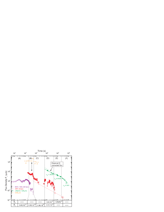
Figure 1: The combined light curves of GRB 050904 in the BAT, XRT, $J$ and $I$ bands, in the observer frame. The BAT (violet, empty triangle) and XRT (red, empty circle) data are taken from Cusumano et al. (2006), the early time $I$-band flare at 9500 $\rm\AA$ (orange, star) is from Boër et al. (2006), and the $J$-band data (green, solid circles) are from Haislip et al. (2006) and Tagliaferri et al. (2005). For ease of presentation, we show the BAT flux density divided by a factor 100. The black arrows at $t=398$ seconds after the burst indicate the adopted reference time point, in our model (B), for the start of the afterglow evolution. The solid line (green) shows the observed afterglow evolution in $J$-band. The dashed lines show the theoretically-expected afterglow evolution in the X-ray and $J$-band, respectively, and the dash line (green) is the light curve behavior in the J band without the external IC process by the X-ray photons from the flare. The light curve is divided into 6 sections labeled from A to F sequentially: (A) $t<225$ s: prompt emission; (B)$225<t<600$ s: simultaneous flares in the X-ray and NIR bands; (C) $600<t<6220$ s: power-law decay in the X-ray band; (D) $6220<t<4.3\times 10^{4}$ s: energetic X-ray flaring activity; (E) $0.5{\rm days}<t<1.6{\rm days}$: flattening of the light curve in the NIR band; (F) $t>1.6$ days: a jet break is apparent. Approximate temporal power-law indices ($F_{\nu}\sim t^{-\alpha}$) in the optical ($\alpha_{o}$) are noted. Estimated spectral indices ($F_{\nu}\sim\nu^{-\beta}$) in the optical/NIR (observed and uncorrected for extinction) and X-ray are also provided, where available, in the lower figure panels below the figure. References for the spectral indices are (a) Haislip et al. (2006); (b) Tagliaferri et al. (2005); (c)-(f) Cusumano et al. (2006). A jet break time of $t_{\rm jet}=2.6\pm 1.0$ days has been reported by Tagliaferri et al. (2005); however our fit of all available data suggests instead $t_{\rm jet}=3.17\pm 0.22$ days.

2.2 Afterglow Modeling in the Swift Era

Thanks to the rapid and precise alerts generated by Swift, and its extensive multiwavelength follow-up campaigns, the afterglow data collected during the Swift era has resulted in some necessary modifications to the standard afterglow model.

Data from Swift have provided the greatest advance over earlier datasets in the X-ray band, as Swift responds to the burst orders of magnitudes faster than previous generations of satellites and can often track the X-ray afterglow for up to 10 days. Many new features of the X-ray afterglow have thus emerged, leading to the identification of a canonical X-ray afterglow behavior. In addition to the prompt emission phase, this involves at least five components of the X-ray afterglow (Nousek et al. 2006; Zhang et al. 2006a), which are: (1) A steep decay phase, often interpreted as the tail of the prompt emission, and thus, part of the GRB internal shock; (2) A shallow decay phase of uncertain origin, with several theoretical models proposed, including energy injection, jet inhomogeneities, or varying shock microphysical parameters; (3) A normal decay phase, familiar from pre-Swift observations; (4) A post jet break phase; and (5) The X-ray flares, which are superposed on the various power-law segments of the afterglow’s decay, and are fast-evolving in the sense that the flare’s rise and decay timescales $\delta t$ are much smaller than the time since the burst $t$, that is, $\delta t/t\ll 1$. The current interpretation ascribes the X-ray flares to the same cause as the prompt gamma-ray emission – energy dissipation in internal shocks (Zhang et al. 2006). Since the X-ray flares are thus a manifestation of central engine activity, it is necessary to exclude them from afterglow model fits (e.g., Falcone et al. 2006; Chincarini et al. 2007; Nava et al. 2007).

The accumulation of Swift afterglow observations has also raised questions about the collimated or “jet” interpretation of afterglow lightcurves. Traditionally, jets have been invoked to explain a late time ($t\lower 4.0pt\hbox{$\buildrel>\over{\sim}$}1.0$ day), broadband and achromatic steepening in the afterglow decay by an increment of +1 in the power-law index, from $\alpha\approx 1.2$ to $\alpha\approx 2.2$. Specifically, the late-time decay index is predicted on robust grounds to be $\alpha=p$, where $p$ is the power-law index of the energy distribution of the synchrotron-emitting electrons that generate the afterglow light.

Current challenges to the jet break picture are two-fold. First, there are few jet breaks seen in the X-ray light curves of afterglows observed by Swift (Burrows & Racusin 2007). As of 7 October 2006, the XRT had observed 145 long GRBs and 16 short GRBs, with the X-ray afterglows of almost all long bursts followed for days to weeks with Swift, in campaigns that typically last until 10 days after the burst. Unexpectedly, among these bursts, only 4 long bursts and 2 short bursts show the jet break signature (See Table 1, Burrows & Racusin 2007). Second, where X-ray breaks of the appropriate steepness are seen, they are often observed to be chromatic, exhibiting a different evolution in UVOT (or ground-based optical) observations. Thus the jet break picture is being reevaluated, with new possibilities, such as energy injection or the evolution of microphysical shock parameters, under active consideration (Panaitescu 2005).

Despite these results, we believe that the jet break picture remains the better interpretation for most bursts, even in the Swift era. First, the energetics of GRBs are extremely difficult to reproduce from stellar-mass progenitors without beaming corrections of some sort. Second, the successes of the standard jet break picture in modeling bursts from before Swift are too numerous and significant to be discounted (e.g., Harrison et al. 1999; Panaitescu & Kumar 2001b; Yost et al. 2003). Third, several candidate jet breaks have been identified in the Swift era, and when these are seen, they exhibit the expected properties (e.g., Cenko et al. 2007; Dai et al. 2007; Burrows & Racusin 2007).

Finally, several arguments support the presence of a jet break in the evolution of the afterglow of interest to us here, GRB 050904. The break that is observed in the NIR lightcurve of the afterglow at $t=2.6\pm 1.0$ day (Tagliaferri et al. 2005) is achromatic, being seen in multiple NIR bands, and is followed by a steep post-break decay with power-law index $\alpha=2.4\pm 0.4$, consistent with the closure relation expected from the standard jet model (Tagliaferri et al. 2005). Separately, combining the Ghirlanda relation (Ghirlanda et al. 2004), and expression for the jet break time (Sari et al. 1999), a jet break is expected in the range between 0.64 and 3.0 days. The peak energy of GRB 050904 is $E^{src}_{peak}\geq 150(1+z)=1095$ keV and its isotropic-equivalent gamma-ray energy lies between $6.6\times 10^{53}$ and $3.2\times 10^{54}$ erg (Cusumano et al. 2006), so we take $E^{src}_{peak}\sim 1100$ keV and $E_{\gamma,iso,52}\sim$ 100. In addition, the circumburst density lies between $40<n<1000\ {\rm cm^{-3}}$ (Kawai et al. 2006). Setting $n\sim 100\ {\rm cm^{-3}}$ and the radiation efficiency in the prompt emission phase $\eta_{\gamma}=0.2$, one can obtain the jet break ranges of 0.64 and 3.0 days from Eqn. 3 of Sato et al. (2007), which is consistent with the observed break time.

2.3 Two Different Scenarios

2.3.1 (A) Forward Shock Fit Only

It has been argued by Wei et al. (2006) that the flares at $t\approx 470$ s are due to internal shocks, rather than a reverse shock, based on an apparent steep decay of the X-ray light curve right after the peak, with a temporal index of $\alpha_{1}\approx 8.8$ when referenced to the burst trigger time (see Kobayashi & Zhang 2007 for a discussion on the onset of GRB afterglow). This is because the fastest decay must not be steeper than that from the high latitude emission, whose temporal index is $\alpha_{2}=\beta+2$, in this case, $\alpha\approx 3$. This leads them to favor internal shocks for both the optical and X-ray flares, or a combination of reverse shock for the optical and internal shocks for the X-ray. Consistent with this argument, we investigate a model of the forward-shock emission only, that is, we consider only data points in regions (C)-(F) of Fig. 1.

2.3.2 (B) Forward Shock and Flares Fit

Separately, we consider a scenario in which the flares peaking at $t\approx 470$ seconds in the optical and X-ray are due to the reverse shock. This is motivated by the following argument. First, from the observational point of view, the flares of GRB 050904 have a great similarity with the behavior of GRB 990123, which is thought to be due to the reverse shock (e.g., Sari & Piran 1999). Second, the Blandford-McKee (BM) solution (Blandford & McKee 1976) describing the afterglow is parameterized with a time origin $t_{0}$ given by the trigger time. However, the BM solution is an asymptotic description of the afterglow evolution, which is valid for times substantially longer than any of the timescales associated with the prompt emission. Clearly, however, there is a transition from the initial prompt phase, when the bulk Lorentz factor is relatively constant, to the steady deceleration phase when the asymptotic BM solution applies. Numerical simulations have so far not provided specific guidance on the most appropriate value of the reference time for BM (afterglow) evolution.

Naturally, however, the steepness of the light curve decay, as parameterized by $F_{\nu}\sim(t-t_{0})^{-\alpha}$, depends on the reference time $t_{0}$ that is adopted. This has been discussed most recently in the context of the X-ray flares seen by Swift, which exhibit steep decays and so are widely attributed to internal shocks (Liang et al. 2006). Here we are dealing with a somewhat different situation, in that the X-ray light curve exhibits an initial flare and a subsequent decay, which we propose to attribute to a reverse shock. In the absence of guidance from numerical simulations, we adopt a purely phenomenological approach, based on the constraint that, whether for internal shocks or for a reverse external shock, the temporal decay cannot be steeper than $(t-t_{0}^{{}^{\prime}})^{-\alpha}$, where $t_{0}^{{}^{\prime}}$ is the reference time which fits the high latitude decay $\alpha=2+\beta$, where $\beta$ is the spectral index. For late central engine internal shocks, $t_{0}^{{}^{\prime}}$ is found to be near the onset of the last spike (Liang et al. 2006). Here, in the same spirit, since the initial X-ray flare is assumed to be due to the reverse shock, after which the BM solution is asymptotically reached, the new reference time $t_{0}^{{}^{\prime}}$ is determined from the constraint that the decay slope be equal to that expected from the high latitude mechanism. Having set a new reference time $t_{0}^{{}^{\prime}}$, all the time-related quantities for the afterglow evolution, such as $\nu_{m},\nu_{c}$ and so on, are now referred to $(t-t_{0}^{{}^{\prime}})$. We emphasize, however, that although the reference time is shifted from the burst trigger time to a new time point, the physical deceleration timescale remains the usual one. For GRB 050904, the best-fitting reference time satisfying the high latitude condition is $t_{0}^{{}^{\prime}}=(0.86\pm 0.01)t_{dec}$, where the (usual) deceleration timescale is 468 s (and the latter is measured relative to the burst trigger time).

The deceleration time is a critical point in the afterglow evolution. After that, both the reverse shock and the forward shock evolve into the asymptotic regime of the BM solution. In model (B), the peak time should represent the deceleration time of the shock. In the discussion below all the formulae after the deceleration time are taken relative to new reference time $t_{0}^{{}^{\prime}}$ (we have inserted the exact value of $t_{0}^{{}^{\prime}}$ into the equations below). A difference between models (A) and (B) lies in that $t_{0}^{{}^{\prime}}=0$ for model (A) and $t_{0}^{{}^{\prime}}>0$ for model (B). The determination of $t_{0}^{{}^{\prime}}$ for model (B) will be described in §3.1.

2.4 Synchrotron and Inverse Compton Afterglow Model

The flares in the optical (Boër et al. 2006) and X-ray (Cusumano et al. 2006) are observed to peak simultaneously at $t\approx 470$ seconds after the burst. The X-ray data has better time resolution, with an estimated peak time of $t_{\rm peak}=468.0\pm 2.0$ s.

We consider fits for two generic models, as described above. In model (A) the flares are ignored, as they may come from other regions (possibly internal shocks) rather than the reverse shock region. In model (B), however, we consider the flares to be due to the reverse shock. In this case, since the peak of the flare is clearly separated from the GRB itself, the reverse shock must be in the thin-shell regime (Zhang et al. 2003). Spectral analysis (Boër et al. 2006) shows that the flares in the X-ray and optical bands must be due to different mechanisms. Here, we assume that the optical flare is due to synchrotron radiation in reverse shock region, and that the X-ray flare is produced by synchrotron-self-Compton (SSC)in the reverse shock region (e.g., Wang et al. 2001; Kobayashi et al. 2007). Other observed X-ray components at late times, except for the flares, are assumed to be produced by synchrotron radiation from the forward shock. We use the following reference values for the main parameters involved: the isotropic-equivalent kinetic energy $E_{52}=1$, the external circumstellar density $n=1\ {\rm cm^{-3}}$, and the magnetic field ratio of the reverse and forward shocks $R_{B}^{2}\equiv\epsilon_{B,r}/\epsilon_{B,f}$. In addition, we have assumed equality of the energy equipartition parameter for electrons in the forward and reverse shock regions in model (B).

A transition from the temporal index $\alpha=0.82\pm 0.08$ to $\alpha=2.4\pm 0.4$, interpreted as the jet break, is observed at $t_{\rm jet}=2.6\pm 1.0$ days (Tagliaferri et al. 2005), and the sharpness of this break makes the burst not likely to have occurred in a stellar wind-type density environment (Kumar & Panaitescu 2000; Gou et al. 2001; Frail et al. 2006). Therefore, we will focus on afterglow evolution in a uniform density environment throughout the paper.

2.4.1 Forward Shock Synchrotron Formulae

Usually the synchrotron emission spectrum of the forward shock is described by a broken power-law with three critical quantities $\nu_{m}$, $\nu_{c}$, and $F_{\nu,{\rm max}}^{\rm syn}$ which are the synchrotron frequencies for the electron energies at the injection, cooling and peak flux emission, respectively (Sari et al. 1998). In modeling the radio emission, it is necessary to also take into account the self-absorption frequency, $\nu_{sa}$. We present the formulae including self-absorption in Appendix A, because there are different forms depending on various afterglow regimes, six in all, for the spectra given by Granot & Sari (2002). The main quantities of interest are:

$$\nu_{m,f} = 2.65\times 10^{23}\ {\rm Hz}\ \left(\frac{p-2}{p-1}\right)\epsilon_{B,f}^{1/2}\epsilon_{e}^{2}\left(t-t_{0}^{{}^{\prime}}\right)^{-3/2}\left(\frac{1+z}{7.29}\right)^{1/2}$$ (1)

$$\nu_{c,f} = 1.58\times 10^{15}\ {\rm Hz}\ E_{52}^{-2/3}\epsilon_{B,f}^{-3/2}n_{0}^{-1}\left(t-t_{0}^{{}^{\prime}}\right)^{-1/2}\left(1+Y\right)^{-2}\left(\frac{1+z}{7.29}\right)^{-1/2}$$

$$F_{\nu,max,f}^{syn} = 7.63\times 10^{-5}\ {\rm Jy}\ \epsilon_{B,f}^{1/2}E_{52}n_{0}^{1/2}\left(\frac{D_{L}(z)}{1.9\times 10^{29}}\right)^{-2}$$

where the convention $Q=10^{x}Q_{x}$ is used, kinetic energy $E=10^{52}E_{52}$ erg, and density $n=1\ n_{0}$ cm^-3. $\epsilon_{B}$ is the magnetic field equipartition parameter, and $\epsilon_{e}$ is the electron equipartition parameter. The subscript “$f$” denotes the forward shock, and “$r$” denotes the reverse shock. The parameter $Y$ refers to the first-order inverse Compton effect and is defined as $Y=(-1+\sqrt{1+\eta\epsilon_{e}/\epsilon_{B,f}})/2$ (Sari & Esin 2001). Here $\eta$, the fraction of the electron energy that is radiated away, expresses the magnitude of the radiative correction: $\eta=1$ for fast cooling and $\eta=(\gamma_{c}/\gamma_{m})^{2-p}$ for slow cooling, where $\gamma_{c}$ is the cooling Lorentz factor and $\gamma_{m}$ is the typical Lorentz factor for the electrons. For $z=6.3$, the luminosity distance in a concordance cosmology is $D_{L}\sim 1.9\times 10^{29}$ cm. After the deceleration time, relative to the new reference time, the afterglow will evolve asymptotically as the BM solution. Thus, the evolution relation for each quantity is $\nu_{c}\propto(t-t_{0}^{{}^{\prime}})^{-1/2},\nu_{m}\propto(t-t_{0}^{{}^{\prime}})^{-3/2}$, and $F_{\nu,m}\propto(t-t_{0,}^{{}^{\prime}})^{0}$.

The quoted typical values for $\nu_{m}$, $\nu_{c}$ and $F_{\nu,{\rm max},f}^{\rm syn}$ are consistent with the ones in Granot & Sari (2002), but the values for $\nu_{m}$ and $\nu_{c}$ are 2 times smaller, and the typical value for $F_{\nu,{\rm max},f}^{\rm syn}$ is 4 times smaller than that in Sari et al. (1998), which are fitted for the numerical simulation results.

2.4.2 Reverse Shock Synchrotron Formulae

In the reverse shock at the deceleration time, the typical quantities are (Kobayashi et al. 2007):

$$\nu_{m,r}=\nu_{m,f}R_{B}R_{M}^{-2},\ \nu_{c,r}=R_{B}^{-3}R_{X}^{2}\nu_{c,f},F_{\nu,max,r}=R_{B}R_{M}F_{\nu,max,f}$$ (2)

where $R_{B}\equiv(\epsilon_{B,r}/\epsilon_{B,f})^{1/2}$, $R_{X}\equiv(1+Y)/(1+X)$, $X=(-1+\sqrt{1+\eta\epsilon_{e}/\epsilon_{B,r}})/2$ is the Compton parameter in the reverse shock region, and the factor $R_{M}\equiv\Gamma_{d}^{2}/\Gamma_{0}$, where $\Gamma_{d}$ is the Lorentz factor at deceleration time. For the thin-shell case, $\Gamma_{d}\approx\Gamma_{0}$, so we have $\Gamma_{M}\approx\Gamma_{0}$ (Zhang et al. 2003).

After the deceleration time, since the shock is in the thin-shell case, each quantity evolves as $\nu_{c}\propto(t-t_{0}^{{}^{\prime}})^{\alpha_{c}}$ where $\alpha_{c}={(15g+24)/(14g+7)}$, $\nu_{m}\propto(t-t_{0}^{{}^{\prime}})^{\alpha_{m}}$ where $\alpha_{m}={-(15g+24)/(14g+7)}$, and $F_{\nu,m}\propto(t-t_{0}^{{}^{\prime}})^{\alpha_{f}}$ where $\alpha_{f}={-(11g+12)/[7(1+2g)]}$ (Zou et al. 2005) where $g$ is the evolution index for $\Gamma\propto R^{-g}$ where $\Gamma$ is the Lorentz factor of the afterglow, and $R$ is the radius of the afterglow.

2.4.3 Inverse Compton Effects, Jet Break and Non-relativistic Case

Both models include inverse Compton effects. The formulae for the normal case $\nu_{a}<\nu_{m}<\nu_{c}$ and $\nu_{a}<\nu_{m}<\nu_{c}$ in the forward shock case are listed in Sari & Esin (2001). We have derived the formulae for additional cases where the self-absorption frequency is above the typical frequency $\nu_{m}$ or cooling frequency $\nu_{c}$ in Appendix B. For inverse Compton effects in the reverse shock, the self-absorption frequency has a similar form as that of the forward shock, the only difference being that the forward shock-related quantities are replaced by the corresponding reverse-shock quantities.

Before the bulk Lorentz factor drops below the inverse of the opening half-angle, $\theta^{-1}$, each of the typical quantities follows the evolution given above (see sections 2.4.1 and 2.4.2). After $\Gamma<\theta^{-1}$, those typical quantities follow a different evolution given by Sari et al. (1999).

We also consider the non-relativistic (NR) evolution of the afterglow in its end-state. The time for the afterglow to enter into the NR stage is calculated by the condition that the Lorentz factor of the shell $\Gamma=2$. After the afterglow evolves into the NR stage, its dynamics are described by the self-similar Sedov-von Neumann-Taylor solution, for which Frail et al. (2000) have given a detailed description.

2.4.4 Host Galaxy Extinction and Lyman-$\alpha$ Damping Absorption

We have considered the host galaxy extinction in the optical band in the rest frame of the host galaxy, using a Milky Way extinction curve. We note that the particular type of extinction curve used is not expected to make a difference in this case; Kann et al. (2007) have tested the application of SMC, LMC, and Milky Way extinction curves to the composite J-band data, and all three models suggest minimal extinction. In our fitting, we treat the visual extinction $A_{V}$ in the host galaxy as a free parameter. In addition, because the extinction affects the spectral shape, we have considered the spectral index correction due to the host galaxy extinction in our fitting.

Besides the normal extinction by the host galaxy, the emission close to the wavelength of Lyman-$\alpha$ at $z=6.29$, including $z$ band emission (effective wavelength $0.91\ \mu m$ and band width is $0.13\ \mu m$), has undergone neutral hydrogen absorption in the IGM. Totani et al. (2006) fit the spectrum of GRB 050904 and find its best-fit column density to be $\log N_{HI}(\rm cm^{-2})=21.62$. To find the expected Lyman-$\alpha$ absorption in the $z$ band, we have convolved the Lyman-$\alpha$ absorption profile with the filter transmission curve of the $z$-band, and obtain the absorption coefficient $A=0.77$ meaning $33\%$ loss of $z$-band flux.

Also we notice that from Figure 6 in Totani et al. (2006), the absorption around wavelength $9500{\rm\AA}$ is negligible, so we take the absorption efficient $A=1$ for the 9500 Å data.

3 Fitting Data and Procedure

3.1 Observational Data and Constraints

Our model fits for the two different scenarios cover a range of bands from the radio, through the IR/optical, to X-ray and BAT energies. The list of the observational data used in our global fitting is in Table 1.

Table 1: Reverse and Forward Shock Observation Data Points

No.	Obs. Time	Obs. Freq.	Band	Flux(Error)
	log10(t[sec.])	log10($\nu$[Hz])		($\mu Jy$)
1	2.66	14.6	$I$	5.	1(10) $\times 10^{4}$
2	2.66	18.1	5 keV	70.	4 (44)
3	2.66	19.1	50 keV	4.	45 (89)
4	2.86	18.1	5 keV	0.	65(26)
5	3.25	18.1	–	0.	32(7)
6	4.75	18.1	–	0.	32(10) $\times 10^{-2}$
7	5.46	18.1	–	0.	51(17)$\times 10^{-3}$
8	2.78	14.6	$I$	12.	8(64) $\times 10^{3}$
9	4.98	14.4	$J$	19.	1(73)
10	5.27	14.4	–	9.	2(17)
11	5.56	14.4	–	2.	74(19)
12	5.66	14.4	–	1.	67(32)
13	5.79	14.4	–	0.	42(21)
14	4.98	14.27	$H$	23.	70 (21)
15	5.26	14.27	–	10.	60 (10)
16	6.30	14.27	–	8.	0(25) $\times 10^{-2}$
17	4.99	14.14	$K_{s}$	33.	70(210)
18	5.27	14.14	–	15.	0(10)
19	4.94	14.51	$z$	9.	12(19)
20	5.03	14.51	–	6.	92 (10)
21	4.97	14.46	$Y$	14.	0(30)
22	5.29	14.46	–	8.	4(22)
23	4.64	9.9	Radio	89.	0(580)
24	5.08	9.9	–	41.	0(250)
25	5.67	9.9	–	-3.	0(250)
26	5.73	9.9	–	27.	0(240)
27	6.24	9.9	–	89.	0(370)
28	6.40	9.9	–	40.	0(300)
29	6.46	9.9	–	-10.	0(350)
30	6.47	9.9	–	64.	0(230)
31	6.48	9.9	–	116.	0(180)
32	6.51	9.9	–	67.	0(170)
33	6.58	9.9	–	13.	0(270)

In model (A), the new reference time is the trigger time, so $t_{0}=0$. In model (B) with the flares included, we have to determine the new reference time first. We will now describe our procedure for the early time data used as input to the fits of model (B). Relative to the trigger time, the temporal index of the fast decay is $\alpha\approx 8.8$. The fast decay is considered to be due to the high latitude emission of the reverse shock. In order to obtain the new reference time, we assume a simple power-law model for the high latitude flux $f_{\nu}=F_{\nu}(\frac{t_{obs}-t_{0}}{t_{p}-t_{0}})^{-\alpha}$, where $F_{\nu}$ denotes the peak flux at the peak time $t_{p}$, $t_{0}^{{}^{\prime}}$ is the starting time at which the asymptotic Blandford & McKee solution applies, and $\alpha$ is the temporal index. The high latitude emission is assumed to decay with an index $\alpha_{h}=2+\beta$. For the X-ray observations right after the peak, $t>470$ seconds after the burst, the observational spectral index is around $\beta=0.88\pm 0.12$, so we take the temporal index in the fitting as $2.88\pm 0.12$, and selecting two observed data points, we can find the new reference time to be $(0.86\pm 0.01)t_{dec}$. In our fitting, we have set the new reference time at $0.86t_{dec}$.

We notice that right after the fast decay starting 470 seconds after the burst there is a plateau, extending from $t\approx 600$ seconds to $t\approx 2000$ seconds (see Fig. 2). A close look at the data around 1000 seconds shows an obvious flare, so we ignore the data after that. Thus, we only keep the X-ray data between 470 seconds and 1000 seconds. For this part of the data, there are three different contributions: (1) Forward shock; (2) High-latitude emission of the flare; (3) High-latitude emission of the prompt emission. It should be pointed that the high latitude emission of the prompt emission must be described by a broken power-law due to the spectral evolution of the burst itself (Cusumano et al. 2006); the break time in the rest frame is at $t\approx 350$ s in the observer frame. Before the break time, the temporal index is $\alpha\approx 2$, and afterwards, it is $\alpha\approx 3$. We subtract the high latitude emission from the observed flux to obtain the “pure” forward shock emission. To reduce the uncertainty of the data points, we then find the mean flux by averaging adjacent data points in groups of five, and use the averaged value for our fitting, finally providing the fourth data point in Table 1.

We also apply a similar subtraction method to the data around $t\sim 2000$ seconds indicated in Fig. 2. The averaged data point is the 5th row in Table 1. One difference between the subtraction for the fourth and fifth data points is that we only consider the flare contribution for the fifth data point (the prompt emission is considered negligible here), while both the flare and the high latitude emission of the prompt emission are considered for the fourth data point.

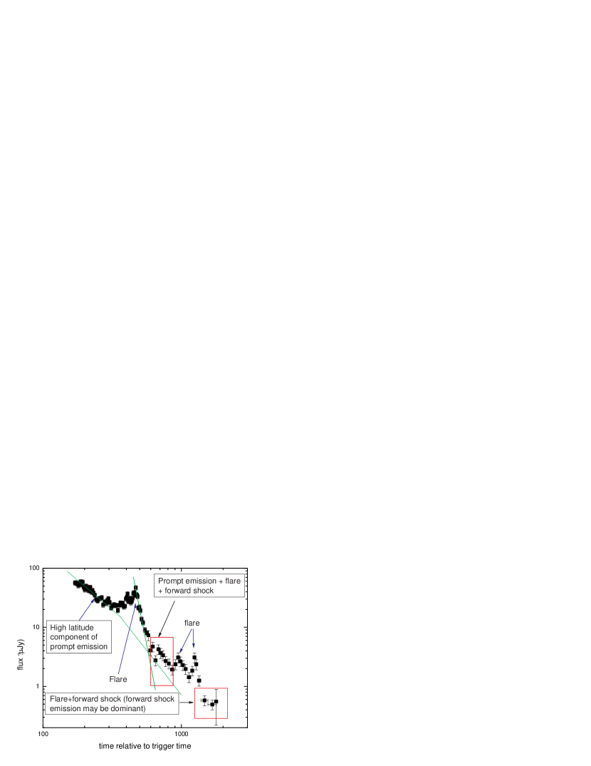
Figure 2: Illustration of the multiple mechanisms contributing to the observed flux at early times. The high-latitude component of the prompt emission is described by a broken power-law with a break time of $t\approx 350$ s in the observer frame (Cusumano et al. 2006). Before the break time, $\alpha\approx 2$ and afterwards, $\alpha\approx 3$. The main flare peaks at $t=468.0\pm 2.0$ s after the burst. The black data points correspond to the observed flux. The green lines indicate the theoretical extrapolation of the high-latitude emission to late times, using the best-fit values of the burst and flare emission without any subsequent fitting. The red-color boxes indicate the data used for estimating the forward shock emission.

Table 2: Other observational constraints for the fitting

Constraint	Comments	Reference
$t_{\rm jet}=3.17\pm 0.22^{\tablenotemark{1}}$	Jet break time	1
$t_{\rm dec}=468.0\pm 2.0^{\tablenotemark{2}}$	Deceleration time	2
$\beta_{J}=1.25\pm 0.25^{\tablenotemark{3}}$	Spectral index in $J$ band at t=1.155 days	3
$\beta_{\rm X}=0.96\pm 0.19^{\tablenotemark{4}}$	Spectral index in X-ray from t=680 and 1600 s.	4

The common constraints considered in both model (A) and model (B) are the following: (1) The jet break time is fitted to be $3.17\pm 0.22$ days (1-$\sigma$) by combining all available NIR and X-ray data. Kann et al. (2007) have extrapolated all the other NIR/optical data to the J band and made a composite light curve in the J band, including the HST data observed by Berger et al. (2006) $\sim 23$ days after the burst, and obtain a jet break time $t_{\rm jet}=2.63\pm 0.37$ days. Tagliaferri et al. (2005) give a value of $t_{\rm jet}=2.6\pm 1.0$ days based on multiband fitting of a smaller data set. (2) The spectral index in the $J$-band at 1.155 days is $1.25\pm 0.25$ (Tagliaferri et al. 2005). (3) The average spectral index for the early time X-ray afterglow from $t=680$ s to $t=1600$ s is $\beta=0.96\pm 0.19$ (Cusumano et al. 2006).

Besides the constraints above, we introduce another constraint for model (B): (4) the deceleration time is $t_{\rm dec}=468.0\pm 2.0$ s from our estimate of the peak of the X-ray light curve.

It should be mentioned that in model (B) we have summed over both the reverse and forward shock flux to fit the observed data ($I$, X-ray and BAT bands) at the deceleration time.

Thus, considering all the available data listed in Table 1, as well as the observed spectral index and the jet break time, we have 37 constraints for case (A) and 33 constraints for case (B).

For the fitting and (simultaneous) evaluation of parameter uncertainties, we perform a Markov Chain Monte Carlo analysis (MCMC; see Sec. 3.2 for a more detailed description). In order for the code to spend most of its time in the regions which have physical meaning, we provide penalty conditions during the calculation of the chi-square. The penalty is levied by giving an extra boost to the chi-square value when the penalty condition is violated (when the condition is satisfied, this extra chi-square is zero). To ensure the smoothness of the fit function at the penalty boundary, the penalty function we choose (more or less arbitrarily) is $\Delta\chi^{2}=[(x-x_{\rm lim})/(0.01*{\rm min(x,x_{\rm lim}}))]^{4}$, where $x_{\rm lim}$ is the critical value for each parameter.

We have included some upper limits in our dataset by converting the upper limits into synthetic measurements with error bars, as follows. Assuming all the upper limits as 2-$\sigma$ limits (we notice that the J band data labeled as No. 13 in Table 1 is provided as a 3-$\sigma$ upper limit, Tagliaferri et al. 2005; and the confidence level for the I band data, No. 8, is not stated, Boër et al. 2006), we take the measurement to be half the upper limit, and the error bar to be one-quarter the upper limit (half the synthetic measurement). For the radio data, which are provided as measurements with error bars even when no detection is realized, we adopt these measurements and error bars directly, while plotting 2-$\sigma$ upper limits in our figures.

For both models (A) and (B), the parameter ranges are restricted as follows: (1) $\epsilon_{e}\leq 0.5$; (2) $\epsilon_{B,r}\leq 0.5$; (3) $\epsilon_{B,f}\leq 0.5$; (4) Electron energy power-law index $p\geq 2.06$; (5) $\gamma_{m}>2.1$ at $t=10^{7}$ seconds after the burst. Violations of the parameter ranges incur chi-square penalties as discussed above, on a parameter by parameter basis.

Note that the critical electron energy index value (4) $p=2.06$ is found by equating the minimum electron Lorentz factor for the $p>2$ and $p=2$ cases. For $p>2$, the typical Lorentz factor $\gamma_{m}=\frac{(p-2)}{(p-1)}\frac{m_{p}}{m_{e}}\epsilon_{e}\Gamma$ (Sari et al. 1998). For $p=2$, $\gamma_{m}\approx\frac{1}{\ln{(4.0\times 10^{7})}}\frac{m_{p}}{m_{e}}\epsilon_{e}\Gamma$ .

Also note that, because we have assumed that the critical radiation mechanism is synchrotron radiation, the electrons in their shell frame are relativistic, and correspondingly $\gamma_{e}>2$ or $\gamma_{m}>2$ (because at late time the afterglow are in the slow-cooling regime, the Lorentz factor of the most electrons are concentrated at $\gamma_{m}$). We have set the critical value to be (5) $\gamma_{m}=2.1$ rather than $\gamma_{m}=2$ to eliminate the unrealistic parameter set corresponding to $\gamma_{m}\leq 2$.

We have not constrained the extinction parameter $A_{V}$, since in principle it can be any positive number; however, in order to avoid considering negative values of the extinction, the code makes use only of the absolute value of this quantity.

3.2 Parameters and Methodology

For model (A), we have 7 free parameters, which vary freely, subject only to the penalty conditions. The parameters are: the energy index $p$, the isotropic-equivalent kinetic energy in units of $10^{52}$ ergs $E_{52}$, the energy fraction in electrons in the reverse shock and forward shock regions $\epsilon_{e}$ (note that the electron equipartition parameter in the forward shock is assumed to be the same as the one in the reverse shock), the magnetic field equipartition parameter in the forward shock $\epsilon_{B,f}$, the circumburst density $n$, the jet opening half-angle $\theta$, and the extinction parameter in the host galaxy $A_{V}$. In model (B), we introduce two additional parameters: the magnetic field equipartition parameter in the reverse shock $\epsilon_{B,r}$, and the initial Lorentz factor $\Gamma_{0}$. We have assumed that the magnetic equipartition parameter in the forward and reverse shocks can be different, which is motivated by the results of Fan et al. (2002); Zhang et al. (2003); Kumar & Panaitescu (2003).

In order to obtain best-fit parameters and explore the parameter space of the fit function, we have tested both a grid search method and a Markov chain Monte Carlo (MCMC) method. However, we choose the MCMC after some tests. The grid-based likelihood analysis calculates chi-squared values at each grid point of the parameter space, and determines the best fit parameters and confidence levels by finding the minimum chi-square value point and range of values within a certain “height” above that minimum. The benefit of this method is primarily that it is straightforward. Once the parameter ranges and the number of grid points are defined, the code is easily implemented. However, the drawback is that it requires prohibitive amounts of time, especially if there are many free parameters. For example, a coarse grid with 7 points per dimension and with 8 parameters requires $2.1\times 10^{7}$ evaluations, and at 0.2 s per evaluation, the calculation takes $\tau\approx 5$ days on a single processor machine. Increasing the number of parameters, much less increasing the number of grid points, quickly becomes infeasible. By contrast, the MCMC method is very efficient, with execution time scaling linearly with the number of parameters, which allows us to perform likelihood analyses in a reasonable amount of time.

Briefly, the MCMC is a method to reproduce, directly, the posterior distribution of the model parameters (for a detailed treatment in an astronomical context, see Verde et al. 2003). After a limited “burn-in” phase, it should generate a random draw from the posterior distribution for most new function evaluations. From this sample, we can then estimate all of the quantities of interest for the posterior distributions (the mean, variance, and confidence levels). As mentioned above, the MCMC method scales approximately linearly with the number of parameters, allowing one to perform a likelihood analysis in a reasonable amount of time for a large number of parameters. After an initial burn-in period, and assuming that convergence of several chains can be established, all samples can be thought of as coming from a stationary distribution. In other words, the chain has no dependence on the starting location (although a good choice of starting points and step size can accelerate the chain convergence).

In implementing a MCMC approach, two key and interrelated questions are: (1) At what point does the chain converge, that is, how fast does the chain realize the target distribution?; and (2) Does the chain provide good mixing, that is, has the chain covered all interesting portions of the parameter space? Gelman & Rubin (1992) suggest a method to test the convergence and mixing and introduce for this purpose a parameter labeled $\hat{R}$ (see also Verde et al. 2003). The convergence can be monitored by calculating $\hat{R}$ for all the parameters in two or more chains, and running the simulations until all $\hat{R}$ values are less than 1.2. More conservatively, we may choose to run until all $\hat{R}<1.1$; this is the criterion we adopt as our test of convergence.

As we mentioned above, the MCMC model efficiently explores the parameter space, which guarantees that the global minimum will be approached in the long run. By contrast, in a grid search method, one has to provide the parameter range beforehand, and one is never sure that the minimum chi-square found is the global minimum instead of a local minimum. This can lead to very different results.

Before running the MCMC, it is necessary to initialize the starting point and assign step sizes for each parameter. For the starting point, we run a test chain first, then choose the best parameter set (evaluated by a minimum chi-square) as the starting point for a formal run. Initially, we set the step size for each parameter to be the 1-$\sigma$ range from this same initial run; however, several experiments convinced us that a half-sigma step size provided better convergence speed. Our MCMC code was implemented in a Matlab environment on a single processor machine, and then transplanted to the High Performance Computing (HPC) Linux cluster at Pennsylvania State University. We made use of 4 processors, each running one chain, and with each chain set to run for 2 million steps at a time. After the chain calculations are completed, we merge them and test for convergence. If the chains have not converged over the final 1 million steps of the 2 million-step chains, then we take the final parameter set as the starting point for another run, execute 2 million additional steps, and test for convergence again. The result for our final model, presented here, provided convergence after the first run in both cases (Models A and B), with $\hat{R}<1.1$ for all parameters after 2 million steps.

3.3 Numerical Results

For the results presented here, we ran four chains for $2\times 10^{6}$ steps for each of the models (A) and (B). Convergence was tested and parameters quantified using the final one million steps only. We found that both chains had already converged after the first run. For model (A) the $\hat{R}$ values are 1.008, 1.068, 1.045, 1.022, 1.076, 1.070, 1.004 for the parameters $p$, $\epsilon_{e}$ $\epsilon_{B,f}$ $n$, $\theta$, $E_{52}$, $A_{V}$, respectively. For model (B), the $\hat{R}$ values are 1.002, 1.004, 1.002, 1.004, 1.005, 1.005, 1.000, 1.004, 1.000 for the parameters $p$, $\epsilon_{e}$ $\epsilon_{B,f}$ $n$, $\Gamma_{0}$, $\theta$, $\epsilon_{B,r}$, $E_{52}$, $A_{V}$, respectively.

The posterior distributions for the parameters for model (A) are displayed in Fig. 3. The shaded blue regions delimit the 1-$\sigma$ range (68.2%-confidence), and the region included within vertical blue lines corresponds to the 90%-confidence interval. We choose the ranges of minimum width for these confidence intervals. Separately, we indicate the posterior distribution of model parameters for models with $\gamma_{m}<2.1$ (at $t=10^{7}$ s) in green, with a red color for its $1\sigma$ region. The number of model realizations that were constrained in this sense is roughly $1.5\%$ of the total trials. The reduced chi-square for model (A) reaches its minimum value $36.2/26\approx 1.39$, and the best fit parameters are $p=2.152$, $\epsilon_{e}=0.031$, $\epsilon_{B,f}=0.198$, $n=84.4$ cm^-3, $\theta=0.128$, $E_{52}=22.4$, and $A_{V}=0.034$ mag.

The light curve for the best fitting parameters is shown in Fig. 4 (indicated with solid line). We have shown the observational data as the background in the grey color, and indicated the data actually used for fitting in other bright colors (for detailed description on which color stands for which data, refer to the caption of the figure). We have plotted all of the data used, except for $Y$-band, $z$-band, and $K_{s}$-band data points, which may overlap with $J$-band data points if these non-J-band data are converted to $J$-band. For clarity of presentation, we convert non-$J$-band NIR data to $J$-band on the basis of the spectral index at that point, but still label it with its original band name and plot in a different color. At the bottom of the light curve figure, we show, as “residuals,” the chi-square contribution of each data point. We notice that the radio data provide a large contribution to the total chi-square, because of unexpected variations from observation to observation which are difficult to reproduce. In particular, the model fails to remain within the several upper limits from radio observations (note that eight out of 11 radio observations are upper limits, and three are flux measurements).

Fig. 4 also demonstrates the effects of the density on the afterglow evolution (shown in dashed and dotted lines, respectively). We notice that the X-ray and optical/NIR can be fitted well even for density values varying by 2 orders of magnitude; the only significant effects are seen in the radio light curve. The radio lightcurve for a density $n=10$ cm^-3 medium peaks around $t\sim 2.0\times 10^{6}$ s at a flux of $F_{\nu}\approx 200$ $\mu$Jy, that for a density $n=84.4$ cm^-3medium peaks around $t\sim 3.0\times 10^{6}$ s at $F_{\nu}\approx 100$ $\mu$Jy, and that for a density $n=10^{3}$ cm^-3 medium comes even later, at $t\sim 5.0\times 10^{6}$ s and $F_{\nu}\approx 120$ $\mu$Jy. At this point, the afterglow is in the regime with $\nu_{m}<\nu_{a}<\nu_{c}$, and the peak flux is at the self-absorption frequency. Because the self-absorption frequency is a function of density, the larger the density, the larger the self-absorption frequency. This predicts an earlier peak for a lower density. With more observational data points, or even upper limits after $t\sim 3\times 10^{6}$ s, we could put stronger constraints on the circumstellar density.

The posterior distributions for the parameters for model (B) are shown in Fig. 5. As for model (A), most of the distributions are satisfyingly Gaussian in shape. One exception is the magnetic field equipartition parameter $\epsilon_{B,r}$, seen to peak at $\epsilon_{B,r}=1/2$, the upper bound for $\epsilon_{B,r}$ in our model. Also, we note that the posterior distributions for the density $n$, the initial Lorentz factor $\Gamma_{0}$, and the opening half-angle $\theta$, have irregular tails. These irregular tail regions correspond to a distinct (local) chi-square minimum.

In the region where the reduced chi-square for model (B) reaches its minimum value $53.0/28\approx 1.9$, the best fit parameters are $p=2.243$, $\epsilon_{e}=0.0084$, $\epsilon_{B,f}=5.7\times 10^{-3}$, $n=212.4$ cm^-3, $\theta=0.126$, $E_{52}=146$, $A_{V}=0.032$ mag, $\Gamma_{0}=183.6$, and $\epsilon_{B,r}=0.50$. The light curve for these parameters is given in Fig. 6.

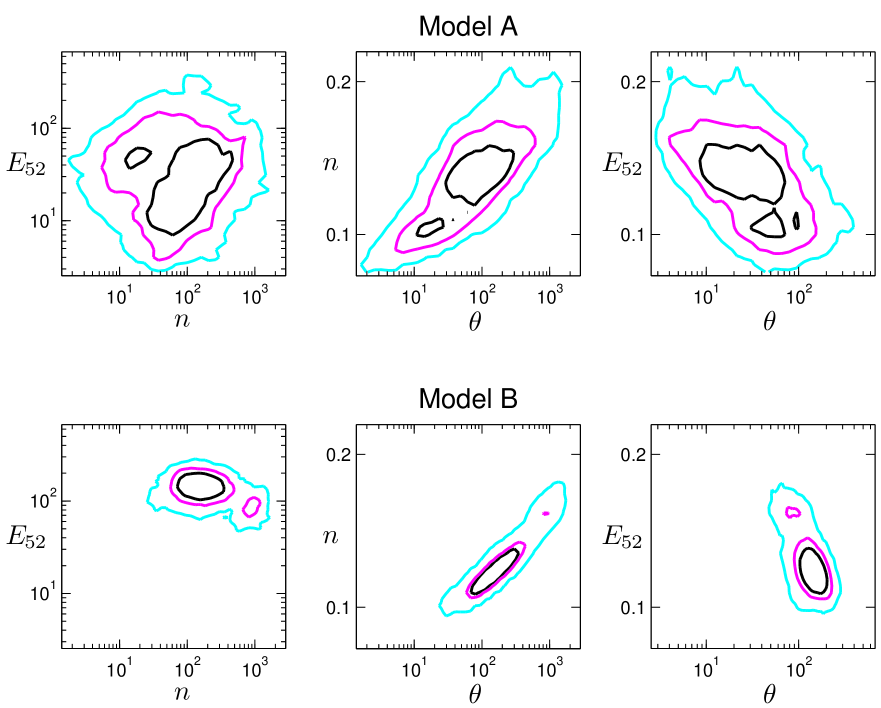
Figure 7: Joint confidence regions ($68\%,90\%,{\rm and}~{}99\%$, respectively) for three chosen parameters from our model fits: the jet opening half-angle $\theta$, the isotropic-equivalent kinetic energy $E_{52}$, and the circumburst density $n$. Top: Joint confidence regions for model (A), which excludes data related to the flaring activity at $t\approx 470$ s. Bottom: Joint confidence regions for model (B), in which the flares at $t\approx 470$ s are considered to be emission from the reverse shock regions. With the additional constraints available in model (B), the separate effects of blastwave kinetic energy and circumburst density can be distinguished, and the final constraints on the beaming of the burst and its total kinetic energy are significantly better-defined.

In Figure 7, we show contour plots for the joint confidence regions of three important physical parameters: the jet opening half-angle $\theta$, the isotropic-equivalent kinetic energy $E_{52}$, and the circumburst density $n$. This illustrates the degree of covariance between these quantities, in a quantitative manner.

In Table 3 we list the best-fitting parameters, and the parameter ranges for 1-$\sigma$ and $90\%$ confidence level for both models (A) and (B).

Table 3: The best fit values and parameter ranges for models (A) and (B).

	(A) Forward shock only			(B) Reverse shock flare
Parameters	Best Fit	1 $\sigma$ Range	$90\%$ Range	Best Fit	1 $\sigma$ Range	$90\%$ Range
$p$	2.15	2.11–2.19	2.09–2.22	2.24	2.20–2.29	2.18–2.32
$\epsilon_{e}(/10^{-2})$	3.09	4.3–14.6	2.8–26.3	0.84	0.75–1.3	0.66–1.6
$\epsilon_{B,f}(/10^{-2}$)	19.8	4.5–38.9	2.0–50.5	0.57	0.32–0.58	0.26–0.70
$n$	84.4	26–273	9 – 580	212.4	88–271	58–470
$\theta$	0.128	0.12–0.18	0.10–0.19	0.126	0.11–0.13	0.11–0.14
$E_{52}$	22.4	13–53	7–102	146.6	114–182	93–208
$A_{V}(/10^{-2})$	3.43	1.8–8.0	0.7–10.6	3.18	1.9–7.8	0.7–9.6
$\Gamma_{0}$	…	…	…	183.6	176–206	163–219
$\epsilon_{B,r}$	…	…	…	0.50	0.4–0.5	0.3–0.5
$\chi^{2}/{\rm dof}$	36.2/26	…	…	53.0/28	…	…

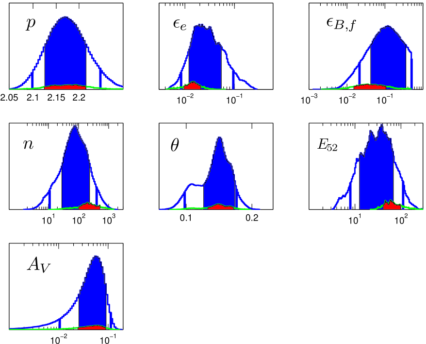
Figure 3: Posterior distribution of all parameters for model (A), which excludes data related to the flaring activity at $t\approx 470$ s: $p$, the power-law index of the electron energy distribution; $\epsilon_{e}$, the electron equipartition parameter; $\epsilon_{B,f}$, the magnetic field equipartition parameter in the forward shock; $n$, the circumstellar density in units of $\rm cm^{-3}$; $\theta$, the opening half-angle before jet break; $E_{52}$, the isotropic-equivalent kinetic energy in units of $10^{52}$ ergs; and $A_{V}$, the dust extinction of the host galaxy. In each plot, the shaded blue region delimits the 1-$\sigma$ (68.2%) confidence range, and the vertical lines indicate the 90%-confidence range. The green color indicates the posterior distribution of the parameters for models having $\gamma_{m}<2.1$ at $t=10^{7}$ s, with the red lines indicating 1-$\sigma$ confidence ranges, and the height of the distribution magnified by a factor of five for clarity; these model realizations correspond to roughly 1.5% of the total.

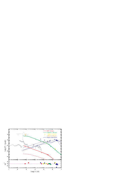
Figure 4: Top: Theoretical light curves (solid lines) corresponding to the best-fit parameters for model (A), which excludes data related to the flaring activity at $t\approx 470$ s. Best-fit model parameters are $p=2.152,\epsilon_{e}=0.031,\epsilon_{B,f}=0.198,n=84.4\,{\rm cm^{-3}},\theta=0.128,E_{52}=22.4,A_{V}=0.0343$ mag. We have shown all the available data on the plot. If the data point is used in the fitting, it is plotted with a bright color, otherwise it is plotted in grey. To illustrate the effects of different densities for model (A), we show additional light curves. The dashed lines correspond to $n=10^{3}\ {\rm cm^{-3}}$, with marginalized best-fit parameters of $p=2.25,\epsilon_{e}=0.019,\epsilon_{B,f}=0.043,\theta=0.182,E_{52}=44,A_{V}=0.0426$ mag, and with reduced chi-squared value $46.1/26=1.77$. The dotted lines correspond to $n=10\ {\rm cm^{-3}}$, with marginalized best-fit parameters of $p=2.19$, $\epsilon_{e}=0.014$, $\epsilon_{B,f}=0.078$, $\theta=0.098$, $E_{52}=50.5$, $A_{V}=0.064$ mag, and reduced chi-squared value $42.1/26=1.62$. All light curves show the total of synchrotron and inverse Compton emission; optical and near-infrared data have been converted to $J$-band flux densities for clarity in plotting. For the best-fit model only, we plot the contribution to the X-ray flux from inverse Compton emission separately, as the red dash-dotted line. Bottom: The chi-squared contribution from each data point. Positive values indicate that the best-fit model underestimates the flux, and negative values indicate that it overestimates the flux.

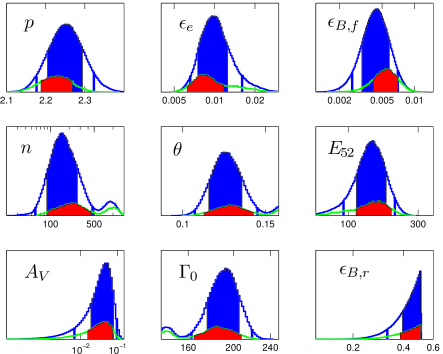
Figure 5: Posterior distribution of all parameters in model (B), in which the flares at $t\approx 470$ s are considered to be emission from the reverse shock regions: $p$, the power-law index of the electron energy distribution; $\epsilon_{e}$, the electron equipartition parameter; $\epsilon_{B,f}$, the magnetic field equipartition parameter in the forward shock; $n$, the circumstellar density in units of $\rm cm^{-3}$; $\theta$, the opening half-angle before jet break; $E_{52}$, the isotropic-equivalent kinetic energy in units of $10^{52}$ ergs; $A_{V}$, the dust extinction of the host galaxy; $\Gamma_{0}$, the initial Lorentz factor of the outflow; and $\epsilon_{B,r}$, the magnetic field equipartition parameter in the reverse shock. The shaded blue region delimits the 1-$\sigma$ range ($68.2\%$), and the region included within the vertical blue lines corresponds to $90\%$-confidence level. The green color indicates the region for $\gamma_{m}<2.1$ (the red color corresponds to 1-$\sigma$ confidence range), which is around $4.7\%$ of the total trials; ; its height has been magnified by a factor of five for clarity.

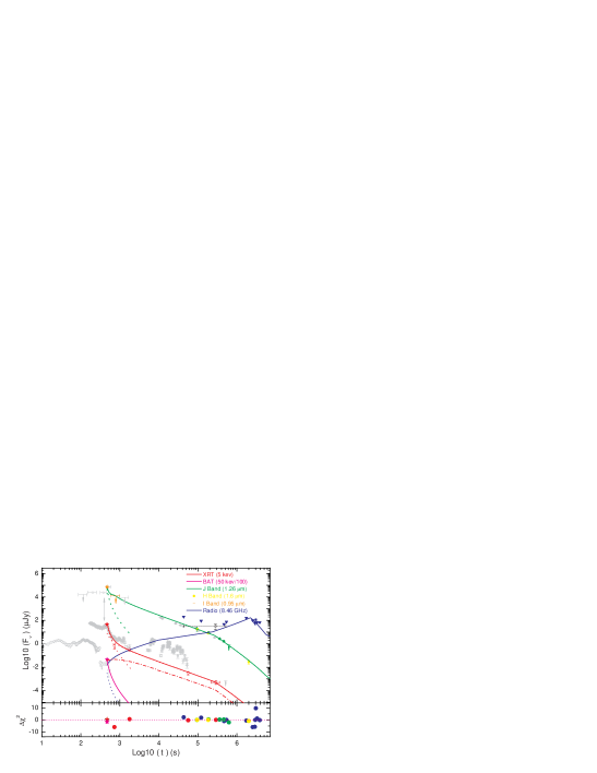
Figure 6: Top: Theoretical light curves (solid lines) corresponding to the best-fit parameters in model (B), in which the flares at $t\approx 470$ s are considered to be emission from the reverse shock regions. Best-fit model parameters are: $p=2.243$, $\epsilon_{e}=0.0084$, $\epsilon_{B,f}=5.7\times 10^{-3}$, $n=212.4\,{\rm cm^{-3}}$, $\theta=0.126$, $E_{52}=147$, $A_{V}=3.18\times 10^{-2}$ mag, $\Gamma_{0}=183.6$, and $\epsilon_{B,r}=0.50$. The dotted lines indicate the separate flux contributions from the reverse and forward shocks (reverse shock emission is distinguished by its fast decay at early times). The solid lines indicate the total model flux, with the red dash-dotted line showing the contribution to the X-ray flux from inverse Compton emission, which is relatively unimportant compared to the synchrotron component. All optical and near-infrared data have been converted to $J$-band flux densities for clarity in plotting; underlying model calculations use the various observed frequencies directly. Radio, $I$-band, $J$-band, $H$-band, X-ray, and BAT data are plotted in blue, orange, green, yellow, red, and magenta, respectively, as indicated in the plot legend. Bottom: The contribution to the total (best-fit) model chi-squared for each data point. Positive values indicate that the model underestimates the flux, and negative values indicate that it overestimates the flux.

4 ANALYSIS OF THE RESULTS

4.1 $J$-Band Light-Curve and IC Suppression

The shift of the afterglow starting time to the epoch $t_{0}^{{}^{\prime}}\sim 402$ seconds modifies the analysis and the interpretation of the early afterglow in model (B), but this should not affect the late-time afterglow light curve evolution, which should be similar to the one for model (A). Thus the discussion below will be focused on the light curve of model (A), and where there are differences, these are pointed out.

Haislip et al. (2006) have fitted their collection of NIR data, and find that between 3 hours and 0.5 days after the burst, the fading of the afterglow can be fitted by a power law of index $\alpha=1.36^{+0.07}_{-0.06}$, while after 0.5 days the fading appears to slow down to a temporal index of $0.82^{+0.21}_{-0.08}$. At $t=10.6$ hours (0.44 days), the spectral index is $\beta_{o}=1.25^{+0.15}_{-0.14}$. A single power-law decay is ruled out at 3.7$\sigma$ confidence. Tagliaferri et al. (2005) have extended datasets whose observation time reaches up to 7 days after the burst, and fit the lightcurve with a smoothly-broken power law. The fit gives $\alpha_{1}=0.72^{+0.15}_{-0.20}$, $\alpha_{2}=2.4\pm 0.4$, and $t_{b}=2.6\pm 1.0$ days. In addition, the spectral index at $t=1.155$ days is calculated to be $\beta=1.25\pm 0.25$ or $\beta=1.2\pm 0.3$ by two slightly different fitting codes. Thus, based only on the observations in the optical/NIR bands, we can divide the light curve into 3 segments: (D) $t<0.5\ {\rm days}$: the afterglow decays as a power-law with index of $1.36^{+0.07}_{-0.06}$; (E) $0.5\ {\rm days}<t<1.6\ {\rm days}$: the light curve is relatively flat, decaying as a power-law with index $\alpha\approx 0.82$; and (F) $t>1.6\ {\rm days}$: the light curve decays with an index of $2.4\pm 0.4$ (see Fig. 1).

Wei et al. (2006) have argued that the fast decay during stage (D) represents the normal afterglow, and the flattening at stage (E) is caused by energy injection. Then the stage (F) would indicate a return to the normal afterglow evolution. Here, however, we have presented a different interpretation for the stages (D) and (E). The flux at stage (D) is considered to be suppressed by the inverse Compton interaction between electrons in the forward shock and X-ray flare photons, while the flux in stage (E) is the normal flux without external inverse Compton process. This is motivated by the argument of Wang et al. (2006) suggesting that the X-ray flare photons can interact with the electrons in the forward shock regions via inverse Compton scattering. The origin of the late-time X-ray flares is unknown, although a widely-held view is that they are due to the internal shocks from late time engine activity. Since these X-ray photons would be coming, in this view, from a region different from (and behind) the forward shock, we call this Inverse Compton (IC) process an “external IC process.” In this case, the external IC process will contribute significantly to the cooling of the forward shock electrons, since the flare luminosity is much larger than the forward shock (afterglow) luminosity, and the Compton parameter is determined by the ratio of those two luminosities. If the total radiated energy at a given time is constant, when the energy radiated via the inverse Compton process increases, the synchrotron radiation should decrease. In effect, this can be viewed as the synchrotron radiation having been suppressed by the inverse Compton process. Since the $J$-band luminosity at this time is dominated by synchrotron radiation, the observed flux would become smaller in the presence of strong external IC processes. At the end of the flare, the external inverse Compton suppression disappears, and the synchrotron radiation can then return to its normal course.

If we assume that the averaged luminosity ratio between the flare and the forward shock in the X-ray is $k=L_{\rm IC,fl}/L_{\rm syn,f}$ (“fl” is the flare and “f” denotes the forward shock), following the similar definition for the Compton parameter which is the ratio of the IC luminosity to the synchrotron luminosity $Y_{\rm SSC}=L_{\rm IC,f}/L_{\rm syn,f}=(\eta\epsilon_{e}/\epsilon_{B})^{1/2}$ where the subscript “SSC” indicates the self-Compton scattering process (Sari & Esin 2001), we can get the new Compton parameter, considering the external IC process, as $Y_{\rm IC,fl}=L_{\rm IC,total}/L_{\rm syn,f}=[(L_{\rm IC,fl}+L_{\rm IC,f})/L_{\rm syn,f}]=[(k+1)\eta\epsilon_{e}/\epsilon_{B}]^{1/2}$. We can see an additional factor of $(k+1)^{1/2}$ contributes to the Compton parameter for the external IC process compared with the Compton parameter for the usual SSC case. Because normally the parameter $k\gg 1$, we expect $Y_{\rm IC,ext}>Y_{\rm SSC}$. For the fast-cooling case, $\eta=1$, so we have $Y_{\rm IC,fl,fast}=[(k+1)\epsilon_{e}/\epsilon_{B}]^{1/2}$ and $Y_{\rm SSC,fast}=(\epsilon_{e}/\epsilon_{B})^{1/2}$. The IC process will affect the synchrotron radiation, and change the cooling frequency $\nu_{c}$ for synchrotron radiation and the observed flux $F_{\nu}\propto\nu_{c}^{1/2}$. For synchrotron radiation, $\nu_{c}\propto(1+Y)^{-2}$ and the external IC process will lead to a much lower cooling frequency $\nu_{c}$ due to an increase in the value of the Compton parameter. During the time period of stage (D) in Fig. 1, the electrons are in the fast-cooling regime, $\nu_{c}<\nu_{m}<\nu_{o}$, where $\nu_{o}$ is the observing frequency, so that the ratio of the flux without external IC to the flux with external IC is $\hat{S}={F_{\rm no}/F_{\rm IC}}=(1+Y_{\rm IC,fl,fast})/(1+Y_{\rm SSC,fast})\approx(k+1)^{1/2}$, where $F_{\rm IC}$ is the flux with external IC process considered and the flux without IC is $F_{\rm no}=(1+Y_{\rm IC,ext})/(1+Y_{\rm SSC})F_{\rm IC,ext}\sim(k+1)^{1/2}F_{\rm IC}$. Therefore, the observed flux in the optical/NIR band during section (D) should be multiplied by a factor $[(1+k)^{1/2}]$ to recover the flux that would be observed without IC suppression effects.

We can estimate the required luminosity ratio from the observed suppression factor. Taking the power-law index for the electron energy distribution to be $p=2.2$, the theoretically expected temporal index is $\alpha=(3p-2)/4=1.15$ for $\nu_{o}>(\nu_{c},\nu_{m})$, the expected regime for the optical afterglow during stage (E). Then we can extrapolate the optical lightcurve back from $t=1.92\times 10^{5}$ s (where the flux is $f=9.14\pm 1.75$$\mu$Jy) to the observer time $t=2.7\times 10^{4}$ s, where the observed flux is $f\approx 55$ $\mu$Jy. This theoretical flux, in the absence of the external IC process, will be $9.14\cdot(1.92\times 10^{5}/2.7\times 10^{4})^{1.15}\simeq 81.0$ $\mu$Jy. Thus, the flux will be suppressed by a factor of $\hat{S}\sim 1.6\approx(1+k)^{1/2}$. From the observational point of view, we invert this problem and solve for $k$, deriving $k\approx 1.6$.

Apparently, compared to the mean observed luminosity ratio between the flares and the forward shock, $F_{\rm fl}/F_{\rm fs}\lower 4.0pt\hbox{$\buildrel>\over{\sim}$}10$ (see Fig. 1), this indicates within our picture that only a small fraction of the flare photons have interacted with the electrons in the afterglow. A possible explanation could be that the anisotropic distribution of the incoming flare photons in the comoving frame of the afterglow shock (Wang et al. 2006). This resultsing more head-on scattering which reduces the IC interaction. Therefore, the suppression is relatively small and the optical flux is only affected to a reduce degree.

4.2 Radio Light-curve

GRB 050904 shows several similarities with GRB 990123, including a large isotropic-equivalent gamma-ray energy and a very bright optical flash. In GRB 990123, the radio emission was observed to peak at $t=1$ day in the observer frame, and this emission was interpreted as the radio emission from the reverse shock (Sari & Piran 1999). Given the important role of the reverse shock in our model (B) of GRB 050904, it is interesting to consider its radio emission. However, our estimates indicate that the reverse shock radio emission at early time would be suppressed by the large circumburst density in our model, so that we would not expect to observe a bright radio flare. In Fig. 6, we have plotted the reverse shock radio emission as a dotted blue line starting from $t=470$ s, while the solid blue line shows the combined radio emission from both the forward shock and the reverse shock; as can be seen, the emission from the reverse shock is negligible.

In Fig. 6, there is one averaged radio data point centered at $t\sim 2\times 10^{5}$ seconds and $f_{\nu}\sim 30\ {\rm\mu Jy}$ (indicated with dashed lines ) based on the average of multiple VLA observations spanning $\sim 6$ days (see Fig. 2 of Frail et al. 2006). Given the large dynamic range in time, we consider this data point as an upper limit of the radio emission during that period. We can see that our best-fit radio light curve for the forward shock in both models (A) and (B) fits accommodates this upper limit reasonably well, along with the other data points.

4.3 Density and Energy Constraints

The density obtained in our fit, $n\approx 84.4$ cm^-3 for model (A) and $n\approx 212.4$ cm^-3 for model (B), is smaller than the $n=680$ cm^-3 density derived by Frail et al. (2006). Investigating our model fits, we find that the discrepancy arises because their model peaks later in the radio than ours. Referring to the posterior distribution for the density parameter in Figs. 3 and 5, we find that the most likely range (90%-confidence) for density is from 26 to 273.4 cm^-3 for model (A) and from 87.8 to 270.6 cm^-3 for model (B). On the other hand, the light curves for different densities demonstrate that there is no big noticeable affect of these density changes on the X-ray and optical/NIR lightcurves.

The radio observations thus provide the best frequency for density constraints, and fail to provide a tight constraint mainly because of the lack of data (measurements) late times.

With regards to the circumburst density, we note that Kawai et al. (2006) observed the spectrum and detected in it fine structure lines including $\rm SiII^{*}$, which were taken to imply an electron density of up to $10^{2.3\pm 0.7}\ {\rm cm^{-3}}$. The density obtained from the spectral lines would thus be consistent with our best-fit value for the density, and suggest that the observed lines formed in region similar to that hosting the GRB itself. However, we note that several recent papers (Berger et al. 2005; Prochaska et al. 2006) have suggested that these fine-structure transitions in GRB afterglows are excited by radiative processes, rather than collisions, which would make the density constraint irrelevant.

An important check on our model results, pointed out by Frail et al. (2006), is to estimate the X-ray luminosity from the X-ray light curve at some fiducial time (usually at $t=10$ hours). At $t=3.36$ days, the observed flux over the XRT energy range is $\sim 2.1\times 10^{-14}\ {\rm erg\ s^{-1}\ cm^{-2}}$. Calculating back to $t\sim 10$ hours for the afterglow flux from synchrotron radiation, the predicted flux is $f\sim 2.8\times 10^{-13}\ {\rm erg\ s^{-1}\ cm^{-2}}$. Therefore the X-ray luminosity should be $L_{X,{\rm iso}}=4\pi D_{L}^{2}f(1+z)^{-\alpha+\beta-1}\sim 1.66\times 10^{46}\ {\rm erg\ s^{-1}}$, and the geometrically-corrected X-ray luminosity we find is different from and significantly lower than theirs. The reason for this is that when they calculate the isotropic-equivalent energy, they appear not to have included the $k$-correction factor $(1+z)^{-\alpha+\beta-1}$. Berger et al. (2003) also appear not to have included the $k$-correction factor when doing statistics on the isotropic-equivalent and geometrically-corrected X-ray luminosity. Here we do the statistics again after putting the correction, and find that the geometrically-corrected X-ray luminosities are still clustered, but the peak value has shifted down to $L_{X,p}\sim 10^{44}{\rm erg/s}$, reduced by a factor of five.

Once we have obtained the X-ray luminosity, we can estimate the kinetic energy with the best fitting parameters and the observed spectral index. In model (A), we have best fitting parameters $\epsilon_{e}=0.0309$, $\epsilon_{B,f}=0.198$ , $\beta\sim 1$, $p=2.152$, and $\alpha=(3p-2)/4$. From the equation D4 in the appendix, we have $E_{52}\simeq 24.4$, which is consistent with the kinetic energy derived from the fit, $E_{K}=22.4$. This is not surprising since the formula in the appendix is only a shortcut to obtain the kinetic energy. In model (B), we have the best fitting parameters $\epsilon_{e}=8.4\times 10^{-3}$, $\epsilon_{B,f}=5.7\times 10^{-3}$ , $\beta\sim 1$, $p=2.243$, and $\alpha=(3p-2)/4$, and similarly we obtain $E_{52}\simeq 148$. After considering the $k$-correction factor for the X-ray luminosity by Frail et al. (2006), we can re-estimate the kinetic energy as $E_{52}\simeq 230$ with the parameters $\epsilon_{e}=0.02$, and $\epsilon_{B}=0.015$, which is 3 times larger than their best-fit kinetic energy $E_{52}\simeq 88$.

Considering our estimated opening half-angles of $\theta\simeq 0.13$ for both models (A) and (B), we can calculate the geometrically-corrected X-ray luminosity for GRB 050904 to be $L_{X}=L_{X,{\rm iso}}\times\theta^{2}/2\approx 1.40\times 10^{44}\ {\rm erg\ s^{-1}}$, which falls within the corrected luminosity range of low-redshift GRBs (Berger et al. 2003).

We now calculate the geometrically-corrected kinetic energy. Our best-fit opening half-angle is $\theta\simeq 0.13$ for both models, and the fitted kinetic energy for model (A) and (B) is $2.24\times 10^{53}$ ergs and $1.47\times 10^{54}$ ergs, so the geometrically-corrected kinetic energy will be $1.84\times 10^{51}$ ergs and $1.17\times 10^{52}$ ergs for models (A) and (B), respectively. Broadband modeling of 10 low-redshift bursts indicated that the geometrically-corrected kinetic energies of two were anomalously high, $2\times 10^{51}$ ergs, approximately 10 times higher than for the other eight GRBs (Panaitescu & Kumar 2002). Our geometrically-corrected kinetic energy for model (A) is comparable to those anomalously-large kinetic energies seen from low-redshift GRBs. The kinetic energy of model (B), on the other hand, is significantly larger even than this. Both models yield a relatively large kinetic energy has been obtained for GRB 050904. GRB 050904 thus suggests that bursts at high redshift are somehow able to tap into a higher-energy reservoir than the low-redshift events.

4.4 Burst Energetics and Efficiency

The radiated isotropic-equivalent gamma-ray energy for GRB 050904 is $6.6\times 10^{53}<E_{\gamma,{\rm iso}}<3.2\times 10^{54}$ ergs (Cusumano et al. 2006). If the isotropic-equivalent kinetic energy for the afterglow of GRB 050904, as we concluded in case (A), is $2.24\times 10^{53}$ ergs, we can estimate the GRB efficiency as $\zeta=E_{\gamma,{\rm iso},52}/(E_{\gamma,{\rm iso},52}+E_{52})$ (Lloyd-Ronning & Zhang 2004), which is $74.7\%<\zeta<93.5\%$ for GRB 050904. If the isotropic-equivalent kinetic energy of the afterglow, as in case (B), is $1.47\times 10^{54}$ ergs, then the corresponding GRB efficiency is roughly $31.0\%<\zeta<68.5\%$. In either case, this indicates that GRB 050904 has a high efficiency; however, such high efficiencies are not unique. Lloyd-Ronning & Zhang (2004) found that a substantial number of GRBs have high efficiency. For some bursts like GRB 990705, the inferred efficiency even reaches up to $99\%$. Fan & Piran (2006) have shown that the inferred efficiency can be reduced when inverse Compton effects are taken into account (see also Granot et al. 2006). Even so, there are still several bursts which have a high observed efficiency, for example, $94\%$ for GRB 050315 and $80\%$ for GRB 050416 (Zhang et al. 2007).

5 Discussion

The extreme interest in GRB 050904 has motivated several groups to analyze the burst data and suggest interpretations. These works fall into two categories: (1) Comparing the properties of GRB 050904 with other bursts; and (2) Making fits to the GRB 050904 data either in the framework of internal shock or external shock models. We give a brief description below of the work of other groups and mention key differences between their work and ours.

In category (1), Kann et al. (2007) made a composite $J$-band light curve starting from $2\times 10^{-3}$ days to $\sim 23$ days. After applying extinction correction, they shifted GRB 050904 as well as lower-redshift bursts to $z=1$, and made a comparison of afterglow lightcurves. They found that GRB 050904 is much brighter than other GRBs at early times, but of roughly equal brightness at late times. Thus they conclude that GRB 050904 most likely is still a normal GRB.

The other analyses are all in category (2). Zou et al. (2006) argued that GRB 050904 is a burst with extremely long central engine activity. They put all the observed data within the framework of the internal shock model. By contrast, we only treat the first several hundred seconds (BAT) as internal shock activity in our model (corresponding to the stages (A) and (B) for model (A), and stage (A) for model (B) in Fig. 1). The late-time X-ray flares between $6\times 10^{3}$ and $6\times 10^{4}$ seconds may be due to internal shock, but we have interpreted portions of this X-ray emission as being due to the forward-shock afterglow.

Wei et al. (2006) argued that the $t\approx 470$ s flare is from internal shocks on the basis of its fast decay (the temporal index is $\alpha\approx 8.8$ relative to the trigger time) and also because the optical-to-X-ray emission of the flare cannot be described by a synchrotron radiation model (Boër et al. 2006). They made fits to all the available $J$-band data. They argue that the slow-decay portion of the lightcurve is due to energy injection. In our model, besides fitting over all the additional bands (X-ray and radio), we propose a new mechanism for the flattening, namely that it is caused by the suppression of the synchrotron radiation by the interaction between the X-ray flare photons and afterglow electrons. Separately, in our model (B), we introduced a new reference time $t_{0}^{{}^{\prime}}$ which flattens the decay index, and allows us to interpret the $t\approx 470$ s optical/X-ray flare as arising in the reverse shock.

Frail et al. (2006) made broadband model fits including the X-ray, NIR/optical, and radio data. The difference with our work is partly that we have used the larger data set that later became available. We have included two X-ray data points as early as $t\sim 10^{3}$ seconds, and we also included the $H$ band data observed $t\sim 23$ days after the burst (Berger et al. 2006). Since most of the other data are concentrated around $t\sim 10^{5}$ seconds, the introduction of these additional X-ray and NIR data have some impact on the final fitting result. The other major difference is that we have freed all the possible parameters and applied the MCMC method for the global fitting, making an efficient exploration of the full parameter space, and providing the posterior distributions (including confidence intervals) for each parameter.

Gendre et al. (2007) argued that the power-law-like decay right after the flare $t\approx 470$ s should be interpreted as forward shock emission. Because the extrapolation of the late time X-ray flux to early times is lower than the observed value, they found that a wind-type environment was favored by the closure relationship for this early-time segment (it should also be noted that their spectral index is smaller than Cusumano et al. (2006)). They propose a density-jump model for the afterglow evolution: before a certain radius, the density goes as $n\propto r^{-2}$ and after that, the density is a constant ISM model. At the transition point a termination shock is formed which lies around $R_{t}\sim 1.8\times 10^{-2}$ pc from the central engine. In our model, we consider the same segment of data, but interpret it differently. We argue that the flux between 600 and 800 seconds arises from the combination of three sources: high-latitude emission of the prompt emission, flux from the flare, and forward shock emission. Reviewing the data closely, we see that actually there are two other small flares between 800 and 2000 seconds, so the data around $t\sim 1500$ seconds has the contribution from the flares and the forward shock (see Fig. 2). Once we subtract the flare contribution from the observed data, we argue, the forward shock contribution is what remains. And in fact, we find that an extrapolation of the late-time flux to early times is consistent with this flare-subtracted early-time flux.

There remain some substantial differences in parameter values between the two models that we have presented. For example, the most likely value for $\epsilon_{B,f}$ in model (A) is roughly $\sim 0.1$, but the most likely value for $\epsilon_{B,f}$ in model (B) is around $5\times 10^{-3}$. It turns out that the main difference lies in the optical flux at early times. We take as an example the $J$-band light curve for the best fitting parameter set in model (A). The flux slowly decays with an index of $\alpha\approx 0.5$ before $t\sim 2\times 10^{3}$ and then follows a faster decay with a temporal index of $\alpha\approx 1.1$ after $t\sim 2\times 10^{3}$. The break at $t\sim 2\times 10^{3}$ seconds is caused by the crossing of the electron’s typical frequency $\nu_{m}$ through the optical observing frequency. Since we have $\nu_{m}\propto\epsilon_{B,f}^{1/2}$, then the smaller $\epsilon_{B,f}$, the smaller the typical frequency, therefore the earlier the crossing time. The fit in model (B) requires an earlier break than in model (A), so a smaller value of $\epsilon_{B,f}$ is expected in model (B). Since the observed flux from the forward shock is the same in both models, we expect a higher kinetic energy in model (B). Similarly, at the deceleration time, the reverse shock flux is larger than that from the forward shock, so a larger $\epsilon_{B,r}$ is expected in the reverse shock.

We notice that in both our models we find a small value for $\epsilon_{e}$, e.g., the best fitting $\epsilon_{e}=3.1\times 10^{-2}$ for model (A) and $\epsilon_{e}=8.4\times 10^{-3}$ for model (B). Considering the radiative correction factor $R=(t/t_{0})^{17\epsilon_{e}/48}$ (where $t_{0}$ is the deceleration time, and we set $t_{0}=300$ seconds for model (A) and $t_{0}=470$ seconds for model (B)), that is, the amount by which the kinetic energy at time $t$ is reduced by comparison to the kinetic energy at time $t_{0}$, we find $R=1.07$ for model (A) and $R=1.02$ for model (B) at $t=1.0\times 10^{5}$ seconds after the burst. Therefore, the radiative losses are mild in either case, consistent with our assumption that the afterglow evolves in an adiabatic fashion.

Our fitting results also show that the host galaxy dust extinction is quite small, $A_{V}\sim 0.1$ mag or even smaller, consistent with the results from Kann et al. (2007). They applied several different dust models (MW, LMC and SMC) over the composite $J$-band, and all the models suggested zero or negligible extinction. In the context of GRB 990123, it was suggested that the negligible extinction to the burst was the result of dust destruction by the strong burst and early-afterglow emission (Kann et al. 2006).

6 CONCLUSIONS

In this paper we have performed the most extensive multiband analysis so far of the GRB 050904 afterglow. We have considered two scenarios: (A) Only forward shock emission is considered, and the flares peaking at $t\approx 470$  after the burst are assumed to be due to internal shocks (or are otherwise independent of the afterglow); and (B) The NIR and X-ray flares at $t\approx 470$ s are ascribed to emission from the reverse shock – when the ejecta has swept up enough material and starts to decelerate, the synchrotron radiation in the reverse shock produces the optical flare, and the self-Compton scattering of synchrotron photons generates the flare observed in the XRT and BAT energy bands.

Combining the early afterglow data with late-time observations in the X-ray, optical and radio, and using a Markov chain Monte Carlo method, we present a full characterization of the posterior distributions (including confidence intervals) for the various parameters of our model fits. Our best-fit parameter values for model (A) are $p=2.152$, $\epsilon_{e}=0.309$, $\epsilon_{B,f}=0.198$, $n=84.4$ cm^-3, $\theta=0.128$, $E_{52}=22.4$, and $A_{V}=0.0343$ mag, with a reduced chi-squared value of $36.2/26\approx 1.39$. Our best-fit parameter values for model (B) are $p=2.243$, $\epsilon_{e}=0.0084$, $\epsilon_{B,f}=5.7\times 10^{-3}$, $n=212.4$ cm^-3, $\theta=0.126$, $E_{52}=147$, $A_{V}=3.18\times 10^{-2}$ mag, $\Gamma_{0}=183.6$, and $\epsilon_{B,r}=0.50$, with a reduced chi-squared value of $53.0/28\approx 1.89$. Note that the subscripts $r$ and $f$ refer to the reverse shock and forward shock respectively, $\epsilon_{B,f}=\epsilon_{B,r}/R_{B}^{2}$, and we have assumed $\epsilon_{e,f}=\epsilon_{e,r}$.

We have compared the density, the geometrically-corrected kinetic energy and the X-ray luminosity at $t=10$ hours derived here for our two models of GRB 050904 against those values for other bursts, as derived from afterglow modeling. The results for both models show that although the X-ray luminosity of GRB 050904 falls within the range for low-redshift GRBs, the density and geometrically-corrected kinetic energy are both above the typical values for low-redshift GRBs, which suggests that GRB 050904 may be a member of a distinct population of high-redshift, higher kinetic-energy bursts, whose properties differ from those of low-redshift GRBs. A clear preference between our (A) and (B) models is hard to establish at present, since there is only one high-redshift GRB known. One would like access to several more high-redshift GRB observational datasets before attempting to discriminate between the two models.

It is estimated that $\sim 7\%-40\%$ GRBs are located at $z>5$ (Jakobsson et al. 2006), and detection rate simulations by Gou et al. (2004) indicate that Swift could detect GRBs out to redshift $z\sim 30$, if they are present. Bromm & Loeb (2006) also predict that $10\%$ of the Swift GRBs originate at $z>5$. It appears that one can realistically expect a handful (5 to 10) of additional high-redshift GRB detections with rapid follow-up in the next few years of the Swift mission. In this case, the consistent application of MCMC methods, as used here, will lead efficiently to a set of statistically well-quantified, posterior parameter distributions and confidence intervals. This would enable a statistically meaningful comparison of high-redshift and low-redshift GRB parameters, which might well lead us to a definite understanding of the physics and environments of GRBs as a function of redshift, up to the highest redshifts detected. This would also have a substantial impact on the study of the large scale structure and star formation processes throughout the Universe, and the properties of the cosmic reionization at $z\sim 6$.

Appendix A Self-Absorption Frequency

Once we consider radio emission in our afterglow models, the self-absorption frequency becomes an important parameter to consider. Below we give the expressions for the self-absorption frequency in the different regimes.

If we assume that the electron distribution follows a power law $N(\gamma_{e})=N_{\gamma}\gamma_{e}^{-p}$ where $\gamma_{1}<\gamma_{e}<\gamma_{2}$, then the self-absorption coefficient for the various possible regimes is (Wu et al. 2003):

$$k_{\nu}=\frac{q_{e}}{B}N_{\gamma}\left\{\begin{array}[]{ll}c_{1}\gamma_{1}^{-(p+4)}\left(\frac{\nu}{\nu_{1}}\right)^{-5/3}&\nu\ll\nu_{1}\\ c_{2}\gamma_{1}^{-(p+4)}\left(\frac{\nu}{\nu_{1}}\right)^{-(p+4)/2}&\nu_{1}\ll\nu\ll\nu_{2},\\ c_{3}\gamma_{2}^{-(p+4)}\left(\frac{\nu}{\nu_{2}}\right)^{-5/2}e^{-\nu/\nu_{2}}&\nu\gg\nu_{2}\end{array}\right.$$ (A1)

where $c_{1}=\frac{32\pi^{2}}{9\times 2^{1/3}\Gamma(1/3)}\frac{p+2}{p+2/3}$, $c_{2}=\frac{2\sqrt{3}\pi}{9}2^{p/2}(p+\frac{10}{3})\Gamma(\frac{3p+2}{12})\Gamma(\frac{3p+10}{12})$, $c_{3}=\frac{2\sqrt{6}\pi^{3/2}}{9}(p+2)$, $\nu_{1}$ and $\nu_{2}$ are the typical synchrotron frequencies of electrons with the Lorentz factor $\gamma_{1}$ and $\gamma_{2}$, respectively, and $\Gamma(x)$ is the Gamma function.

Following the definition of $\kappa_{\nu}(\nu_{a})l=1$ for the self-absorption frequency (where $l=R/\Gamma$ is the thickness of the shell), we can find the self-absorption for the forward shock region. The self-absorption frequency for the reverse shock has a similar form, with the difference that the quantities specific to the forward shock region should be replaced with those specific to the reverse shock.

Fast Cooling: $\nu_{a}<\nu_{c}<\nu_{m}$,

$$\nu_{a}^{(1)}=\nu_{c}\left({c_{1}q_{e}n_{0}R\over 3B\gamma_{c}^{5}}\right)^{3/5}\\$$ (A2)

where the superscript “$i$” denotes the different regimes.

Fast Cooling: $\nu_{c}<\nu_{a}<\nu_{m}$,

$$\nu_{a}^{(2)} = \nu_{c}\left({c_{2}q_{e}n_{0}R\over 3B\gamma_{c}^{5}}\right)^{1/3}$$ (A3)

$$\nu_{a}^{(2)} = \nu_{c}^{4/9}(\nu_{a}^{(1)})^{5/9}$$ (A4)

Fast Cooling: $\nu_{c}<\nu_{m}<\nu_{a}$,

$$\nu_{a}^{(3)} = \nu_{m}\left({c_{2}q_{e}n_{0}R\gamma_{c}\over 3B\gamma_{m}^{6}}\right)^{2/(p+5)}$$ (A5)

$$\nu_{a}^{(3)} = [(\nu_{a}^{(1)})^{10/3}\nu_{c}^{8/3}\nu_{m}^{p-1}]^{1/(p+5)}$$ (A6)

Slow Cooling: $\nu_{a}<\nu_{m}<\nu_{c}$

$$\nu_{a}^{(4)}=\nu_{m}\left({c_{1}(p-1)q_{e}n_{0}R\over 3B\gamma_{m}^{5}}\right)^{3/5}\\$$ (A7)

We notice that $\nu_{a}^{4}/\nu_{a}^{1}=(p-1)^{3/5}(\nu_{c}/\nu_{m})^{1/2}$. To keep the continuity of the flux while the afterglow transits from the fast-cooling regime to the slow-cooling regime, we divide $\nu_{a}^{(4)}$ by a factor of $(p-1)^{3/5}$.

Slow Cooling: $\nu_{m}<\nu_{a}<\nu_{c}$,

$$\nu_{a}^{(5)}=\nu_{m}\left({c_{2}(p-1)q_{e}n_{0}R\over 3B\gamma_{m}^{5}}\right)^{2/(p+4)}$$ (A8)

$$\nu_{a}^{(5)}=[(\nu_{a}^{(4)})^{10}\nu_{m}^{(3p+2)}]^{1/(3(p+4))}$$ (A9)

Slow Cooling: $\nu_{m}<\nu_{c}<\nu_{a}$,

$$\nu_{a}^{(6)}=\nu_{c}\left({c_{2}(p-1)q_{e}n_{0}R\gamma_{m}^{p-1}\over 3B\gamma_{c}^{p+4}}\right)^{2/(p+5)}$$ (A10)

$$\nu_{a}^{(6)}=[(\nu_{a}^{(1)})^{10/3}\nu_{c}^{8/3}\nu_{m}^{p-1}]^{1/(p+5)}$$ (A11)

it can be shown that the self-absorption frequency in the regime $\nu_{m}<\nu_{c}<\nu_{a}$ has the same form as that for the fast-cooling case, $\nu_{c}<\nu_{m}<\nu_{a}$.

Because the observer time, $t_{obs}$, at $z=0$ is connected to the time in the source frame, $t_{s}$, at redshift $z$ by the relation $t_{obs}=(1+z)t_{s}$, we have the redshift dependence for main characteristic quantities: the shock radius $R\propto t_{s}^{1/4}\propto(1+z)^{-1/4}$, the shock Lorentz factor $\Gamma\propto t_{s}^{-3/8}\propto(1+z)^{3/8}$, the magnetic field $B\propto\Gamma\propto(1+z)^{3/8}$, the typical Lorentz factor $\gamma_{m}\propto\Gamma\propto(1+z)^{3/8}$, the cooling Lorentz factor $\gamma_{c}\propto t_{s}^{-1}\Gamma^{-3}\propto(1+z)^{-1/8}$. In addition, we have $\nu_{m}\propto(1+z)^{1/2}$ and $\nu_{c}\propto(1+z)^{-1/2}$ (see Eqn. 2.4.1). Substituting these dependence into the relations for the self-absorptions above, the redshift dependence for the self-absorptions is $\nu_{a}^{(1)}\propto(1+z)^{-1/2},\nu_{a}^{(2)}\propto(1+z)^{-1/2},\nu_{a}^{3}\propto(1+z)^{(p-7)/[2(p+5)]},\nu_{a}^{(4)}\propto(1+z)^{-1},\nu_{a}^{(5)}\propto(1+z)^{(p-6)/[2(p+4)]}$, and $\nu_{a}^{(6)}=\nu_{a}^{(3)}\propto(1+z)^{(p-7)/[2(p+5)]}$.

Appendix B Inverse Compton Spectrum

As described by Sari & Esin (2001), the inverse Compton flux can be calculated from the following double integral:

$$f_{\nu}^{IC}=R\sigma_{T}\int_{\gamma_{m}}^{\infty}d\gamma N(\gamma)\int_{0}^{x_{0}}dxf_{\nu_{s}}(x)\\$$ (B1)

where $N(\gamma)$ is the electron distribution in the shocked shell, $f_{\nu_{s}}(x)$ is the seed photon flux, and $x$ is defined as $x=\nu/4\gamma^{2}\nu_{s}$ where the subscript “$s$” denotes the seed photon.

B.1 $\nu_{c}<\nu_{a}<\nu_{m}$

The distribution of seed photons is described by the synchrotron spectrum, a broken power law with the characteristic quantities (Sari et al. 1998). Then the inner integral in Eqn. (B1) gives:

$$I=\left\{\begin{array}[]{l@{\quad\quad}l}I_{1}\simeq\frac{5}{3}f_{max}x_{0}\left(\frac{\nu}{4\gamma^{2}\nu_{a}^{(2)}x_{0}}\right),&\nu<4\gamma^{2}\nu_{a}^{(2)}x_{0}\\ I_{2}\simeq\frac{2}{3}f_{max}x_{0}\left(\frac{\nu}{4\gamma^{2}\nu_{m}x_{0}}\right)^{\frac{-1}{2}},&4\gamma^{2}\nu_{a}^{(2)}x_{0}<\nu<4\gamma^{2}\nu_{m}x_{0}\\ I_{3}\simeq\frac{2}{(p+2)}f_{max}x_{0}\left(\frac{\nu_{m}}{\nu_{a}^{(2)}}\right)\left(\frac{\nu}{4\gamma^{2}\nu_{m}x_{0}}\right)^{-\frac{p}{2}},&\nu>4\gamma^{2}\nu_{m}x_{0}.\end{array}\right.$$ (B2)

The integration over different electron energies again needs to be divided into four different regimes:

$$f_{\nu}^{IC}=R\sigma_{T}$$ (B3)

$$\times \left\{\begin{array}[]{ll}\displaystyle\int_{\gamma_{c}}^{\infty}{d\gamma N(\gamma)I_{1}}+,&\nu<\nu_{a}^{IC};\\ \left[\displaystyle\int_{\gamma_{c}}^{\gamma_{cr}(\nu_{a})}{d\gamma N(\gamma)I_{2}}+\displaystyle\int_{\gamma_{cr}(\nu_{a})}^{\infty}{d\gamma N(\gamma)I_{1}}\right],&\nu_{a}^{IC}<\nu<\nu_{m}^{IC};\\ \left[\displaystyle\int_{\gamma_{c}}^{\gamma_{cr}(\nu_{m})}{d\gamma N(\gamma)I_{3}}+\displaystyle\int_{\gamma_{cr}(\nu_{m})}^{\gamma_{cr}(\nu_{a})}{d\gamma N(\gamma)I_{2}}+\displaystyle\int_{\gamma_{cr}(\nu_{a})}^{\infty}{d\gamma N(\gamma)I_{1}}\right],&\nu_{m}^{IC}<\nu;\\ \end{array}\right.$$ (B7)

Evaluating the integrals in Eqn. (B3), we only keep the dominant terms:

$$f_{\nu}^{IC} \simeq R\sigma_{T}nf_{max}x_{0}$$ (B8)

$$\times \left\{\begin{array}[]{ll}\frac{5}{9}\left(\frac{\nu}{\nu_{a}^{IC}}\right),&\nu<\nu_{a}^{IC}\\ \frac{1}{3}(\frac{\nu}{\nu_{a}^{IC}})^{-1/2}[\log\left(\frac{1}{3}\frac{\nu}{\nu_{a}^{IC}}\right)+\frac{5}{9}],&\nu_{a}^{IC}<\nu<\sqrt{\nu_{m}^{IC}\nu_{c}^{IC}};\\ (\frac{\nu}{\nu_{a}^{IC}})^{-1/2}[\frac{2}{(p+2)(p-1)}+\frac{1}{3}\log\left(\frac{\nu_{m}}{\nu_{a}}\right)+\frac{5}{9}],&\sqrt{\nu_{m}^{IC}\nu_{c}^{IC}}<\nu<4\gamma_{m}^{2}\nu_{a}x_{0};\\ (\frac{\nu}{\nu_{a}^{IC}})^{-1/2}[\frac{2}{(p+2)(p-1)}+\frac{2}{3(p-1)}+\frac{1}{3}\log\left(\frac{\nu_{m}^{IC}}{\nu}\right)],&4\gamma_{m}^{2}\nu_{a}x_{0}<\nu<\nu_{m}^{IC};\\ (\frac{\nu_{m}^{IC}}{\nu_{a}^{IC}})^{-1/2}(\frac{\nu}{\nu_{m}^{IC}})^{-p/2}[\frac{2}{(p+2)(p-1)}+\frac{1}{p+2}\log\left(\frac{\nu}{\nu_{m}^{IC}}\right)+\frac{2}{3(p-1)}],&4\gamma_{m}^{2}\nu_{a}x_{0}<\nu<\nu_{m}^{IC}\end{array}\right.$$ (B14)

B.2 $\nu_{c}<\nu_{m}<\nu_{a}$

$$I=\left\{\begin{array}[]{l@{\quad\quad}l}I_{1}\simeq\frac{2(p+5)}{3(p+2)}f_{max}x_{0}\left(\frac{\nu}{4\gamma^{2}\nu_{a}x_{0}}\right),&\nu<4\gamma^{2}\nu_{a}^{(2)}x_{0}\\ I_{2}\simeq\frac{2}{p+2}f_{max}x_{0}\left(\frac{\nu}{4\gamma^{2}\nu_{m}x_{0}}\right)^{\frac{-p}{2}},&x_{0}<\nu>4\gamma^{2}\nu_{a}x_{0}\\ \end{array}\right.$$ (B15)

$$f_{\nu}^{IC} \simeq R\sigma_{T}nf_{max}x_{0}$$ (B16)

$$\times \left\{\begin{array}[]{ll}\frac{2(p+5)}{9(p+2)}\left(\frac{\nu}{\nu_{a}^{IC}}\right),&\nu<\nu_{a}^{IC}\\ (\frac{\nu}{\nu_{a}^{IC}})^{-1/2}[\frac{2}{(p+2)(p-1)}+\frac{2(p+5)}{9(p+2)}],&\nu_{a}^{IC}<\nu<4\gamma_{m}^{2}\nu_{a}x_{0};\\ (\frac{\nu}{\nu_{a}^{IC}})^{-p/2}(\frac{\gamma_{m}}{\gamma_{c}})^{(p-1)}[\frac{2}{(p+2)(p-1)}+\frac{1}{(p+2)}\log\left(\frac{\nu}{4\gamma_{m}^{2}\nu_{a}x_{0}}\right)+\frac{2(p+5)}{3(p+2)^{2}}],&\nu_{c}^{IC}<\nu;\end{array}\right.$$ (B20)

B.3 $\nu_{m}<\nu_{c}<\nu_{a}$

$$I=\left\{\begin{array}[]{l@{\quad\quad}l}I_{1}\simeq\frac{2(p+5)}{3(p+2)}f_{max}x_{0}\left(\frac{\nu}{4\gamma^{2}\nu_{a}x_{0}}\right),&\nu<4\gamma^{2}\nu_{a}x_{0}\\ I_{2}\simeq\frac{2}{p+2}f_{max}x_{0}\left(\frac{\nu}{4\gamma^{2}\nu_{m}x_{0}}\right)^{\frac{-p}{2}},&\nu>4\gamma^{2}\nu_{a}x_{0}\\ \end{array}\right.$$ (B21)

$$f_{\nu}^{IC} \simeq R\sigma_{T}nf_{max}x_{0}$$ (B22)

$$\times \left\{\begin{array}[]{ll}\frac{2(p+5)(p-1)}{3(p+2)(p+1)}\left(\frac{\nu}{\nu_{a}^{IC}}\right),&\nu<\nu_{a}^{IC}\\ (\frac{\nu}{\nu_{a}^{IC}})^{-{\frac{(p-1)}{2}}}[\frac{2(p-1)}{(p+2)}+\frac{2(p+5)(p-1)}{3(p+2)(p+1)}],&\nu_{a}^{IC}<\nu<4\gamma_{c}^{2}\nu_{a}x_{0}\\ (\frac{\nu}{\nu_{a}^{IC}})^{-p/2}(\frac{\gamma_{c}}{\gamma_{m}})[\frac{2(p-1)}{(p+2)}+\frac{(p-1)}{(p+2)}\log\left(\frac{\nu}{4\gamma_{c}^{2}\nu_{a}x_{0}}\right)+\frac{2(p+5)(p-1)}{3(p+2)^{2}}],&\nu>4\gamma_{c}^{2}\nu_{a}x_{0};\end{array}\right.$$ (B26)

B.4 $\nu_{m}<\nu_{a}<\nu_{c}$

$$I=\left\{\begin{array}[]{l@{\quad\quad}l}I_{1}\simeq\frac{2(p+4)}{3(p+1)}f_{max}x_{0}\left(\frac{\nu}{4\gamma^{2}\nu_{a}^{(2)}x_{0}}\right),&\nu<4\gamma^{2}\nu_{a}^{(2)}x_{0}\\ I_{2}\simeq\frac{2}{(p+1)}f_{max}x_{0}\left(\frac{\nu}{4\gamma^{2}\nu_{m}x_{0}}\right)^{\frac{-(p-1)}{2}},&4\gamma^{2}\nu_{a}^{(2)}x_{0}<\nu<4\gamma^{2}\nu_{m}x_{0}\\ I_{3}\simeq\frac{2}{(p+2)}f_{max}x_{0}\left(\frac{\nu_{c}}{\nu_{a}}\right)^{-(p-1)/2}\left(\frac{\nu}{4\gamma^{2}\nu_{c}x_{0}}\right)^{-\frac{p}{2}},&\nu>4\gamma^{2}\nu_{m}x_{0}.\end{array}\right.$$ (B27)

$$f_{\nu}^{IC} \simeq R\sigma_{T}nf_{max}x_{0}$$ (B28)

$$\times \left\{\begin{array}[]{ll}\frac{2(p-1)(p+4)}{3(p+1)^{2}}\left(\frac{\nu}{\nu_{a}^{IC}}\right),&\nu<\nu_{a}^{IC}\\ (\frac{\nu}{\nu_{a}^{IC}})^{-(p-1)/2}[\frac{(p-1)}{(p+1)}\log\left(\frac{\nu}{\nu_{a}^{IC}}\right)+\frac{2(p+4)(p-1)}{3(p+1)^{2}}],&\nu_{a}^{IC}<\nu<\sqrt{\nu_{m}^{IC}\nu_{c}^{IC}};\\ (\frac{\nu}{\nu_{a}^{IC}})^{-(p-1)/2}[\frac{2(p-1)}{(p+2)}+\frac{(p-1)}{(p+1)}\log\left(\frac{\nu_{c}}{\nu_{a}}\right)+\frac{2(p+4)(p-1)}{3(p+1)^{2}}],&\sqrt{\nu_{m}^{IC}\nu_{c}^{IC}}<\nu<4\gamma_{c}^{2}\nu_{a}x_{0};\\ (\frac{\nu}{\nu_{a}^{IC}})^{-(p-1)/2}[\frac{2(p-1)}{(p+2)}+\frac{(p-1)}{(p+1)}\log\left(\frac{\nu_{c}^{IC}}{\nu}\right)+\frac{2(p-1)}{(p+1)}],&4\gamma_{c}^{2}\nu_{a}x_{0}<\nu<\nu_{c}^{IC};\\ (\frac{\nu_{c}^{IC}}{\nu_{a}^{IC}})^{-(p-1)/2}(\frac{\nu}{\nu_{c}^{IC}})^{-p/2}[\frac{2(p-1)}{(p+2)}+\frac{(p-1)}{p+2}\log\left(\frac{\nu}{\nu_{c}^{IC}}\right)+\frac{2(p-1)}{(p+1)}],&\nu>\nu_{c}^{IC}\end{array}\right.$$ (B34)

It is noted that a factor of $1/(p-1)$ has been multiplied for the slow-cooling case in order to keep the IC flux continuous while the afterglow changes from the fast-cooling regime to the slow-cooling regime.

Appendix C Derivation of Radiative Correction Factor

In the observer frame the energy loss rate is equal to the rate at which energy is supplied to the unshocked matter $4\pi R^{2}p_{2}$ (Cohen et al. 1998), multiplied by $\epsilon$, the fraction of energy that each particle has lost (assuming that the relation between the radius and the Lorentz factor is described by $R=A\Gamma^{2}ct$ where A=2 for the GRB prompt phase and $A\in[3,7]$ for the afterglow deceleration phase).

$$\frac{dE}{dt}=-4\pi R^{2}p_{2}\epsilon=-4\pi A^{2}\Gamma^{4}c^{2}t^{2}p_{2}\epsilon$$ (C1)

where $R$ is the radius of the shocked region from the center in the observer frame, $p_{2}=c\Gamma^{2}U^{\prime}/3$ is the pressure in the shocked region in the observer frame, and $U^{\prime}=2\Gamma^{2}nm_{p}c^{2}$ is the energy density of the shocked region in the comoving frame.

Normally we assume that all the energy stored in electrons has been radiated during the fast cooling phase, i.e., $\epsilon=\epsilon_{e}$. However, Cohen et al. (1998) have shown that only a portion of the energy will be lost even if the electrons are in the fast-cooling regime (refer to their Fig. 6). The relation between the radiation factor $\epsilon$ and the electron equipartition parameter $\epsilon_{e}$ is given by $\epsilon_{e}=1-(\frac{1-\epsilon}{\sqrt{1+\epsilon}})^{\hat{\gamma}}$ (their Eq. 46) where $\hat{\gamma}=4/3$ for the extreme relativistic case is the adiabatic index. We can solve the above equation numerically, e.g., $\epsilon=0.11$ for $\epsilon_{e}=0.2$, $\epsilon=0.0255$ for $\epsilon_{e}=0.05$, and $\epsilon=0.005$ for $\epsilon_{e}=0.01$. We find that for the reasonable range of parameter values, we have the following relation, $\epsilon\sim\frac{1}{2}\epsilon_{e}$, and substituting it and BM solution back into Eq. C1 above, we obtain:

$$\frac{dE}{dt} = -\frac{17}{12A}\epsilon_{e}\frac{E}{t}$$ (C2)

We have the solution as $E(t)=E_{0}(\frac{t}{t_{0}})^{-17\epsilon_{e}/12A}$ where $t_{0}$ is the deceleration time. Because we have applied the Blandford-McKee solution during the whole derivation, the above solution is only valid after the deceleration time. Normally during the afterglow deceleration phase, the we set the parameter $A=4$, and thus we obtain the radiative correction factor after prompt phase $R=(t/t_{0})^{17\epsilon_{e}/48}$. We note that the above correction factor can only be applied to the fast cooling case. Taking $\epsilon_{e}=0.1$ and $t_{0}=300$ s, the correction factor at observer time $t=10$ hours would be $R\sim 1.18$. It should be mentioned that if the estimated correction factor is much larger than the unity, one should not estimate the kinetic energy only by introducing the radiative correction factor $R$ for the adiabatic solution, and should reconsider the whole evolution including the radiation loss effects. Because at this point the radiation is not negligible any more, the afterglow evolution will deviate substantially from the BM solution (e.g., Yost et al. 2003; Wu et al. 2005).

The radiative correction factor $R=(t/t_{0})^{17\epsilon_{e}/48}$ for the afterglow is different from the one, $R=(t/t_{0})^{17\epsilon_{e}/16}$, provided by Sari (1997) (see also Lloyd-Ronning & Zhang 2004) for two reasons: (1) They have taken the value $A=16$, while we have used $A=4$ which is believed to be much more reasonable from the detailed studies of the hydrodynamic evolution of the afterglow (Waxman 1997; Panaitescu & Mészáros 1998). (2) They have assumed all the electron energy will be radiated away if the afterglow is in the fast-cooling regime, but from the results of Cohen et al. (1998), they showed that roughly half of the electron energy is lost.

Appendix D Kinetic Energy

If the X-ray band is above the typical frequency $\nu_{m}$ and the cooling frequency $\nu_{c}$, the observed flux at a certain observer time is given by:

$$F_{\nu,X} = F_{\nu,m}\nu_{m}^{(p-1)/2}\nu_{c}^{1/2}\nu^{-p/2}$$ (D1)

$$= 2^{(2-3p)/4}\times 10^{-30}\ {\rm ergs^{-1}cm^{-2}Hz^{-1}}$$

$$\times(1+z)^{(p+2)/4}E_{52}^{(p+2)/4}\epsilon_{e,-1}^{(p-1)}\epsilon_{B,-2}^{(p-2)/4}t_{10{\rm h}}^{(2-3p)/4}\nu_{18}^{-p/2}(1+Y)^{-1}D_{L,28}^{-2}$$

where $p$ is the energy distribution index, $E_{52}$ is the isotropic-equivalent kinetic energy, $\epsilon_{e}$ is the electron equipartition parameter, $\epsilon_{B}$ is the magnetic field equipartition parameter, $t$ is the observer time, $\nu$ is the X-ray observing frequency, and $Y$ is the Compton parameter.

The X-ray luminosity is described as (Lamb & Reichart 2000; Berger et al. 2003):

$$L_{\nu,X}=4\pi D_{L}^{2}F_{\nu,X}(1+z)^{-\alpha+\beta-1}\\$$ (D2)

and

$$L_{X} = \int L_{\nu,X}d\nu$$ (D3)

$$= C\nu L_{\nu,X}$$

$$\approx 2.5\times 10^{45}~{}{\rm erg~{}s^{-1}}\ (1+z)^{(p/4-1/2-\alpha+\beta)}$$

$$\times E_{52}^{(p+2)/4}\epsilon_{e,-1}^{(p-1)}\epsilon_{B,-2}^{(p-2)/4}t_{10{\rm h}}^{(2-3p)/4}\nu_{18}^{(2-p)/2}(1+Y)^{-1}$$

where $C\equiv\int L_{\nu,X}d\nu/\nu L_{\nu,X}$ is an integration constant, and it shows that $C\approx 4.3$.

We can find the kinetic energy $E$ from the above equation reversely, and considering the radiative correction factor, we obtain,

$$E_{K} = 10^{52}{\rm ergs}\ R[\frac{L_{X}}{2.5\times 10^{45}{\rm ergs\ s^{-1}}}]^{4/(p+2)}(1+z)^{4(p/4-1/2-\alpha+\beta)/(p+2)}$$ (D4)

$$\times\epsilon_{e,-1}^{4(p-1)/(p+2)}\epsilon_{B,-2}^{-(p-2)/(p+2)}t_{10{\rm h}}^{(2-3p)/(p+2)}\nu_{18}^{2(2-p)/(p+2)}(1+Y)^{4/(p+2)}$$

where $R=[\frac{t}{t_{dec}}]^{(17/48)\epsilon_{e}}$ is the radiative correction factor, and the derivation is given in Appendix C.

References

- Akerlof et al. (1999) Akerlof, C. et al. 1999, Nature, 398, 400
- Berger (2007) Berger, E. 2007, GRB Coordinates Network, 6018, 1
- Berger et al. (2006) Berger, E. et al. 2006, ArXiv Astrophysics e-prints, astro-ph/0603689
- Berger et al. (2003) Berger, E., Kulkarni, S. R., & Frail, D. A. 2003, ApJ, 590, 379
- Berger et al. (2005) Berger, E. et al. 2005, ArXiv Astrophysics e-prints, astro-ph/0512280
- Blandford & McKee (1976) Blandford, R. D. & McKee, C. F. 1976, Physics of Fluids, 19, 1130
- Boër et al. (2006) Boër, M. et al. 2006, ApJ, 638, L71
- Bromm & Loeb (2006) Bromm, V. & Loeb, A. 2006, ApJ, 642, 382
- Burrows & Racusin (2007) Burrows, D. N. & Racusin, J. 2007, ArXiv Astrophysics e-prints, astro-ph/0702633
- Cenko et al. (2007) Cenko, S. B. et al. 2007, GRB Coordinates Network, 6186, 1
- Chincarini et al. (2007) Chincarini, G. et al. 2007, ArXiv Astrophysics e-prints, astro-ph/0702371
- Cohen et al. (1998) Cohen, E., Piran, T., & Sari, R. 1998, ApJ, 509, 717
- Cusumano et al. (2006) Cusumano, G. et al. 2006, Nature, 440, 164
- Cusumano et al. (2007) — 2007, A&A, 462, 73
- Dai et al. (2007) Dai, X. et al. 2007, ApJ, 658, 509
- Falcone et al. (2006) Falcone, A. D. et al. 2006, ApJ, 641, 1010
- Fan & Piran (2006) Fan, Y. & Piran, T. 2006, MNRAS, 369, 197
- Fan et al. (2002) Fan, Y.-Z. et al. 2002, Chinese Journal of Astronony and Astrophysics, 2, 449
- Frail et al. (2006) Frail, D. A. et al. 2006, ApJ, 646, L99
- Frail et al. (2000) Frail, D. A., Waxman, E., & Kulkarni, S. R. 2000, ApJ, 537, 191
- Gehrels et al. (2004) Gehrels, N. et al. 2004, ApJ, 611, 1005
- Gelman & Rubin (1992) Gelman, A. & Rubin, D. 1992, Stat. Sci., 7, 457
- Gendre et al. (2007) Gendre, B. et al. 2007, A&A, 462, 565
- Ghirlanda et al. (2004) Ghirlanda, G., Ghisellini, G., & Lazzati, D. 2004, ApJ, 616, 331
- Gou et al. (2001) Gou, L. J. et al. 2001, A&A, 368, 464
- Gou et al. (2004) — 2004, ApJ, 604, 508
- Granot et al. (2006) Granot, J., Königl, A., & Piran, T. 2006, MNRAS, 370, 1946
- Granot & Sari (2002) Granot, J. & Sari, R. 2002, ApJ, 568, 820
- Haislip et al. (2006) Haislip, J. et al. 2006, Nature, 440, 181
- Haislip et al. (2005) — 2005, GRB Coordinates Network, 3914, 1
- Harrison et al. (1999) Harrison, F. A. et al. 1999, ApJ, 523, L121
- Jakobsson et al. (2006) Jakobsson, P. et al. 2006, A&A, 447, 897
- Kann et al. (2006) Kann, D. A., Klose, S., & Zeh, A. 2006, ApJ, 641, 993
- Kann et al. (2007) Kann, D. A., Masetti, N., & Klose, S. 2007, AJ, 133, 1187
- Kawai et al. (2006) Kawai, N. et al. 2006, Nature, 440, 184
- Kobayashi & Zhang (2007) Kobayashi, S. & Zhang, B. 2007, ApJ, 655, 973
- Kobayashi et al. (2007) Kobayashi, S. et al. 2007, ApJ, 655, 391
- Kumar & Panaitescu (2000) Kumar, P. & Panaitescu, A. 2000, ApJ, 541, L9
- Kumar & Panaitescu (2003) — 2003, MNRAS, 346, 905
- Lamb & Reichart (2000) Lamb, D. Q. & Reichart, D. E. 2000, ApJ, 536, 1
- Liang et al. (2006) Liang, E. W. et al. 2006, ApJ, 646, 351
- Lloyd-Ronning & Zhang (2004) Lloyd-Ronning, N. M. & Zhang, B. 2004, ApJ, 613, 477
- Mészáros (2006) Mészáros, P. 2006, Reports of Progress in Physics, 69, 2259
- Nava et al. (2007) Nava, L. et al. 2007, ArXiv Astrophysics e-prints,astro-ph/0701705
- Panaitescu (2005) Panaitescu, A. 2005, MNRAS, 363, 1409
- Panaitescu & Kumar (2001a) Panaitescu, A. & Kumar, P. 2001a, ApJ, 560, L49
- Panaitescu & Kumar (2001b) — 2001b, ApJ, 554, 667
- Panaitescu & Kumar (2002) — 2002, ApJ, 571, 779
- Panaitescu & Mészáros (1998) Panaitescu, A. & Mészáros, P. 1998, ApJ, 493, L31+
- Prochaska et al. (2006) Prochaska, J. X., Chen, H.-W., & Bloom, J. S. 2006, ApJ, 648, 95
- Sari (1997) Sari, R. 1997, ApJ, 489, L37+
- Sari & Esin (2001) Sari, R. & Esin, A. A. 2001, ApJ, 548, 787
- Sari & Piran (1999) Sari, R. & Piran, T. 1999, ApJ, 517, L109
- Sari et al. (1999) Sari, R., Piran, T., & Halpern, J. P. 1999, ApJ, 519, L17
- Sari et al. (1998) Sari, R., Piran, T., & Narayan, R. 1998, ApJ, 497, L17+
- Sato et al. (2007) Sato, G. et al. 2007, ApJ, 657, 359
- Tagliaferri et al. (2005) Tagliaferri, G. et al. 2005, A&A, 443, L1
- Totani et al. (2006) Totani, T. et al. 2006, PASJ, 58, 485
- Verde et al. (2003) Verde, L. et al. 2003, ApJS, 148, 195
- Wang et al. (2001) Wang, X. Y., Dai, Z. G., & Lu, T. 2001, ApJ, 556, 1010
- Wang et al. (2006) Wang, X.-Y., Li, Z., & Mészáros, P. 2006, ApJ, 641, L89
- Waxman (1997) Waxman, E. 1997, ApJ, 491, L19+
- Wei et al. (2006) Wei, D. M., Yan, T., & Fan, Y. Z. 2006, ApJ, 636, L69
- Wu et al. (2003) Wu, X. F. et al. 2003, MNRAS, 342, 1131
- Wu et al. (2005) — 2005, ApJ, 619, 968
- Yost et al. (2003) Yost, S. A. et al. 2003, ApJ, 597, 459
- Zhang et al. (2006) Zhang, B. et al. 2006, ApJ, 642, 354
- Zhang et al. (2003) Zhang, B., Kobayashi, S., & Mészáros, P. 2003, ApJ, 595, 950
- Zhang et al. (2007) Zhang, B. et al. 2007, ApJ, 655, 989
- Zou et al. (2006) Zou, Y. C., Dai, Z. G., & Xu, D. 2006, ApJ, 646, 1098
- Zou et al. (2005) Zou, Y. C., Wu, X. F., & Dai, Z. G. 2005, MNRAS, 363, 93