The radio spectra of the compact sources in Arp 220:
A mixed population of supernovae and supernova remnants

Abstract

We report the first detection at multiple radio wavelengths (13, 6 and 3.6 cm) of the compact sources within both nuclei of the Ultra Luminous Infra-Red Galaxy Arp 220. We present the radio spectra of the 18 detected sources. In just over half of the sources we find that these spectra and other properties are consistent with the standard model of powerful Type IIn supernovae interacting with their pre-explosion stellar wind. The rate of appearance of new radio sources identified with these supernova events suggests that an unusually large fraction of core collapse supernovae in Arp 220 are highly luminous; possibly implying a radically different stellar initial mass function or stellar evolution compared to galactic disks. Another possible explanation invokes very short ($\sim$3$\times$$10^{5}$ year) intense ($\sim$$10^{3}$ $\rm M_{\odot}$ year^-1) star formation episodes with a duty cycle of $\sim$10%. A second group of our detected sources, consisting of the brightest and longest monitored sources at 18 cm do not easily fit the radio supernova model. These sources show a range of spectral indexes from $-0.2$ to $-1.9$. We propose that these are young supernova remnants which have just begun interacting with a surrounding ISM with a density between $10^{4}$ and $10^{5}$ cm^-3. One of these sources is probably resolved at 3.6 cm wavelength with a diameter 0.9 pc. In the western nucleus we estimate that the ionized component of the ISM gives rise to foreground free-free absorption with opacity at 18 cm of $<0.6$ along the majority of lines of sight. Other sources may be affected by absorption with opacity in the range 1 to 2. These values are consistent with previous models as fitted to the radio recombination lines and the continuum spectrum.

1 INTRODUCTION

Studies of Radio Supernovae (RSNe) and Supernova Remnants (SNRs) in starburst galaxies can provide unique information about stellar evolution and Interstellar Medium (ISM) properties in regions completely hidden by dust at optical/IR wavelengths. Theoretical models of the radiation emitted by the interaction of the supernova (SN) blast-wave with the circumstellar medium (CSM) or the local ISM (Chevalier 1982b, a; Chevalier & Fransson 1994, 2001; Weiler et al. 2002) combined with radio multi-wavelength/multi-epoch studies of such RSNe/SNRs (McDonald et al. 2001; Neff et al. 2004; Alberdi et al. 2006; Bartel et al. 2002) can be used to trace the physical conditions of the gas swept up as the SN evolves. Additionally from the rate of newly observed RSNe estimates can be made of the death rate of massive stars. Adopting a stellar initial mass function (IMF), and a burst lifetime longer than that of SNe progenitors, this can be converted into a star formation rate (SFR) and compared to other estimates. This intercomparison can set constrains on stellar population properties such as the shape of the stellar IMF.

For over a decade, the ULIRG Arp 220 has been the object of a high sensitivity VLBI campaign at a wavelength of 18 cm to observe the evolution of a cluster of unresolved radio sources initially identified as Type IIn RSNe (Smith et al. 1998; Lonsdale et al. 2006). In this paper we present new observations in which we detect these sources for the first time at wavelengths shorter than 18 cm (i.e. at 13, 6 and 3.6 cm) at mJy levels. Previous attempts to observe these sources at a wavelength of 6 cm (Rovilos et al. 2005) reported nothing above a 5$\sigma$ level of 250 $\mu$Jy. It seems that these earlier observations failed because a too distant phase calibrator was used (see Section 2.4). Now that we have made short wavelength detections we can for the first time study the source spectra and check for consistency with SN/SNR models, in particular checking whether the extreme starburst environment of Arp 220 modifies their properties compared to SNe/SNRs in galactic disks.

The plan of the paper is as follows. In §2 we discuss the new observations and the reduction of the data. §3 presents our primary observational results, including the source spectra, structures and the spatial distribution of the compact sources. In §4 we discuss the source spectra in more detail and fit simple synchrotron plus free–free absorption (FFA) models to these spectra. In §5 in light of new and published information we discuss physical models for the compact sources, comparing in particular to the expectations of SN and SNR models. We also discuss in detail the various subclasses of sources we have identified, set limits on the properties of the ionized ISM and speculate about their implications for stellar evolution and the SFR. Finally in §6 we summarize our conclusions and discuss future prospects.

2 OBSERVATIONS AND DATA REDUCTION

2.1 6 cm Global VLBI

Two of us (RP and JC) observed Arp 220 at 6 cm on 2005 February 27 with a short snapshot VLBI observation as part of the EVN project EP049 which is a survey of a large sample of infrared selected galaxies known as COLA (Corbett et al. 2002, 2003; Parra et al. 2005). These observations involved the Effelsberg (Eb), Westerbork (Wb) and Arecibo (Ar) telescopes in one of the first user experiments scheduled at a data rate of 1 Gbit s^-1. The full results of this survey will be given elsewhere (see Parra et al., in preparation). Like all other sources in the sample, Arp 220 was observed for only 10 minutes. Despite the short integration time the combination of the high bit rate and very large telescopes resulted in an untapered noise level of only $\sigma=38~{}\mbox{$\mu$Jy}$ on the Ar–Eb baseline.

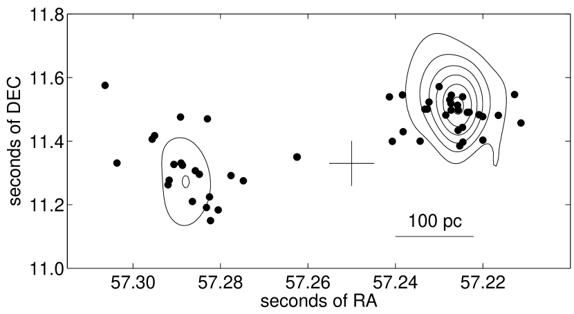
Figure 1: Overall view of the Arp 220 nuclear region. Filled circles are the corrected positions (see Section 2.4 for details) of the 49 compact sources at 18 cm catalogued by Lonsdale et al. (2006). Contours show a 6 cm delay–rate map (“Single baseline snapshot image”) obtained from a 10 minute scan with the Ar–Eb baseline in project EP049. Contours are drawn 500 $\mu$Jy apart starting from 500 $\mu$Jy. The data was tapered in time and frequency using a Chebyshev window to reduce sidelobes, resulting in a delay–rate beam of FWHM $\sim$200 mas and a map noise of $\sim$42 $\mu$Jy. The cross indicates the reference position $\alpha_{2000}=$15^h34^m57.^s25, $\delta_{2000}=+$23^∘30′11.″33

The data were correlated on the EVN correlator at JIVE in the Netherlands. Classic AIPS was used for the calibration stage and fringe fitting resulting in a detection with a signal to noise ratio of $\sim$60. We then used our own software to make a delay–rate map (see Thompson et al. 2001, and references therein) from the Ar–Eb data which showed two sources associated with the eastern and western nuclei with fluxes of 1.0 and 2.9 mJy respectively (see Figure 1). A delay–rate map made from the Ar–Wb data was similar but had larger noise. The significance of these maps is that although they appear to have low resolution they are in fact only sensitive to structures which are compact on the Ar–Eb baseline. Therefore although for Figure 1 the delay–rate beam is large ($\sim$200 mas) the map includes only emission contributed by features which are less then 2 mas in size and so does not include any of the extended emission seen in previous 6 cm MERLIN maps (Rovilos et al. 2003). This image therefore provided the first evidence for the detection of the Arp 220 compact features at 6 cm. Given the large bandwidths now spanned by 1 Gbit s^-1 observations this delay–rate (or ’single baseline snapshot imaging’) technique is a useful method for detecting and imaging at moderate resolution compact emission in starbursts.

2.2 VLBA 13, 6 and 3.6 cm Follow-up

Initially believing that our global 6 cm observations (see Section  2.1) had detected two new bright SNe we applied for and obtained rapid–response VLBA (NRAO) observations. These observations used dual polarization at wavelengths of 13, 6 and 3.6 cm at a total data rate of 256 Mbit s^-1 and were made on 2006 January 9 th (experiment BP129). To optimize $uv$ coverage the allocated 10 hours were split into 8 blocks of $\sim$70 minutes. Each block was equally divided into 23 minutes at each wavelength. The data were reduced using classic AIPS. After manual flagging using SPFLG, instrumental delay and rates were removed by fringe fitting the relatively strong (4 Jy) calibrator J1613+3412 and the solutions applied to the whole experiment. Atmospheric effects were removed by using phase referencing with 2 minute scans on the nearby calibrator J1532+2344 (0.°55 away from Arp 220) alternating with 3.5 minute scans on the target at each wavelength (Wrobel et al. 2000; Beasley & Conway 1995). The observed phases were very stable at all wavelengths. At 3.6 cm typical differences in phase between adjacent calibrator scans had rms values of $\sim$4^∘, and visual estimation of the uncertainties in interpolated phase were at a comparable level. Given the small separation between the target and the calibrator the effect of angular variations on phase errors should be negligible, hence we do not expect any appreciable effect on source amplitudes due to phase incoherence. Amplitude calibration was based on system temperature measurements for each antenna provided as TY tables; based on previous experience with the VLBA we estimate these should be accurate to $\sim$5%.

At each of the three wavelengths the task IMAGR was used to produce 2048$\times$2048 pixel images of both the western and eastern nuclei regions with pixel spacing of 0.25 mas pixel^-1 In order to reduce imaging artifacts from poorly sampled extended emission a minimum $uv$ distance of 10 M$\lambda$ was used at 6 and 3.6 cm. After experimentation the most sensitive image at 13 cm was obtained using a minimum baseline cutoff of 5 M$\lambda$. To maximize image sensitivity pure natural weighting was used at each wavelength. Only a couple of hundred CLEAN components were needed before the residual image became noise-dominated. Despite the use of $uv$ limits the final CLEAN images contained weak ripples of $\sim$20 mas of wavelength possibly introduced by the griding algorithm of IMAGR. In a final step these ripples were removed by taking the Fourier transform of the images, eliminating the associated spikes and inverse-Fourier transforming back to obtain almost ripple free images. The final images at 6 cm and 3.6 cm achieved the theoretical noise but the noise at 13 cm was somewhat larger (see Table 1). This may be due to to the remaining effects of extended structure or possibly the weakness of the calibrator at this wavelength.

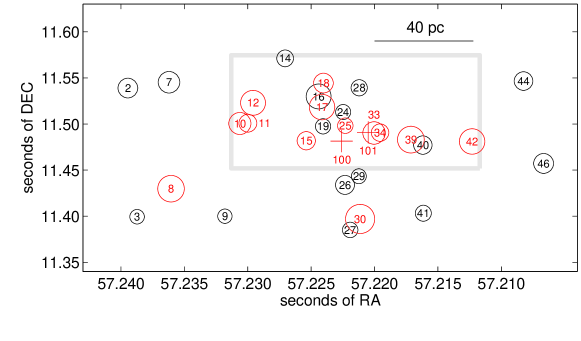
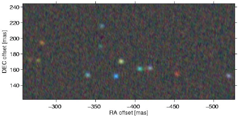
Figure 2: The distribution of compact radio sources in the western nucleus. Top: Detected sources at 18 cm wavelength shown as circles with area proportional to flux density (as reference, source number 30 is 1.23 mJy). The plotted numbers, prefixed by “W” for “West”, are the source names as defined by Lonsdale et al. (2006), including two new sources (W55 and W56). Sources detected at any wavelength shortward of 18 cm are shown in red. Red crosses indicate the positions of two previously uncatalogued sources. The gray rectangle indicates the relative position of the composite image shown in the bottom panel. Bottom: Red, Green and Blue composite image displaying respectively 13, 6 and 3.6 cm images from experiment BP129. The axes of this image are in mas from the reference position indicated by the cross in Figure 1. An expanded contour image of the region around W33 is shown in Figure 4

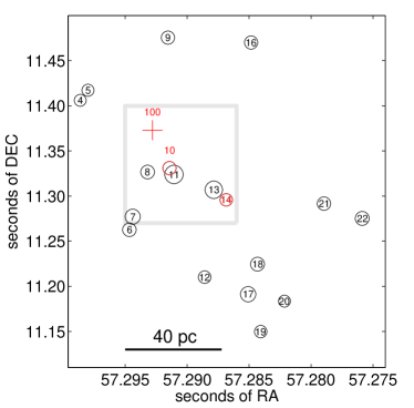
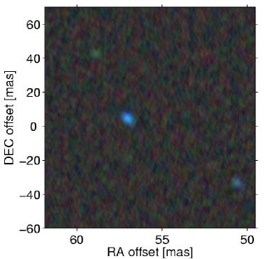
Figure 3: The distribution of compact radio sources in the eastern nucleus. Left: Detected sources at 18 cm wavelength shown as circles with area proportional to flux density. The plotted numbers, prefixed by “E” for “East” are the source names as defined by Lonsdale et al. (2006), including one new source (E24). Sources detected at any wavelength shortward of 18 cm are shown in red. Red crosses indicate the position of the previously uncatalogued source. The gray rectangle indicates the relative position of the composite image shown in the right panel. Right: Red, Green and Blue composite image displaying respectively 13, 6 and 3.6 cm images BP129. The axes of this image are in mas from the reference position indicated by the cross in Figure 1.

Images of the western and eastern nuclei are presented as two RGB composite images (Figures 2 and 3). These images were constructed by assigning to the R, G and B channels versions of the 13, 6 and 3.6 cm images produced by restoring the CLEAN components using a circular beam of 5 mas at all three wavelengths. These images clearly show that the detected sources have very different colors demonstrating their wide variety of spectral properties. In addition to these images an image was made at 3.6 cm wavelength using uniform weighting to check for source resolution. All except one of the sources (see Section 5.2.3) was unresolved.

2.3 Additional Data

In addition to our own BP129 observations we also reduced archival 6 cm VLBA data from 2003 January 2 (BN022) consisting of 2 hours at a data rate 128 Mbit s^-1. These observations used a phase referencing cycle of 3 minutes on Arp 220 and 1 minute on the calibrator J1516+1932. These data were reduced following the procedures described in the previous section. Finally to aid in the search for sources at high frequency and for constraining the long wavelength part of the source spectra we have used data from global 18 cm experiments GD17A (Lonsdale et al. 2006) and GD17B (Thrall et al.in preparation). The latter data was observed approximately one year before BP129, however most 18 cm light curves are known to vary slowly (Rovilos et al. 2005) and so these data can be used to extend the spectra obtained from BP129. A summary of all the available data indicating the achieved sensitivities and resolutions is given in Table 1.

2.4 Source Astrometry and Previous 6 cm Observations

Comparing our 13 cm image from experiment BP129 with published 18 cm images (Smith et al. 1998) we found 4 bright sources with the same relative separations, however the absolute positions of the two images differed by $\sim$100 mas in declination. Careful checking convinced us that the positions from BP129 are correct and that it is the published positions that are wrong. In particular 6 cm source positions from EP049, BP129 and BN022 all agree.

Previously published 18 cm VLBI continuum and spectral line images have all been made by phase-referencing to the brightest 1667 MHz OH maser in the western nucleus (Smith et al. 1998; Rovilos et al. 2003). Absolute positions were then assigned by adding the absolute position of this maser as determined from an old MERLIN astrometric observation. The fact that we find an error in absolute position which is entirely in one coordinate and is very close to 100 mas suggests that a typographical error was made when either originally recording or later manually copying the position of this brightest maser. Note that this astrometric error effects both the published absolute positions of 18 cm continuum sources and OH masers. It will not of course effect the relative positions of masers and compact 18 cm continuum.

A consequence of the above astrometric error is that previous searches for sources at 6 cm were made centered on the wrong field. However this does not appear to be the primary reason why previous observations at 6 cm failed to detect anything. The 6 cm data from Rovilos et al. (2005) has been re-reduced and the correct positions searched but only hints of detections have been found. The reason is most likely the large angular distance (5.°76) to the calibrator combined with the fact that these observations were made near solar maximum when ionospheric effects could have been significant even at 6 cm. In contrast, the new absolute positions derived from our BP129 VLBA observations are accurate to within a few mas (Pradel et al. 2005). It should be noted that the nearby calibrator used for these observations was not catalogued at the time of the earlier imaging attempts at 6 cm (Petrov et al. 2005).

3 RESULTS AND ANALYSIS

3.1 Source Detection Criteria

Visual inspection of Figures 2 and 3 shows that many sources are clearly detected at short wavelengths. However to more rigorously define a complete list of detections we defined quantitative detection criteria. We made two passes through the BP129 images, first searching around the positions of catalogued 18 cm sources and then searching the whole area of the eastern and western nuclei. In the first pass sources could be accepted as real at a lower signal to noise ratio than in the second pass because of the much smaller number of beam areas searched. In the first pass we searched separately at each of our three wavelengths; a source was considered a detection if it was detected at one or more wavelengths. Since sources missed in the first pass would be uncatalogued at 18 cm (and hence very weak at both 18 and 13 cm) these sources would have spectra that peak at high frequency. Therefore in the second pass we only searched a single composite image formed by averaging our 6 and 3.6 cm images.

In the first pass we conservatively took the 18 cm beam size as our search area around each of the 49 known positions. The number of independent beam areas searched at each wavelength ($\lambda$) was then $N_{s}=49(18/\lambda)^{2}$. Analysis of the histogram of the images in regions away from detected sources showed distributions that were very close to Gaussian allowing the use of Gaussian statistics. Setting the detection criterion as any spike within a given search area above $\eta\sigma$ the probability that one or more entries in the list of detected sources is a noise spike is $F=1-P(I<\eta\sigma)^{N_{s}}$, where $P(I<\eta\sigma)$ is the cumulative probability of a noise spike at a given beam area being less than $\eta\sigma$. At each wavelength we chose $\eta$ such that $F$ was 0.5%. The resulting detection limits at 13, 6 and 3.6 cm are 3.8, 4.1 and 4.4$\sigma$ respectively. Using these criteria a total of 15 sources were detected in the first pass.

In our second pass we then looked for new sources at any other position contained within two square fields of 512$\times$512 mas enclosing the eastern and western nuclei (see Section 2.2). As explained above we searched a composite image made by averaging the 6 cm and 3.6 cm images. This time the area searched was much larger than in the first pass, therefore for a 0.5% confidence of false detection the required detection limit was $5.1\sigma$. In this second pass we detected 3 new sources (2 in the west). In total, despite our rather modest sensitivity, we detected a total of 18 sources (see Table 2). Given that in the first pass three separate searches were made (one at each wavelength) and one search done in the second pass, all with 0.5% confidence of false detection, we estimate an overall 2% probability that one or more of the sources in Table 2 is a false detection.

It should be mentioned that the BP129 image at 3.6 cm shows several point like features that lie just below our detection threshold and are mostly located in the region with the highest density of sources (within 20 mas of position ($-$380, 160) mas in the bottom panel of Figure 2). Almost certainly some of these features will be confirmed as detections in higher sensitivity observations.

3.2 Source Structure

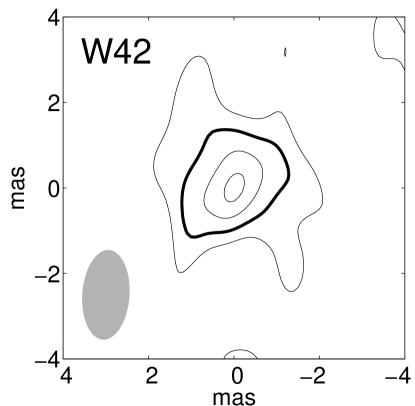
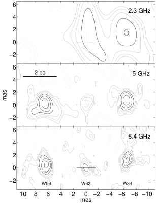
Figure 4: Detailed structure of source W42 and of the W33 region. Left: Contour map of W42 produced from the 3.6 cm wavelength uniformly weighted image. Contour levels are $-$25, 25, 50, 75 and 95% of the peak (see table 2). The 50% contour is drawn with a thick line and the $-$25% ones with dashed (none visible). The 50% contour appears elongated in the NE–SW direction with respect to the beam (shown in the bottom left corner) indicating source resolution. Right: Contour maps of the W33 region at 13, 6 and 3.6 cm. Contour levels are $\ldots,-2,-\sqrt{2},\sqrt{2},2\ldots$ multiplied by the corresponding map noise (see Table 1). Contour levels below the detection threshold at every frequency are drawn in gray. Negative contours are drawn with dotted lines. The axes are in mas relative to the peak in the 3.6 cm map whose position is indicated by a cross in all three panels (see Table 2)

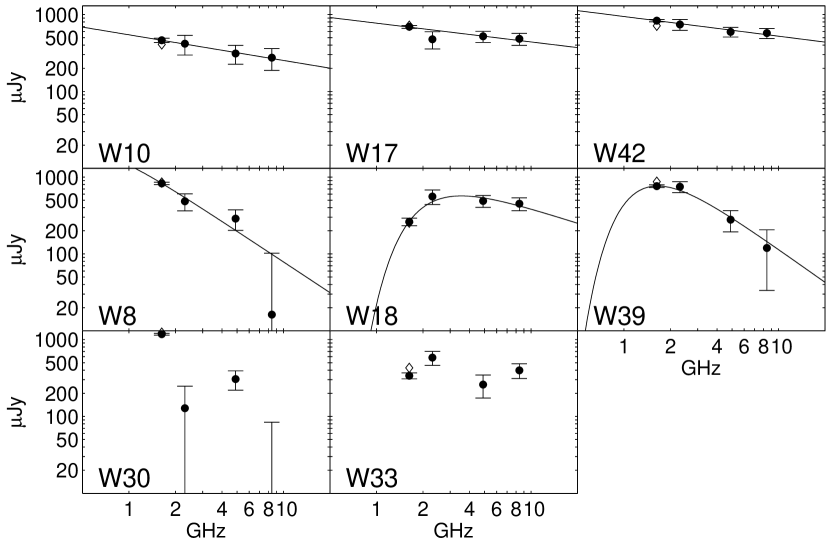
Figure 6: Spectra and models for the short wavelength sources detected in the original 18 cm sample of Smith et al. (1998) (class L sources, see Section 3.3). In all cases error bars are plotted at $\pm 1\sigma$ about the measured value given in Table 2. When the measured flux density is negative only the upper error bar is plotted. The first row shows three sources with relatively flat spectra. The middle row shows the remaining sources that are well fitted by a power law synchrotron plus FFA model (see Section 4.1). Finally the last row shows two sources for which good fits could not be obtained. The data at 13 cm (2.3 GHz), 6 cm (5 GHz), 3.6 cm (8.4 GHz) were taken from simultaneous observations in BP129. The 18 cm data from earlier epochs GD17A and GD17B are shown as filled circles and open diamonds respectively (in some cases these data points overlie each other). Error bars are shown at $\pm\sigma$ (see Table 1) The curves shown are the best fits of the synchrotron plus FFA model spectrum described in section 4.1 as fitted to the data at all four wavelengths. For sources W30 and W33 no reasonable fits could be obtained and therefore no model is plotted.

The only resolved source at 3.6 cm is W42. This source is located $\sim$100 mas to the west of the region with the highest surface density of sources (see Figure 2). Along the position angle corresponding to the beam minor axis the FWHM of W42 is about twice as big as the beam FWHM (see Figure 4-Left). The fact that other sources were unresolved shows that the resolution of W42 is not an artifact of residual phase errors in the data. Another source deserving special attention is W33 which in addition to its peculiar spectrum (see Figure 6) shows possible signs of an elongated structure in the North–South direction at 13 cm (see Figure 4-Right). This source is tightly located between two bright sources (W56 and W34) and lies near the edge of a patch of diffuse 18 cm emission covering the central region of the western nucleus (Thrall et al. in preparation). We speculate about the nature of this source in Section 5.2.4

3.3 Source Variability

In order to search for correlations between source spectral properties and source age we classify our detected sources in terms of their broad 18 cm variability properties. A more detailed variability study including detailed light curve modelling will be presented in a subsequent paper (Thrall et al. in preparation). We define four classes of sources:

Class L (Long lived) These are 8 sources already detected by Smith et al. (1998) based on observations in 1994, hence these sources are at least 11 years old. In addition analysis of the first 6 years of monitoring data by Rovilos et al. (2005) showed that all these sources had slow or undetectable decays of their 18 cm flux densities and are therefore likely to be significantly older.

Class R (Rising) These are 4 sources not detected by Rovilos et al. (2005) but which are detected in the latest 18 cm epochs at flux levels significantly above the Rovilos et al. (2005) detection limits. W11, W25 and W34 were present in GD17A but not in the 18 cm experiment (GL26B) made 12 months earlier (Lonsdale et al. 2006). Source W11 was present in both GD17A and GL26B but not at earlier epochs (Lonsdale et al. 2006).

Class S (Single epoch) These are 3 sources only detected in our new high frequency data and not in any 18 cm epoch.

Class A (Ambiguous) These are sources with ambiguous variability classification. For instance one of the three sources in this class (W15) is detected in both GD17A and GD17B at similar flux densities, but at levels below the Rovilos et al. (2005) detection limits, therefore it could be either a new source or a long lived stable source not detected earlier because of sensitivity limitations. Similar considerations apply to source E14. Source E10 was not detected by Rovilos et al. (2005), was detected in GD17A, but not detected in GD17B.

In addition to the above classification scheme, it is also interesting to consider possible variations in 6 cm flux densities by comparing our data with the BN022 data taken just over 2 years earlier. Considering the thermal noise on both epochs only two sources show $>2\sigma$ variations, namely W18 ($-$625 $\mu$Jy) and W33 ($-$505 $\mu$Jy). Surprisingly both are class L sources. W33 has other unusual properties in addition to its variability and is discussed further in Section 5.2.4.

3.4 Source Spectra

To determine the spectra of our detected sources we first defined a source position based on the highest frequency detection, then at this pixel we determined the brightness at each of the three simultaneously observed wavelengths (13, 6 and 3.6 cm). Tests fitting gaussians to the four brightest sources at 3.6, 6 and 13 cm showed consistent positions at the three wavelengths to within $\sim$0.5 pixels in each coordinate (one pixel being 0.25 mas). Since the source position is defined at 3.6 cm, the maximum impact of any registration offset on the derived spectra is set by it effect at 6 cm. At this wavelength the map registration uncertainty amounts to less than 10% of the beam minor axis FWHM and will contribute only a 2% error on the amplitude which is negligble relative to the map noise. The resulting source flux densities using the above procedure are given in Table 2. In some cases the reported numbers are less than the noise or are negative, but these measurements are still useful for constraining spectral fits (see Section 4.2). An exception to the above procedure is the resolved source W42 (see Section 5.2.3) for which the integrated flux density at 3.6 cm was determined within a box containing the source.

For the 18 cm flux densities a slightly different procedure was followed because these data were not taken simultaneously with the rest of the wavelengths and so exact position registration at the pixel level could not be assured. For GD17A fluxes are taken from Lonsdale et al. (2006) in the case of tabulated detections, otherwise the map was searched at the detected high frequency position within the 18 cm beam area for anything above $3\sigma$. In no cases was any new detection found, these sources are reported in Table 2 as $3\sigma$ upper limits. For GD17B the largest peak within an 18 cm beam area of the high frequency position was located, in most cases large SNR detections were found. In cases with no peak above $3\sigma$ these upper limits are reported in Table 2.

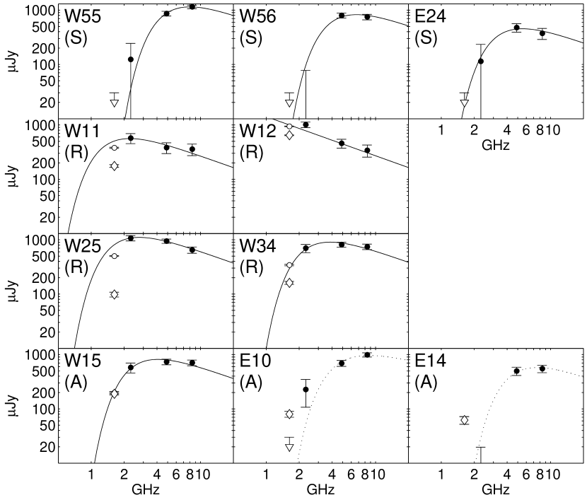
Figure 5: Spectra and models of short wavelength detected sources not in the original 18 cm sample of Smith et al. (1998); these sources are either new since 1995, weak at long wavelengths or both. The variability subclass to which each source belongs (R, S and A, see Section 3.3 for definition) is indicated in the top left corner of each spectrum. The data at 13 cm (2.3 GHz), 6 cm (5 GHz), 3.6 cm (8.4 GHz) were taken from simultaneous observations in BP129 and are shown as filled circles. For those points error bars are plotted at $\pm 1\sigma$ about the measured value given in Table 2. In cases where the measurement gives a negative flux density only the upper error bar is plotted. The 18 cm data comes from the earlier epochs of GD17A and GD17B, shown as diamonds and open circles respectively. In the case of detections at this wavelength error bars are plotted at $\pm\sigma$. If a source is undetected at one or more of the 18 cm epochs an upper limit is plotted. The curves shown are the best fits of the model spectrum described in section 4.1 obtained by fitting only to the simultaneous 13, 6 and 3.6 cm data from the BP129 epoch. For sources E10 and E14 the best fits are shown with dotted lines indicating that these models were unable to fit all the data within the error bars.

All the measured spectra for sources in classes R, S and A are displayed graphically in Figure 5. Sources in class L are displayed in Figure 6. Taken together a wide variety of spectral shapes are seen from inverted to flat to steep. Overall the distribution of spectra are very similar to those of the compact sources detected in knot A of the starburst Arp 299 (see Neff et al. 2004). Further discussion and modelling of our observed Arp 220 spectra is presented in § 4.

3.5 Source Spatial Distribution

An initial impression from Figure 2 is that the 15 short wavelength detections in the western nucleus (red circles in the top panel) have approximately the same spatial distribution as the 18 cm sources from Lonsdale et al. (2006). However if we only consider sources not seen in Smith et al. (1998) (i.e. classes R, S and A) which have rising or peaked spectra (see Figure 5), these appear to be more centrally concentrated. All seven such sources are found within the gray rectangle in Figure 2. In contrast amongst the 18 cm sources of Lonsdale et al. (2006) the fraction inside the rectangle is only $17/29=0.58$. If the class R, S and A sources have the same spatial distribution there is only a 2.4% probability of all being within the rectangle. However this is only an a posteriori statistic and so must be treated with caution. Future observations plus robust statistical tests are needed to check it. Note even if true it does not necessarily imply a difference in spectral properties with position. These results might be explained by differences in overall luminosity combined with the present high flux detection threshold at short wavelength. Supporting this explanation is the fact that the median 18 cm luminosity is a factor of two larger inside the rectangle than outside. Furthermore a Kolmogorov-Smirnov test finds only a 6% probability that the 18 cm sources inside and outside are drawn from the same flux density distribution.

4 ANALYSIS OF SOURCE SPECTRA

4.1 Cause of Low Frequency Spectral Turnovers

The majority of the spectra shown in Figure 5 are consistent with power law synchrotron spectra with turnovers below some critical frequency. Such spectra are typically observed in both SNe and SNRs (Weiler et al. 2002; Allen & Kronberg 1998). In principle the low frequency turnovers could be due to either synchrotron self absorption (SSA) or FFA. Although the former has been successfully invoked for weak Type II and Type Ib/c SNe (Soderberg et al. 2005) in all successfully modelled powerful Type II SNe and SNRs FFA is the dominant process (Weiler et al. 2002). This is confirmed by the fact that for those powerful SNe and SNRs sources which are resolved the brightness temperatures are too small for SSA to operate.

For SSA to occur at a given frequency a characteristic relationship between source luminosity and diameter is required (Chevalier 1998). For a given shell expansion speed this implies a relationship between peak luminosity and rise time. Inversely for an observed combination of these parameters there is an associated expansion speed required for SSA to dominate (see Figure 4 in Chevalier 1998).

Sources of class R have spectra peaking around 4 GHz and peak luminosities of $\sim$$10^{28}$ erg s^-1 Hz^-1. If a rise time at 4 GHz of over 2 years is assumed (the time between GD17A detections and BP129) then these sources lie in the region of the luminosity–rise time diagram occupied by Type IIn SNe. In turn, for SSA to apply in these sources, the required expansion velocities are $<3000$ km s^-1 which is considered too slow for this kind of SN (Chevalier 1998). The longer lived class L sources with spectral turnovers would require even slower expansion velocities and so are even more unlikely to be affected by SSA. We have no idea of the age or rise times of class S sources. In principle these could be rare luminous Type Ib/c sources with fast rise times and hence could be affected by SSA. However it seems improbable that we detect 4 such sources given the short time their luminosities peak. More likely these are class R sources observed at an earlier evolutionary stage. We conclude that SSA is unlikely to be a significant cause of the low frequency cutoff in any of our sources. We will be able to test this assumption using future observations over a wide frequency range by examining the shape of the low frequency cutoff; unfortunately the present sparse non-simultaneous spectral data does not allow such a test.

4.2 Free-free Absorption Model

In this section we fit the observed spectra as a generic power law plus FFA. We leave to section 5.1 the question of whether the data are more consistent with SNe or SNRs. In SNe the FFA occurs mostly in the wind blown bubble from the progenitor star. In contrast in SNRs the FFA is due entirely to the foreground ionized ISM. The model spectra we fitted are described by

$$S_{\nu}=S_{\rm sy}(\nu/1.63)^{\alpha}\exp\{{-\tau_{18}(\nu/1.63)^{-2.1}\}}$$ (1)

where $\nu$ is the frequency in GHz, $S_{\rm sy}$ is the 18 cm unobscured synchrotron flux in $\mu$Jy, $\alpha$ is the optically thin non-thermal spectral index and $\tau_{18}$ is the optical depth at 18 cm. This model corresponds to all the FFA being foreground to the synchrotron emission and all parts of the source being subject to the same foreground opacity. Note the latter is not true if the FFA absorbing medium is clumpy with clump scale sizes smaller than the emitting source in which case more complex models will apply (Natta & Panagia 1984, Conway et al., in preparation).

The fitting proceeded by finding for each source the global minimum of the $\chi^{2}$ metric in a gridded three dimensional volume. To improve accuracy after an initial coarse search a second search was done using a denser grid around the coarse solution. We note that for some sources at some wavelengths the measured flux densities were negative. However, these values are formally our best estimates and therefore were considered in the fitting procedure. This is a simpler and less potentially biased procedure than fitting a mixture of measurements and upper limits.

For the class L sources we fitted all three free parameters of the model to the four spectral data points provided by the three wavelengths in BP129 plus 18 cm data from the non-simultaneous GD17B observations (taken 0.84 year before). The use of the non simultaneous 18 cm data in the spectral fitting is justified for the class L sources because they are known to have low variability at this wavelength (Rovilos et al. 2005). Furthermore in all cases the GD17A and GD17B measurements are consistent within the error bars confirming low recent variability (compare diamonds and circles at 18 cm in Figure 6).

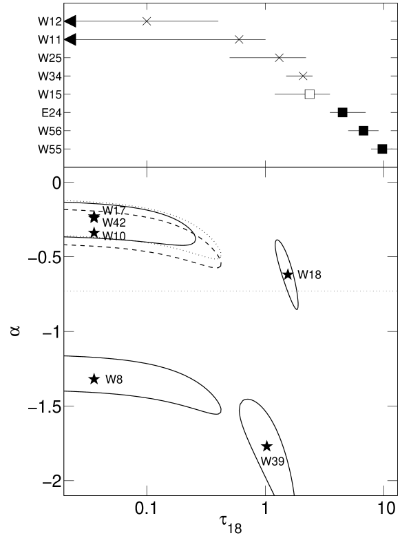
Figure 7: Summary of spectral model fitting results for the power law plus free-free absorption model presented in Section 4.2. Bottom: The stars indicate the best fit values of $\tau_{18}$ and $\alpha$ for the six class L sources with three parameters fits to four wavelength spectral data. Note that for sources W8, W10, W17 and W42 the optimum value of $\tau_{18}$ is estimated as zero which cannot be plotted on a on a logarithmic scale and therefore these points are plotted at an arbitrary small value of $\tau_{18}$. The surrounding contour around each plotted point delineates the region in which the reduced $\chi^{2}$ increases by less than one compared to the best fit, indicating the 68% confidence region. (The contours for W17 and W10 are drawn in dotted and dashed line respectively). The dotted horizontal line is plotted at the value of spectral index assumed for the two parameter fits shown in the top panel. Top: Shows fitted $\tau_{18}$ for those sources fitted using only the three wavelengths from BP129 and fixing synchrotron spectral index $\alpha=-0.72$ (see section 4.2 for details). Lines indicate $1\sigma$ error bars. Sources from variability classes S, R, and A are indicated as filled squares, crosses, and empty squares respectively.

Solutions fitting the data within the error bars (reduced $\chi^{2}<1.5$) were obtained for 6 of the 8 class L sources, the exceptions being W30 and W33. The optimum values for $S_{\rm sy}$, $\alpha$ and $\tau_{18}$ are summarized in Table 2 and the corresponding model spectra are overlayed on the data in Figure 6. Note that in some cases the best solution had a slightly negative opacity $\tau_{18}\approx-0.1$ which is clearly unphysical. In those cases we set $\tau_{18}=0$ and found the values for the other parameters which minimized $\chi^{2}$; in all such cases the final $\chi^{2}$ was only slightly increased (by $\lesssim 0.5$). In addition to finding the optimum values, the region of $\tau_{18}$ and $\alpha$ around the best fit was searched finding for each combination the optimum $S_{\rm sy}$ and recording $\chi^{2}$. The area over which this $\chi^{2}$ increased by less than one compared to the global minimum was used to define a 68% confidence ellipse around the $\tau_{18}$ and $\alpha$ solution. These confidence ellipses are plotted in the bottom panel of Figure 7 and show in most cases a significant correlation between the solutions for the two parameters.

For the class S, R, and A sources long term monitoring data at 18 cm is not available and we cannot assume that the GD17B data approximates the 18 cm flux density at the time of the BP129 observations. In fact in many cases comparison of GD17A and GD17B data suggests significant variability. Fitting a more complex time variable model adds more unknowns and we defer such an attempt to a later paper when we have more data. Instead here we choose to fix $\alpha$ at a value of $-0.72$, corresponding to the median synchrotron spectral index of the 9 well studied Type II SNe from Weiler et al. (2002) and then fit the remaining parameters $\tau_{18}$ and $S_{\rm sy}$ to the three simultaneous frequency data points from BP129. We chose to do this because fitting the full three parameter model to only three data points resulted in large uncertainities and in some cases unphysical optimum solutions which were clearly dominated by noise. Note that the above fitting method can only hope to show consistency with the assumed spectral index $\alpha$ but does not prove it.

Using the above procedure good fits passing through the three simultaneous frequencies and consistent with a reasonable evolution of the 18 cm flux densities are obtained for 8 of the 10 sources (see Figure 5). The exceptions are E14 and E10. The fit for E14 passes through the fitted data points but predicts an 18 cm flux density very different from the consistent values seen in GD17A and GD17B. In E10 the fit is a little too steep to fit the 13 cm data point, on the other hand such a fit is consistent with the apparently rapidly falling 18 cm flux density which may point to a problem with the 13 cm data point. For the 8 well fitted sources the optimum values of $\tau_{18}$ obtained are shown in the top panel of Figure 7 including 1$\sigma$ error bars.

4.3 Fitted Spectral Indices and Opacities

Figure 7 plots the fitted $\alpha$ versus $\tau_{18}$ using different symbols for the different variability classes defined in Section 3.3. This figure shows that the highest opacities $\tau_{18}>4$ all occur in class S sources, which are those that are newly detected. There is only one class A source giving a good fit and this also has quite a large $\tau_{18}=2.4$. Of the class R or rising sources 3 out of 4 have $0.7<\tau_{18}<2.1$. Finally amongst the long lived class L sources 4 out of 6 have spectra consistent with zero opacity, There appears therefore to be a rough correlation of decreasing opacity with source type from S to R to L. Although the exact value of $\tau_{18}$ is model dependant and Figure 7 combines sources with 2 and 3 parameter fits, the results help quantify the visual impression given from the data in Figures 5 and  6 of decreasing turnover frequency along the above sequence. In section 5 we discuss this turnover/opacity correlation in terms of decreasing opacity with source age, consistent with a source evolution from young SNe to more evolved SNRs.

For the class L sources there was enough data to allow us to fit for $\alpha$ (see Section 4.2). This fitting gives three sources with flat spectra ($\alpha>-0.5$), one with intermediate spectral index ($\alpha\approx 0.6$) and finally two with steep spectra ($\alpha<-1$). Another source falling in this last category is W7 which is not listed in Table 2 because it was not detected at any of the BP129 wavelengths; this non detection however implies it has a very steep spectrum ($\alpha<-1.5$).

5 DISCUSSION

5.1 Supernovae or Supernova Remnants?

An important question is whether the compact radio sources in Arp 220 are primarily SNe (interacting with their progenitor’s CSM) or SNRs (interacting with the denser ISM). Here we discuss the radio properties expected from these two cases and compare with past and present observations.

5.1.1 Background

Despite the extreme environment in the nuclei of Arp 220 and other ULIRGs it is expected that wind blown bubbles with a density profile $\rho_{w}(r)=\rho_{o}r^{-2}$ will still form around progenitor stars (Chevalier & Fransson 2001, Arthur, astro-ph/0605533). Hence there should remain a distinction between the SN phase, when the blast-wave transits this declining density wind, and the SNR phase in a constant density ISM. Equating the ram pressure of the wind with the external ISM pressure the expected bubble radius is

$$r_{b}=0.2\dot{m}_{-4}^{0.5}v_{w1}^{0.5}p_{7}^{-0.5}\rm\quad pc$$ (2)

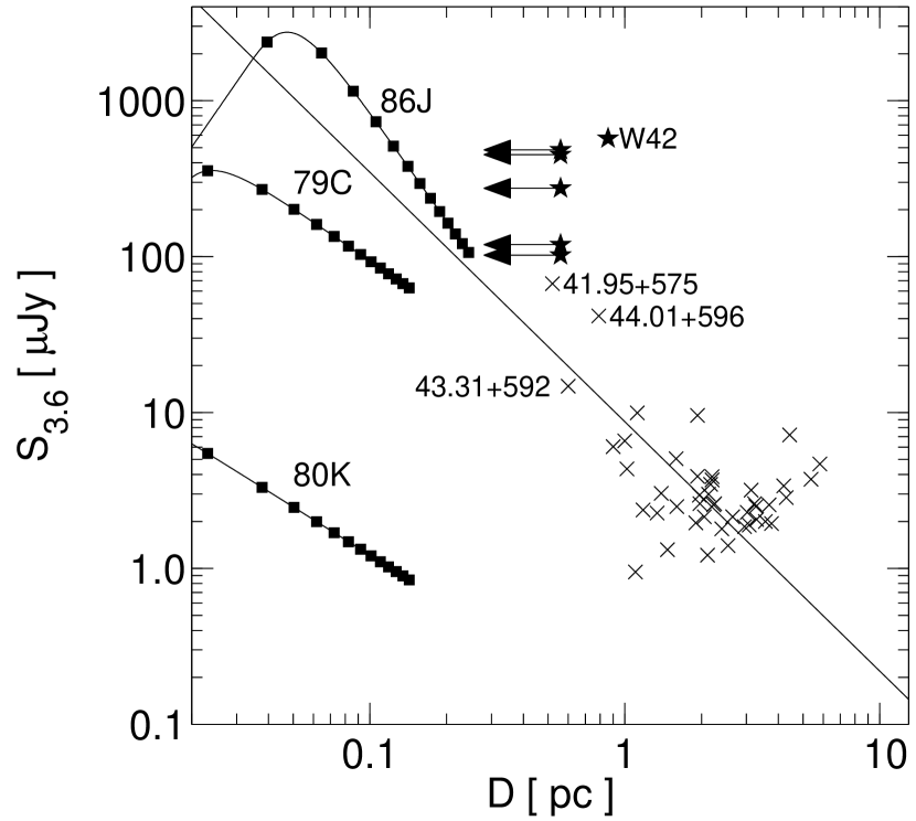
Figure 8: Illustration of the expected 3.6 cm flux density and sizes of observed SNe and SNRs if placed at the distance of Arp 220. The SN tracks for SN1986J (Type IIn), SN1979C (Type IIL) and SN1980K (Type IIL) were produced using the light curve fits given in Weiler et al. (2002) combined with the deceleration parameter from Bietenholz et al. (2002) for SN1986J and assuming free expansion at $10^{4}$ km s^-1 for both SN1980K and 1979C. The square markers along each track indicate time evolution and are 1 year apart. Crosses indicate the location of 45 SNRs in M82 from Huang et al. (1994) with their fluxes scaled down to the distance of Arp 220. The diagonal line is derived from the empirical relation between SNR surface brightness and diameter ($\Sigma-D$) fitted by Huang et al. (1994) converted to flux density at the distance of Arp 220. Stars show data for seven class L sources (W33 is not shown). Horizontal arrows indicate upper limits in size for the unresolved sources.

where $\dot{m}_{-4}$ is the mass loss rate in units of $10^{-4}$ $\rm M_{\odot}$ year^-1, $v_{w1}$ the wind speed in units of 10 km s^-1 and $p_{7}$ the interstellar pressure in units of $10^{7}$ K cm^-3. During the initial SN phase, the shock-wave moves through the stellar wind and the optically thin radio luminosity of the synchrotron emitting shell at a fixed radius is proportional to $\rho_{o}^{k}$ or $(\mbox{$\dot{m}_{-4}$}/v_{w1})^{k}$ where $k$ is in the range 1.4 to 2 (Chevalier et al. 2006). It follows that there is a very wide range in radio luminosity for SNe depending on the wind properties (see Figure 8). The most luminous RSNe with the densest winds are optically classified as Type IIn followed by luminous Type IIL/b classes (for a recent review of SN types and their radio emission see Chevalier 2006). Such luminous objects are thought to be quite rare within galactic disks. For instance, Cappellaro et al. (1997) estimate that only 2% of core-collapse SNe are of the Type IIn subclass. However there are significant uncertainties on the fraction of SN types (Chevalier 2005) and these fractions may be strongly dependent on the number of close binaries (Nomoto et al. 1996) which could be radically different in dense ULIRG nuclei.

During the SN phase the radio light-curves are defined by competition between decaying synchrotron emission and decreasing FFA, giving rise to light curve peaks which occur progressively later at longer wavelengths (Weiler et al. 2002).

Sources are expected to enter the SNR phase, and in most cases start to brighten, when the blast-wave reaches the edge of the bubble given by equation 2. The evolution just after this will be complicated as the blast-wave transits shocked wind and possibly (partially) collapsed HII region gas (van Marle et al. 2004; Chevalier et al. 2004). Nevertheless it is expected that radio emission will peak (Cowsik & Sarkar 1984; Huang et al. 1994) at the beginning of the Sedov phase (i.e. when the swept up mass, dominated by the dense surrounding ISM gas, equals the ejecta mass) which occurs at radius

$$r_{s}\simeq 4.1\mbox{$\times$}(M_{\rm ej1}/\mbox{$n_{\rm ISM}$})^{1/3}\rm\quad pc$$ (3)

where $M_{\rm ej1}$ is the ejecta mass in units of 10 $\rm M_{\odot}$ and $n_{\rm ISM}$ is the ISM number density in cm^-3. For $n_{\rm ISM}$$=$$10^{4}$ and $M_{\rm ej1}=0.5$ the predicted size is $r_{s}=0.15$ pc. Once the Sedov phase is reached the radio luminosity is expected to gradually decrease in a way consistent with the Surface brightness–Diameter ($\Sigma-D$) relation for SNR (Huang et al. 1994) . Substituting $r_{s}$ into this relation we obtain a rough estimate of the peak 3.6 cm SNR luminosity of a young SNR of

$$L_{3.6}\approx 2.6\mbox{$\times$}\hbox{$10^{24}$}(M_{\rm ej1}/\mbox{$n_{\rm ISM}$})^{-0.53}\rm\quad erg~{}\hbox{s${}^{-1}$}\hbox{Hz${}^{-1}$}$$ (4)

Eventually when the internal SN gas cools to below $10^{6}$ K energy losses to atomic lines become significant (Draine & Woods 1991) and the radio luminosity decays more rapidly than in the Sedov phase. If the external density is very large ($n_{\rm ISM}$$>$10⁵ cm^-3) then a source can become radiative before it enters the Sedov phase (Wheeler et al. 1980) in which case it will never reach the $\Sigma-D$ relation.

In the model of Huang et al. (1994) the SNRs all lie close to the same $\Sigma-D$ (or Luminosity$-D$) relation because they all release approximately the same kinetic energy ($10^{51}$ ergs) and a constant fraction of this energy is injected into relativistic particles. The more detailed modeling of Berezhko & Völk (2004) confirms that in the early Sedov phase, for a given diameter $D$, the radio luminosity depends only on the SN energy and is independent of the external density. We therefore expect that all core collapse SNe would evolve eventually to join the SNR Luminosity$-D$ relation at some diameter defined by equation 3. Hence for an object like SN1980K (see Figure 8) we can expect a dramatic brightening when the blast-wave encounters the high density ISM and it enters the SNR phase.

An interesting possibility is that the observed new 18 cm radio sources in Arp 220 (Rovilos et al. 2005; Lonsdale et al. 2006) could be such SN/SNR transition objects rather than SNe. Radio luminosity would start increasing when the blast-wave reached the edge of the wind blown bubble and would peak when the swept up ISM gas mass equalled that of the ejecta, hence characteristic rise times would be of order $(r_{s}-r_{b})/v_{\rm ejecta}$. For $v_{\rm ejecta}$=$10^{4}$ km s^-1 a high external density of $n_{\rm ISM}$$=$$10^{5}$ cm^-3 and a pressure of $p_{7}=1$ the rise time would take $\sim$7 years, only somewhat longer than SNe rise times at 18 cm. However since for an emerging SNR the reason for the luminosity increase is quite different than for a SN (a general increase of high energy particles and field rather than reduced FFA) such objects are expected to show very different multi-wavelength light curves. According to the model of Berezhko & Völk (2004) the radio spectrum is expected to keep approximately the same shape during the rise phase and hence we would expect the multi-wavelength light-curves to show similar behavior, in contrast to the characteristic delay between wavelengths observed in SNe.

At the other end of the SN luminosity range (see Figure 8) for objects like SN1986J and SN1979C the observational data are consistent with a fairly smooth luminosity transition between the SN and SNR phases. This might be expected because the progenitors of such powerful RSNe have the densest winds and therefore the smallest density contrasts between their terminating wind and the external medium.

5.1.2 Previous Observations

In their discovery paper Smith et al. (1998) proposed a SN based model for the compact sources in Arp 220 in which all were due to extremely luminous Type IIn SNe. The number of observed sources and the total FIR luminosity were found to be consistent if all these SNe were as radio luminous as the Type IIn supernova SN1986J. Chevalier & Fransson (2001) argued that this model was unlikely because such luminous objects comprise only a small fraction of core-collapse SNe. Observational doubts on the Smith et al. (1998) model were cast by the 18 cm light curve monitoring of Rovilos et al. (2005) which did not show the decay in flux expected from SN1986J like sources. Consequently both Rovilos et al. (2005) and Lonsdale et al. (2006) have suggested that most sources in Arp 220 are instead higher luminosity versions of the SNRs in M82.

The above SNR hypothesis seems plausible if we consider the expected and observed flux densities. In equation 4 we estimated the maximum luminosity of a SNR at wavelength 3.6 cm as a function of ISM density. Assuming a spectral index of $-0.7$ and scaling to the distance to Arp 220 this predicts 18 cm flux densities of $1.2\mbox{$\times$}(M_{\rm ej1}/\mbox{$n_{\rm ISM}$})^{-0.53}$ $\mu$Jy. For the median 18 cm source flux density in the western nucleus of 207 $\mu$Jy (Lonsdale et al. 2006) and assuming $M_{\rm ej1}=0.5$ we obtain an estimated ISM density of $n_{\rm ISM}$=8300 cm^-3 which is consistent with the mean molecular density of 1.5$\times$$10^{4}$ cm^-3 estimated by Scoville et al. (1997).

In addition to the slow evolution of the brightest sources Rovilos et al. (2005) and Lonsdale et al. (2006) also detected some new weak 18 cm sources. These papers propose that these new sources are SNe, implying a mixed SNe and SNRs population. Supporting the SN interpretation for the new sources it was found that if their rate of appearance was taken as the SN rate $\nu_{\rm SN}$ and a standard IMF assumed then the predicted SFR was consistent with that estimated from the FIR luminosity (Lonsdale et al. 2006). A possible difficulty however is the assumption that all core-collapse SNe give rise to RSNe luminous enough to be detected. As described in Section 5.1.1 such luminous radio sources are thought to be rare. One possible explanation is that the new radio sources are instead SN/SNR transition objects (see Section 5.1.1). This and other possible explanations for reconciling the rate of new radio sources and the SFR are discussed further in Section 5.4.

5.1.3 Comparison of New Data and SNe Models

The standard model for the radio emission from powerful RSNe comprises power law emission from a synchrotron emitting shell observed through FFA gas from the ionized CSM (Weiler et al. 2002). This absorption decreases rapidly with time as the blast-wave moves outward. In Section 4.2 we fitted our observed source spectra around the epoch BP129 with such a power law plus FFA model and the estimated spectral indices and opacities were plotted in Figure 7. This plot shows the expected correlation between source age and opacity predicted by the RSN standard model. All the recently detected (class S and R) sources have high opacity, in contrast to those known to be old (class L) which have lower opacity. This strongly suggests a SN origin for the class S and R sources.

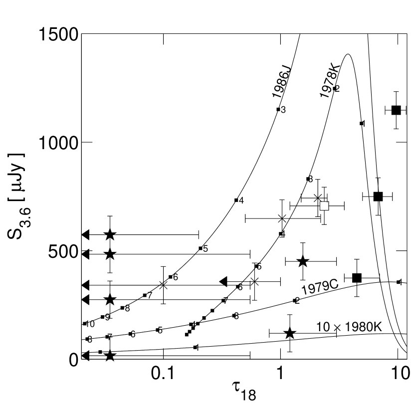
Figure 9: Comparison of observed flux density at 3.6 cm ($S_{3.6}$) and fitted opacity properties ($\tau_{18}$) of the Arp 220 sources to those of well studied RSNe. Arp 220 sources are shown using the same markers as in Figure 7. Lines are the loci traced by the best light curve fit (Weiler et al. 2002) to the observations of SN1986J, SN1978K (both Type IIn), SN1979C and SN1980K (both Type IIL). Note that the curve for SN1980K has been amplified by a factor of 10 for better visualization. Markers on the tracks are labeled with the time after shock break-out in years.

To further check whether the standard SN model applies to our sources Figure 9 plots the fitted $\tau_{18}$ versus flux density at 3.6 cm wavelength ($S_{3.6}$). Superimposed are loci traced by fitted models to four powerful Type II SNe with well sampled multi-frequency light curves (Weiler et al. 2002) scaled to the distance of Arp 220. $S_{3.6}$ and $\tau_{18}$ are natural coordinates to plot our data, since for sources beyond the 3.6 cm peak luminosity they decouple the intrinsic strength of the synchrotron emitting shell from the foreground absorption. In this diagram the effect of small foreground ISM opacities, which are insufficient to affect the 3.6 cm flux densities, is to move the SN tracks to the right by adding a constant $\tau_{\rm ISM}$.

Figure 9 shows that for all the well fitted sources in classes S, R and A both the opacities and luminosities are in the range defined between the most luminous detected Type IIL source SN1979C and the Type IIn source SN1986J. The best fit is in fact to the intermediate luminosity Type IIn SN1978K. However, if there is a foreground ISM opacity at 18 cm of $\tau_{18}\approx 1$ then SN1986J instead provides the best fit. In both cases the required ages as of the BP129 observational epoch (January 2006) would be in the range 1 to 7 years. This result suggests that sources in these three variability classes are powerful SNe.

In contrast it seems very difficult to explain class L sources using the standard RSN model. Three of them (W10, W17 and W42; the three relatively flat spectrum sources shown on the top row of Figure 6) have $\tau_{18}<0.3$ and 3.6 cm fluxes over 250 $\mu$Jy. These could be consistent with objects like SN1986J but only if they had ages $<8$ years, but this is less than their minimum ages ($>11$ years) ruling out a standard SN origin. Sources W18 and W39 could be SNe, however both sources have steep spectra (see middle row of Figure 6) and the weakness of their 3.6 cm flux could be ascribed to this. Finally source W8 is in a part of the diagram that could be reached by SN models but again the required age is much smaller than is observed.

5.1.4 Comparison of New Data With SNR Models

In the previous section it was shown that class S, R an A sources are consistent with being RSNe. In contrast for the older class L sources known since Smith et al. (1998) the situation is less clear. These sources have been monitored at 18 cm by Rovilos et al. (2005) and Thrall et al. (in preparation) and do not show the expected flux density decay for SNe. Therefore we should consider the possibility that these are SNRs interacting directly with the dense ISM.

To study this possibility further it is interesting to compare our class-L sources with the radio SNR in M82 which have been well studied in a series of papers beginning with the work of Kronberg et al. (1985), Bartel et al. (1987), Ulvestad & Antonucci (1993) and Muxlow et al. (1994). In Figure 8 we plot the 3.6 cm flux density versus diameter for the six well fitted class L sources. This plot also shows the integrated fluxes of the SNRs in M82 scaled down to the distance of Arp 220. The diagonal line represents the empirical relation between surface brightness $\Sigma$ and diameter $D$ for Galactic, LMC and M82 SNRs compiled by Huang et al. (1994) converted to luminosity and then to flux density at the distance of Arp 220. As described in Section 5.1.1 SNRs in the Sedov phase of their evolution are expected to lie close to this line.

The location in the diagram of the only resolved source W42 is well above the empirical relation (see Section 5.2.3). For the remaining sources we only have upper limits on size as indicated by the horizontal arrows. However if we assume these follow the SNR luminosity–size relation we can estimate their sizes. It is clear from the M82 data that there is at least a factor of 3 dispersion about the relation. Because we expect that our detections are biased toward the most luminous sources at a given diameter, we estimate diameters in the range 0.17 to 0.4 pc with median 0.2 pc. These diameters have to be greater than $2r_{b}$ and $2r_{s}$ given in Equations 2 and 3, setting lower limits to respectively the ISM pressure and density.

Taking a typical radius limit of 0.1 pc then for a Type IIn progenitor with $\mbox{$\dot{m}_{-4}$}=1$ and $v_{\rm w1}=1$ the required ISM pressure is $P_{\rm ISM}>$4$\times$$10^{7}$ K cm^-3. For more typical Type II progenitors with lower mass loss rates the pressure limit will be reduced proportionally to $\dot{m}_{-4}$ (but this may be partially offset by higher wind velocity). This pressure is similar to that found by modelling the spectral energy distribution of Arp 220 of $10^{7}$ K cm^-3 (Dopita et al. 2005). The somewhat higher pressure we obtain can be explained as a selection effect in which we preferentially detect SNR in the highest density and pressure regions (see equation 4).

Turning to estimates of ISM density, if in equation 2 the ejecta mass is taken as $M_{\rm ej1}=0.5$ then $n_{\rm ISM}$$>$3$\times$$10^{4}$ cm^-3. Although this is only a lower limit on density we expect our detected sources to be embedded in environments with number densities close to this value. This is because given our limited sensitivity we are probably only detecting the most luminous SNRs that exist within Arp 220. Given the expected high $\nu_{\rm SN}$ of $4\pm 2$ year^-1 (Lonsdale et al. 2006) these brightest and youngest SNRs in high density environments are probably being seen only years or decades after reaching their radio maximum and hence have radii close to $r_{s}$. The estimated ISM densities for the short wavelength detected sources are larger by a factor of a few compared to those estimated for the weaker 18 cm sources (see 5.1.2). The density estimates are consistent with the mean density estimate by Scoville et al. (1997) of 1.4$\times$$10^{4}$ cm^-3 based on CO(1-0) observations. Recent CO(3-2) observations (Narayanan et al. 2005) in ULIRGs including Arp 220 confirm, via the tight observed correlation with FIR luminosity, that most massive star formation occurs in environments with densities $>$1.5$\times$$10^{4}$ cm^-3. Note that the predicted ISM densities for our bright SNR sources are just below the boundary ($n_{\rm ISM}$$>$$10^{5}$ cm^-3) at which they would become radiative before reaching their Sedov phase (Wheeler et al. 1980).

5.1.5 Probable Nature of the Arp 220 Compact Sources

Based on comparison with data from well monitored radio SN there appears to be good evidence that the four class R sources, with rising flux density at 18 cm wavelength are from Type IIn RSN. Likewise the three class S sources which are so far detected only at high frequency have spectra consistent with being even younger SNe where the FFA is still optically thick at 18 cm. Since however we have detected these sources at only one epoch we cannot yet rule out the possibility that they are steep spectrum SNe or SNRs with extreme foreground ISM absorption. Only further monitoring observations will be able to definitely decide the issue. Similar considerations apply to the three class A sources (W15, E10, E14). The source W15 is well fitted by a standard spectral index $\alpha=-0.72$ and moderate FFA. This source shows no variability at 18 cm between GD17A and GD17B and is most likely a stable class L source which is just too weak to have been detected by Smith et al. (1998) and Rovilos et al. (2005). Source E14 shows inconsistency between the measured 13 cm flux and the two earlier 18 cm measurements and is hard to classify. Source E10 which shows 18 cm variability is possibly a SN but as yet we do not have a successful spectral fit.

It should be noted that so far there is no need to resort to models of SN/SNR transition objects (see Section 5.1.2). to explain the properties of class R or S sources. These transition objects if they exist are expected to show different multi-frequency lighcurves which change in unison (see Section 5.1.1) rather than having the characteristic delay towards longer wavelengths of SN models. Future multi-frequency monitoring should be be able to give a conclusive result on whether any such objects exist.

For the eight detected long lived class L sources which were in the sample of Smith et al. (1998) the analysis in Sections 5.1.3 and 5.1.4 shows that although a couple could be decades old SNe most have difficulties with this interpretation. The main problem, as already noted by Rovilos et al. (2005), is the high luminosity and stability of the observed light curves given their age. A striking thing about these sources is the diversity of their spectra (see Figure 6). One source (W18) has a normal synchrotron spectral index $\alpha=-0.62$ and a peaked spectrum caused by moderate absorption and is similar in form to the several of the none class L sources shown in Figure 5. Three sources (W10, W17 and W42) have flat ($\alpha>-0.5$) spectra, while another two sources (W8 and W39) have steep ($\alpha<-1.9$) synchrotron spectra. Finally W33 has a complex spectrum that cannot be fitted by standard models. For all the above class L sources (except perhaps W33) it was argued (see Section 5.1.4) that a plausible origin was from SNRs in dense ISM environments. Still the diversity of their spectra is a puzzle. We discuss these sources in more detail in 5.2.

5.2 Discussion on Particular Source Classes

In this section we discuss individual sources classes with unusual properties. All of these sources are found amongst our class L sources.

5.2.1 Steep Spectrum Sources

Two of the class L sources (W8 and W39) have fitted synchrotron power law spectra with $\alpha<-1.2$. In addition W7 which is not detected at any wavelength shortward of 18 cm must have $\alpha<-1.5$. These sources (see the middle row of Figure 6) are amongst the brightest at 18 cm in Lonsdale et al. (2006) and were already detected at 18 cm by Smith et al. (1998) in observations from 1994, implying ages of at least 11 years. We argued in Section  5.1.5 that these and other class L sources were SNRs. In our galaxy SNRs with such extreme spectral indices appear to be highly unusual. In the catalog of galactic SNR compiled by Green comprising 265 objects there are none with $\alpha<-1$. However in M82 there is one source (42.53+61.9) catalogued with $\alpha=-1.84$ (McDonald et al. 2002).

Possible physical origins for the steep spectrum sources in Arp 220 are unclear. The SNR models of Berezhko & Völk (2004) predict in the early Sedov phase spectral breaks which lie well above the radio regime Adiabatic expansion caused by a SNR evolving into a low density region (perhaps escaping its parent molecular cloud) could shift the break to lower frequencies but only at the cost of dramatically dimming the source which is clearly inconsistent with the fact that these sources are amongst the brightest observed at 18 cm. Asvarov (2006) note that it is difficult under the standard theory of diffusive shock acceleration in SNR to get an injected electron energy distribution giving spectral indices $\alpha<-0.6$, though a suggested possibility is that such spectra could arise if a SN exploded into a pre-existing cavity with increasing density versus radius.

5.2.2 Flat Spectrum Low Opacity Sources

Three of the class L sources (W10, W17 and W42) show relatively flat ($\alpha>-0.3$) spectra with no sign of low frequency turnovers (see top row of Figure 6). The fitted spectral index and the straightness of the spectra will have to be confirmed by future observations. A cautionary tale is the case of 44.01+596 in M82 which was initially considered an AGN candidate by Wills et al. (1997) on the basis of its apparently slightly inverted spectrum between 18 and 3.6 cm (see Figure 11 in Wills et al. 1997). Further observations by Allen & Kronberg (1998) extending to shorter wavelengths showed an overall spectrum that could be fitted by a conventional $\alpha\approx-0.5$ power law plus FFA.

Despite the above caveat the spectra for these three sources are sufficiently striking as to suggest a possible distinct class of source. In M82 a few such similar sources with $\alpha>-0.3$ exist (McDonald et al. 2002). Interestingly these sources appear from MERLIN and VLBI imaging to show more complex spatial structures than the shell like structures seen amongst the steeper spectrum sources (McDonald et al. 2002). In the starburst Arp 299 the spectra of compact sources A2, A3 and A4 (Neff et al. 2004) are also consistent with being fairly flat spectrum. Amongst galactic SNRs in the catalog maintained by Green approximately 10% of the shell type remnants have $\alpha<-0.4$. There is some evidence that these flat spectrum sources are preferentially found in dense environments; for instance the two prototypical galactic SNRs within molecular clouds, W44 (not to be confused with the source of the same name in Arp 220) and IC443, have $\alpha=-0.39$ and $\alpha=-0.36$ respectively (Ostrowski 1999). Theoretically spectral indices $>-0.5$ can be explained by second order Fermi acceleration (Ostrowski 1999) amongst other mechanisms (Asvarov 2006).

A more exotic possibility is that these flat spectrum objects are plerions powered by extraction of spin energy from a central neutron star. Recent VLBI observations of the archetypical radio luminous Type IIn SN1986J (Bietenholz et al. 2004) show a compact high frequency source which has appeared 16 years after the initial explosion. After the emergence of this component the overall spectrum is observed to be flat shortward of 13 cm. If placed at the distance of Arp 220 the observed flat spectrum source in SN1986J would be only 74 $\mu$Jy in flux density, however the central source may still be rising in luminosity. Theoretically (Bietenholz et al. 2004) the extraction of energy from a central pulsar could produce a source up to 5 times as luminous as presently observed in SN1986J and hence be comparable in luminosity to the flat spectrum sources we see in Arp 220. Finally there is the possibility, which we mention for completeness, that one or more of the flat spectrum sources might be due to an AGN or an accreting intermediate mass black hole (Wrobel & Ho 2006).

5.2.3 W42: Resolved Flat Spectrum Source

W42 is the only source showing evidence for resolution at 3.6 cm. A deconvolved FWHM of 2.3 mas is obtained using a Gaussian fit which corresponds to a linear size of 0.86 pc. Although we cannot rule out the possibility that it could be two or more sources close together we here assume a single source. W42 is one of the three sources showing relatively flat spectra (see previous section). The source was detected in the original discovery observations of Smith et al. (1998) and hence its minimum age is 11 years implying an upper limit of 40000 km s^-1 for its mean expansion velocity. However monitoring at 18 cm (see Figure 3 in Rovilos et al. 2005) shows a stable light curve. This stability persists to the latest 18 cm measurements (see Table 2, Thrall et al., in preparation) and suggests that the source is significantly older.

Estimates of minimum energy in relativistic particles and fields with W42 can be made using the standard equipartition argument (see Longair 1994). Recently problems with this standard derivation have been pointed out by Beck & Krause (2005) who provide revised formulae to calculate minimum fields and energies for cases with $\alpha<-0.5$. Since for spectral indices close to $-0.5$ differences to the classical result are relatively small we instead use the version of the classical formula from Beck & Krause (2005), which is applicable for any $\alpha$, to calculate the minimum energy requirement for W42.

Along the position angle corresponding to the beam minor axis the FWHM of W42 is about twice as big as the beam FWHM (see Figure 4-Left) being consistent with a thin shell of diameter 2.3 mas or 0.86 pc. If we assume that this radio emitting shell has a ratio of inner to outer radius of $0.8$, similar to the SNR shells imaged in M82 (see for instance Kronberg et al. 1985; Ulvestad & Antonucci 1993; Muxlow et al. 1994), then the volume filling factor $\phi=0.51$. We take the upper limit of integration of the spectrum to be 8.6 GHz which is the highest frequency for which we so far detect emission. A critical parameter in the classical formula is the ratio of total energies in protons to electrons $K$. For a source with a flat spectral index this ratio will be similar to the relative number densities of protons and electrons at fixed energy which in SNe/SNRs is probably in the range 40 to 100 (see Beck & Krause 2005); we adopt $K=100$. Using the above parameters the resulting minimum total energy in W42 is $\sim$ 2$\times$$10^{50}$ ergs. This value is a weak function of the assumed $\alpha$ and upper frequency cutoff. The energy scales as $(1+K)^{4/7}\phi^{3/7}$ so the energy requirement could be decreased if we are seeing radio emission from low volume filling factor filaments or if the overall structure is not spherical but bipolar or elongated.

Huang et al. (1994) estimates for young SNRs entering the Sedov phase, in which a large fraction of the initial kinetic energy has been converted to thermal energy, the sum of energy in relativistic particles and fields is 2% of this thermal energy. If W42 has the same energy conversion efficiency then the total kinetic energy released by its progenitor SN is $10^{52}$ ergs, which is ten times larger than the canonical value of $10^{51}$ ergs expected for core-collapse SNe. There is however increasing evidence that hypernova remnants created from such energetic explosions do occur (see for instance Urošević et al. 2005). Long period Gamma Ray Bursts are now thought to come from a subclass of Type Ibc SN (Woosley & Bloom 2006) with total kinetic energies $\sim$5$\times$$10^{51}$ ergs. Such an energetic hypernova origin for W42 would be consistent with its high luminosity relative to the SNR Luminosity$-D$ relation (see Figure 8) which according to Berezhko & Völk (2004) depends only on its its total kinetic energy.

It is interesting to compare W42 with the two brightest 3.6 cm sources in M82 (see Figure 8) both of which have similar diameters but luminosities 10 times smaller. The source 41.95+575 is the brightest, most compact source in M82 and appears as a bipolar structure of $\sim$0.5 pc along its major axis (Beswick et al. 2006). Like W42 it also lies well above the Luminosity$-D$ relation but is less extreme in this regard. It also has some other differences including a significant decrease in flux density of 7.1% year^-1 (Beswick et al. 2006), an estimated expansion velocity of only $\sim$1500–2000 km s^-1 and a conventional peaked radio spectrum. The next most luminous source in M82 is 44.01+596, which shows a shell structure of diameter 0.79 pc (Huang et al. 1994; McDonald et al. 2001). This is probably the closest analog to W42; as noted in the first paragraph of this section this object was initially thought to have an unusual flat spectrum but subsequent observations over a wider frequency range showed a conventional peaked spectrum source.

5.2.4 Complex Spectrum Source W33

The region around source W33 has a complex structure as shown by Figure 4-Right. Figure 6 shows the spectrum evaluated at the position of W33 itself, as marked by a cross in Figure 4-Right. Note in this particular spectrum the vertical axis is the brightness in $\mu$Jy beam^-1. Because of its complex nature a power law plus FFA model did not give a good fit to this spectrum (see Section 4.3). Another unusual property of W33 is that at 6 cm the source has shown a rapid decrease in flux density of 40% in just over 2 years (the time difference between the BN022 and BP129 epochs). Being a class L source, it is known to have a long lifetime. The light-curve at 18 cm shows no overall trend but does have significant variability between epochs (Rovilos et al. 2005).

The 13 cm image in Figure 4 shows evidence for a possible extension to the north of W33 which appears to be significant with respect to the noise. However no such extension is seen in the sensitive 18 cm image made from data taken less than a year before (GD17B). This fact plus similar weaker extensions to the source immediately to the west (W34) suggests that the W33 extension may simply be an imaging artifact. We cannot however exclude the possibility that it could be due to an adjacent Type Ib/c SN which is expected to evolve on timescales of $<100$ days but can in some cases reach or exceed the luminosity of Type IIn’s (see Chevalier et al. 2006, astro-ph/0607422). It is interesting that the region around W33 lies close to one end of a patch of high brightness 18 cm emission (Thrall et al., in preparation) which may be either high brightness diffuse emission or confused emission from many compact sources. The evidence seems to suggest that that there may be intense highly concentrated star formation activity in this region.

5.3 Foreground ISM Free-free Opacities

The results of the spectral fitting in Section 4 give overall estimated free–free opacities for each source which are the sum of a foreground ISM opacity and a local opacity due to an ionized CSM. Despite this they can be used to constrain properties of the ionized ISM because the fitted $\tau_{18}$ gives a firm upper limit on the ionized ISM opacity at 18 cm $\tau_{\rm ISM,18}$ along each line of sight. Furthermore, it was argued in Section 5.1.3 that sources of classes R, S and A are probably RSNe with significant CSM FFA while class L sources were most likely SNRs with no CSM absorption. If we accept this conclusions then the measured opacities for class L sources are not just upper limits to $\tau_{\rm ISM,18}$ but actual measurements. Amongst the six type L sources with good fits four were found to have one sigma upper limits on opacity of $0.3$. For these lines of sight (taking into account also possible systematic calibration errors) we estimate that $\tau_{\rm ISM,18}<0.6$ (see Figure 7). The other two sources had $\tau_{18}=1.2$ and $1.5$ respectively. Although we only have small number statistics these results are suggestive that in the western nucleus of Arp 220 there is a patchy FFA ISM with a median opacity of less than one. It is presently impossible to give any estimate for the eastern nucleus, because of the lack of good spectral fits to any L type source.

It is interesting to compare our results with those of Anantharamaiah et al. (2000) who modelled the ionized thermal gas component in Arp 220 by jointly fitting to radio recombination lines and the continuum spectrum. The predictions of this model have recently been confirmed by VLA observations of another recombination line (Rodríguez-Rico et al. 2005). Anantharamaiah et al. (2000) present an integrated continuum spectrum (encomposing both nuclei but dominated at most frequencies by the western nucleus). This spectrum shows a steep spectrum non thermal power law from 3 to 30 GHz. From 300 MHz to 2 GHz there is flat spectrum region and below 300 MHz a sharp cutoff. Anantharamaiah et al. (2000) invoke a non thermal synchrotron continuum plus three ionized gas components (A1, A2 and D) to jointly explain this spectrum and observed radio recombination lines. The A2 component (from high pressure HII regions) has a very low covering factor and in continuum effects only high frequencies. The A1 and D components have $\tau_{\rm ISM,18}=0.97$ and $0.02$ with area covering factors of $0.7$ and $1$ respectively. These two components explain the flat region below 2 GHz (where A1 starts to become optically thick) and the sharp drop below 300 MHz (where D becomes optically thick). The estimated opacities derived for our compact L source seem broadly to be consistent with this model, with some sources having little foreground FFA and others a moderate amount.

5.4 Star-formation Rates and the Nature of Arp 220’s Starburst

As noted by Lonsdale et al. (2006) the SFR inferred from the FIR luminosity is consistent with the rate of appearance of new radio sources ($4\pm 2$ year^-1) if all or most core collapse SNe give rise to a detectable radio source. However there is evidence from their luminosity, radio spectra and evolutionary timescale confirming that these new sources are Type IIn SNe. This class of SN are thought to be relatively rare in normal galaxies (Cappellaro et al. 1997) comprising only 2% of core collapse SN (though due to their extreme luminosities, they are much more common in compilations of detected SNe). Additionally Avishay Gal-Yam et al. (astro-ph/0608029) have recently identified the progenitor of the Type IIn SN2005gl as a luminous blue variable (LBV) star. Such stars are known to have initial masses in excess of $\sim$80 $\rm M_{\odot}$. If a standard IMF is assumed then the fraction of core collapse SNe with progenitors in this mass range is $\sim$3%, similar to the expected fraction of Type II SNe, implying that all or most Type IIn progenitors are LBVs. If this is true then under conventional RSNe and starburst models the observed rate of appearance of new compact radio sources could be up to 50 times larger than the number predicted from the SFR. A full discussion of this issue will be left to a future paper but it is interesting to speculate on possible resolutions of this apparent inconsistency.

For instance, the density in the nuclear region of Arp 220 could be so high that the adopted paradigm of an early SN phase followed by a SNR phase does not apply. Instead every core collapse SN interacts directly with the dense ISM and gives a bright radio source. Hence the observed rate of new radio sources matches the prediction from the SFR (Lonsdale et al. 2006). However, so far it seems that the properties of the new sources are consistent with standard RSNe interacting with their stellar winds. In this case a possible explanation is that the IMF in Arp 220 has an unusual overabundance of very massive stars. Such a scenario for Arp 220 would be very interesting since it would suggest a difference in star formation mechanisms compared to those found in galactic disks. Nevertheless, a recent review (Elmegreen 2005) points out that there are considerable uncertainities in measuring the IMF in massive star clusters. Therefore, there is no decisive evidence in favour of a top heavy IMF in starburst galaxies.

Another possible scenario consists of a normal IMF but that the late stages in the evolution of massive stars is fundamentally different in Arp 220 due to the very high (stellar) density ULIRG environment. It has been predicted that binary systems will give more Type IIb/IIL sources at the expense of radio-weak Type IIP (Nomoto et al. 1996; Chevalier 2006). Possibly some mechanism might exist such that a higher fraction of multiple star systems or close stellar encounters also dramatically increases the fraction of the extremely luminous Type IIn events.

One last possibility is that the SFR of the starburst is highly variable on the timescale of massive star lifetimes, and we are now observing Arp 220 just when the massive stars formed in a previous burst are exploding as SNe. Based on their observations of radio recombination lines, one of the scenarios discussed in Anantharamaiah et al. (2000) is that the star formation in Arp 220 could be occuring in intense but very short bursts, each lasting a few times $10^{5}$ year with a SFR in the order of $10^{3}$ $\rm M_{\odot}$ year^-1, separated by a few times $10^{6}$ year.

To check whether this scenario can provide enough massive stars to explain the observed luminous RSN rate, consider that the previous burst lasted 3$\times$$10^{5}$ years with a SFR of 10 times the averaged SFR estimated by Anantharamaiah et al. (2000), i.e. 2400 $\rm M_{\odot}$ year^-1, thus giving a total mass of 7$\times$$10^{8}$ $\rm M_{\odot}$ in new stars. If a Salpeter IMF with power law exponent of -2.3 and a low mass cutoff of 0.5 $\rm M_{\odot}$ is assumed (Kroupa 2002), then 4.5$\times$$10^{5}$ of these stars are estimated to be more massive than $80$ $\rm M_{\odot}$(note that no upper mass limit was used; if in contrast, an upper limit of 120 $\rm M_{\odot}$ is assumed, this estimate is reduced by a factor of 2). If the previous burst occured one LBV lifetime ago ($3\times 10^{6}$ years, Massey et al. 2001) these massive stars would be exploding over a period defined by the sum of the burst length and the stellar lifetimes. For such massive stars, the H-burning time is known to be a weak function of mass (Massey et al. 2001), therefore, assuming a dispersion in their lifetimes of 10% (which is comparable to the burst duration) then all these massive stars would explode over a period of 6$\times$$10^{5}$ years implying a luminous RSN rate of 0.75 year^-1; which is of the order of the observed rate.

The above calculation shows that despite the many uncertainties the short burst explanation for the large rate of powerful RSNe is feasible. However a possible problem is that it requires that fortuitously there was a burst exactly 3$\times$$10^{6}$  years ago to provide the RSNe we see plus another ongoing burst to provide the large number of very young ($<$$10^{5}$ years) overpressured HII regions required by Anantharamaiah et al. (2000); moreover this would have to be true for both nuclei. Scoville et al. (1997) argue that the two nuclei are embedded within a larger scale disk and are mutually orbiting each other. We can speculate that one way to obtain the needed star formation history would be if their orbit were at least somwhat elliptical and bursts were triggered by their periodic periapsis passage. Based on the seperation of the nuclei and their relative systemic velocities Scoville et al. (1997) argue for an orbital period for the double nucleus of $\sim$4.6$\times$$10^{6}$ years. Although this period estimate is uncertain encouragingly it is comparable to LBV lifetimes.

6 CONCLUSIONS AND FUTURE PROSPECTS

The main conclusions of this paper are as follows:

1

For the first time we have detected the compact radio sources in Arp 220 at wavelengths shorter than 18 cm (see Section 2.2). Previous failures to detect the compact sources at 6 cm appear to be largely due to using a phase calibrator which was too distant, possibly combined with the observations being made near the maximum of the solar cycle. We also uncovered an astrometric error of $\sim$100 mas in declination in previously published absolute OH maser and 18 cm continuum VLBI positions (see Section  2.4).

2

A total of 18 sources (all but three in the western nucleus) are clearly detected at short wavelengths (see Table 2). For these we construct estimated radio spectra from our simultaneous measurements at 3.6, 6, 13 cm and a non-simultaneous 18 cm measurement. A wide variety of spectral shapes are seen ranging from inverted through peaked to steep (see Section 3.4). Most can be well fitted by a simple model consisting of a synchrotron power law plus foreground free-free absorption (see Section 2.4).

3

There is evidence that younger sources have higher free-free absorption consistent with what is expected from RSN models (see Section 5.1.3). In particular four sources which have recently appeared at 18 cm seem well fitted by such models. Newly cataloged sources seen only at short wavelength may be even younger SN or old SNR with especially large foreground ISM opacity. In general for sources which were not detected in the original discovery observations of Smith et al. (1998) the combination of their fitted free–free opacities, luminosities and age limits are consistent with what is expected for Type IIn RSNe

4

The bright 18 cm sources originally detected by Smith et al. (1998) in addition to showing little time variability also have lower fitted free–free opacities than the other sources. The underlying synchrotron spectral index of these sources shows a wide range and contains both relatively flat $\alpha>-0.3$ and steep spectrum ($\alpha<-1$) sources (see Section 5.1.5). It seems difficult to interpret these sources as standard RSNe because of their combined age and luminosity (see Section 5.1.3). Models in which they are instead young SNR interacting with the surrounding ISM are more successful. If they follow the same luminosity-size relation as the SNRs in M82 their luminosities imply diameters of $0.2$ pc and surrounding ISM of densities in the range $\hbox{$10^{4}$}<n_{\rm ISM}<\hbox{$10^{5}$}$ cm^-3. Ages for these sources would be only 30–50 years, similar to those estimated by Lonsdale et al. (2006).

5

One source (W42) is probably resolved at 3.6 cm (diameter 0.86 pc). Estimates of the minimum total energy in particles and fields (see Section 5.2.3) suggest that the initial kinetic energy of the supernovae was larger than in typical core collapse supernova and could be as high as $10^{52}$ ergs.

6

Source W33 shows a complex spectrum and has evidence for significant epoch to epoch variability (see Section 5.2.4). It is located in a crowded region close to a patch of apparently high brightness extended 18 cm emission. There is possible evidence of extended structure at 13 cm but this may be caused by imaging artifacts. The area around W33 has a high density of compact sources and is a highly active star formation region.

7

Based on the fitted free-free absorption toward the stable SNR candidates in the western nucleus we are able constrain the opacity due to the ionized component of the ISM. Four sources have opacities at 18 cm of $\tau_{\rm 18,ISM}<0.6$, the other two have $\tau_{\rm 18,ISM}=1.2$ and $1.5$ respectively. These results are in good agreement with the model of Anantharamaiah et al. (2000) which postulates two phases of ionized gas affecting absorption at low frequency, one with covering factor $0.7$ and opacity $\tau_{\rm 18,ISM}=1$ the other with a covering factor of 1 and $\tau_{\rm 18,ISM}=0.02$.

8

Lonsdale et al. (2006) found that the rate of appearance of new radio sources approximately equals that expected from the FIR derived SFR if every core-collapse SN gives rise to a bright radio source. However slowly evolving SN sources as bright as those detected in Arp 220 belong to the Type IIn class which are thought to be relatively rare in galactic disks. Consistent with this is recent identification of Type IIn progenitors as extremely massive LBV stars ($>$80$\rm M_{\odot}$). In Section 5.4 we discuss possible explanations to this apparent conflict. Amongst the possibilities are that a totally different RSN paradigm applies in ULIRGs, that a top heavy stellar IMF or non-standard stellar evolution applies. A final possibility is that the recent starburst activity occurred in a very short but intense burst which we are now observing just as the most massive stars explode as SNe.

9

In Section 5.2.2 we noted the outside possibility that one of the flatter spectrum source could be an AGN, likewise the source with unusual spectrum, W33 (see Section 5.2.4) might be another possible candidate. However based on present data there is no convincing case of any source which requires such an AGN explanation.

The detection of the Arp 220 compact sources at short wavelengths opens up many interesting future observational possibilities. The observations presented here only scratch the surface. Recently conducted (May 2006) and proposed global VLBI observations using the world’s largest telescopes and largest bandwidths will give images 10 times more sensitive than those presented in this paper. These data will help determine the spectral properties of the weaker sources and constrain systematic differences with luminosity. With a larger number of detected sources we can also test for possible differences in the spatial distribution of sources with different spectra. Observations at the shortest wavelengths can be used to see if our apparently flat spectrum remain so to the highest frequencies. Additionally, because SNe evolve much faster at short wavelengths, source monitoring will produce much faster results than at 18 cm. Multi-wavelength light curve monitoring will allow us to make detailed SN fits for stellar mass loss properties (indirectly probing stellar evolution). Additionally such fitting will give more accurate estimates of foreground FFA allowing us to map the spatial distribution of the ionized ISM.

Finally future short wavelength observations may be able to resolve or set useful limits on source sizes. One candidate SNR source (W42) has probably already been resolved. A SN in free expansion at $10^{4}$ km s^-1 will after 5 years have diameter of 0.1 pc (0.3 mas), which is within the current observational resolving capabilities. Likewise we can check the prediction that those sources we have identified as SNR have diameters of 0.2 pc (0.6 mas). Finally if such SNR follow the expected Luminosity$-D$ correlation then the weaker sources are expected to be larger, a prediction which can be checked by future more sensitive observations.

Table 1: VLBI observations of Arp 220

Epoch	Code	$\lambda$	Array	$\sigma_{\lambda}$	Beam Size
		(cm)		($\mu$Jy beam-1)	(mas2)
2003.01	BN022	6.02	VLBA	147.01	4.4$\times$2.0
2003.85	GD17A	18.18	GVLBI	149.00	5.9$\times$2.7
2005.16	EP049	6.02	Eb, Wb, Ar	142.08	200$\times$200
2005.18	GD17B	18.18	GVLBI	149.00	7.6$\times$2.9
2006.02	BP129	13.26	VLBA	129.54	6.6$\times$3.6
		6.02		186.02	3.3$\times$1.8
		3.56		186.73	3.1$\times$1.7

Table 2: Properties of detected radio sources and measured fluxes in $\mu$Jy

		$\alpha_{2000}$	$\delta_{2000}$	GD17A	GD17B		BP129
Name	SN	15h34m…	23∘30′…	18 cm	18 cm	13 cm	6 cm	3.6 cm	$\alpha$	$\tau_{18}$	$S_{\rm sy}$	Class
(1)	(2)	(3)	(4)	(5)	(6)	(7)	(8)	(9)	(10)	(11)	(12)	(13)
W8	3	57.s2361	11.″4318	849.2	828.2	483.8	288.0	16.2	$-$1.27	0.00	809.7	L
W10	4	57.s2307	11.″5022	408.8	463.1	417.3	311.9	274.4	$-$0.29	0.00	440.9	L
W11		57.s2230	11.″5015	175.4	379.3	572.6	382.4	357.5	$-$0.72	0.68	989.7	R
W12		57.s2295	11.″5244	645.6	940.9	1011.4	458.1	341.0	$-$0.72	0.00	989.8	R
W15		57.s2253	11.″4832	189.3	198.6	579.0	733.9	706.6	$-$0.72	2.36	2204.3	A
W17	6	57.s2241	11.″5193	717.4	693.0	477.2	520.8	483.9	$-$0.23	0.00	410.3	L
W18	7	57.s2240	11.″5458	255.0	261.9	558.8	489.5	450.6	$-$0.62	1.55	1236.2	L
W25		57.s2222	11.″5005	98.0	499.9	1069.1	944.0	648.4	$-$0.72	1.03	2249.3	R
W30	10	57.s2214	11.″4025	1228.0	1172.3	127.9	305.4	$-$1.9				L
W33	11	57.s2200	11.″4910	428.0	338.3	582.2	259.3	396.9				L
W34		57.s2195	11.″4919	160.8	341.6	698.8	813.2	742.8	$-$0.72	2.08	2339.2	R
W39	12	57.s2171	11.″4845	870.2	762.2	748.9	279.3	119.5	$-$1.87	1.20	2475.1	L
W42	13	57.s2123	11.″4820	713.5	833.9	743.1	596.0	573.7	$-$0.24	0.00	668.1	L
W55		57.s2227	11.″4816	$<27.0$	$<27.0$	124.0	863.9	1147.3	$-$0.72	9.72	5037.9	S
W56		57.s2205	11.″4910	$<27.0$	$<27.0$	$-$42.3	799.0	749.6	$-$0.72	6.78	3194.1	S
E10		57.s2915	11.″3350	80.0	$<27.0$	227.4	692.4	988.3				A
E14		57.s2868	11.″2970	62.1	62.0	$-$100.4	498.1	549.2	$-$0.72	8.60	2428.7	A
E24		57.s2928	11.″3728	$<27.0$	$<27.0$	114.2	477.1	374.4	$-$0.72	4.46	1529.6	S

Note. — Columns — (1): Source names from Lonsdale et al. (2006) for all sources except W55, W56 and E24 which are newly detected sources and have been named using the next available ”W” and ”E” numbers. (2): Names used in Smith et al. (1998) and Rovilos et al. (2005). (3) and (4): J2000 Right Ascencion and Declination obtained by fitting a gaussian to the highest frequency detection in the BP129 observations. (5) and (6): 18 cm fluxes from Lonsdale et al. (2006) and Thrall et al. (in preparation) respectively. Upper limits for newly detected sources are indicated at $3\sigma$. (7), (8) and (9): 13, 6 and 3.6 cm fluxes from the observations of this paper. The 3.6 cm flux for source W42 (shown in italics) is given in $\mu$Jy beam^-1 because this source is resolved. (10): Fitted optically thin synchrotron spectral index for sources of class L (column 13) and $-0.72$ for sources in all other classes (see Section 4.2 for details). Sources W30, W33 and E10 resulted in poorly constrained fits so no results are given. (11): Fitted optical depth at 18 cm. (12): Fitted optically thin synchrotron flux at 18 cm. (13): Source variability class defined in Section 3.3

References

- Alberdi et al. (2006) Alberdi, A., Colina, L., Torrelles, J. M., Panagia, N., Wilson, A. S., & Garrington, S. T. 2006, ApJ, 638, 938
- Allen & Kronberg (1998) Allen, M. L. & Kronberg, P. P. 1998, ApJ, 502, 218
- Anantharamaiah et al. (2000) Anantharamaiah, K. R., Viallefond, F., Mohan, N. R., Goss, W. M., & Zhao, J. H. 2000, ApJ, 537, 613
- Asvarov (2006) Asvarov, A. I. 2006, A&A, 459, 519
- Bartel et al. (2002) Bartel, N., Bietenholz, M. F., Rupen, M. P., Beasley, A. J., Graham, D. A., Altunin, V. I., Venturi, T., Umana, G., Cannon, W. H., & Conway, J. E. 2002, ApJ, 581, 404
- Bartel et al. (1987) Bartel, N., Ratner, M. I., Rogers, A. E. E., Shapiro, I. I., Bonometti, R. J., Cohen, N. L., Gorenstein, M. V., Marcaide, J. M., & Preston, R. A. 1987, ApJ, 323, 505
- Beasley & Conway (1995) Beasley, A. J. & Conway, J. E. 1995, in ASP Conf. Ser. 82: Very Long Baseline Interferometry and the VLBA, ed. J. A. Zensus, P. J. Diamond, & P. J. Napier, 328–+
- Beck & Krause (2005) Beck, R. & Krause, M. 2005, Astronomische Nachrichten, 326, 414
- Berezhko & Völk (2004) Berezhko, E. G. & Völk, H. J. 2004, A&A, 427, 525
- Beswick et al. (2006) Beswick, R. J., Riley, J. D., Marti-Vidal, I., Pedlar, A., Muxlow, T. W. B., McDonald, A. R., Wills, K. A., Fenech, D., & Argo, M. K. 2006, MNRAS, 369, 1221
- Bietenholz et al. (2002) Bietenholz, M. F., Bartel, N., & Rupen, M. P. 2002, ApJ, 581, 1132
- Bietenholz et al. (2004) —. 2004, Science, 304, 1947
- Cappellaro et al. (1997) Cappellaro, E., Turatto, M., Tsvetkov, D. Y., Bartunov, O. S., Pollas, C., Evans, R., & Hamuy, M. 1997, A&A, 322, 431
- Chevalier (2006) Chevalier, R. 2006, in Proceedings of 2006 STScI May Symposium on Massive Stars
- Chevalier (1982a) Chevalier, R. A. 1982a, ApJ, 259, L85
- Chevalier (1982b) —. 1982b, ApJ, 259, 302
- Chevalier (1998) —. 1998, ApJ, 499, 810
- Chevalier (2005) —. 2005, ApJ, 619, 839
- Chevalier & Fransson (1994) Chevalier, R. A. & Fransson, C. 1994, ApJ, 420, 268
- Chevalier & Fransson (2001) —. 2001, ApJ, 558, L27
- Chevalier et al. (2006) Chevalier, R. A., Fransson, C., & Nymark, T. K. 2006, ApJ, 641, 1029
- Chevalier et al. (2004) Chevalier, R. A., Li, Z.-Y., & Fransson, C. 2004, ApJ, 606, 369
- Corbett et al. (2003) Corbett, E. A., Kewley, L., Appleton, P. N., Charmandaris, V., Dopita, M. A., Heisler, C. A., Norris, R. P., Zezas, A., & Marston, A. 2003, ApJ, 583, 670
- Corbett et al. (2002) Corbett, E. A., Norris, R. P., Heisler, C. A., Dopita, M. A., Appleton, P., Struck, C., Murphy, T., Marston, A., Charmandaris, V., Kewley, L., & Zezas, A. L. 2002, ApJ, 564, 650
- Cowsik & Sarkar (1984) Cowsik, R. & Sarkar, S. 1984, MNRAS, 207, 745
- Dopita et al. (2005) Dopita, M. A., Groves, B. A., Fischera, J., Sutherland, R. S., Tuffs, R. J., Popescu, C. C., Kewley, L. J., Reuland, M., & Leitherer, C. 2005, ApJ, 619, 755
- Draine & Woods (1991) Draine, B. T. & Woods, D. T. 1991, ApJ, 383, 621
- Elmegreen (2005) Elmegreen, B. G. 2005, in ASSL Vol. 329: Starbursts: From 30 Doradus to Lyman Break Galaxies, ed. R. de Grijs & R. M. González Delgado, 57–+
- Huang et al. (1994) Huang, Z. P., Thuan, T. X., Chevalier, R. A., Condon, J. J., & Yin, Q. F. 1994, ApJ, 424, 114
- Kronberg et al. (1985) Kronberg, P. P., Biermann, P., & Schwab, F. R. 1985, ApJ, 291, 693
- Kroupa (2002) Kroupa, P. 2002, Science, 295, 82
- Longair (1994) Longair, M. S. 1994, High energy astrophysics. Vol.2: Stars, the galaxy and the interstellar medium (Cambridge: Cambridge University Press, —c1994, 2nd ed.)
- Lonsdale et al. (2006) Lonsdale, C. J., Diamond, P. J., Thrall, H., Smith, H. E., & Lonsdale, C. J. 2006, ApJ, 647, 185
- Massey et al. (2001) Massey, P., DeGioia-Eastwood, K., & Waterhouse, E. 2001, AJ, 121, 1050
- McDonald et al. (2001) McDonald, A. R., Muxlow, T. W. B., Pedlar, A., Garrett, M. A., Wills, K. A., Garrington, S. T., Diamond, P. J., & Wilkinson, P. N. 2001, MNRAS, 322, 100
- McDonald et al. (2002) McDonald, A. R., Muxlow, T. W. B., Wills, K. A., Pedlar, A., & Beswick, R. J. 2002, MNRAS, 334, 912
- Muxlow et al. (1994) Muxlow, T. W. B., Pedlar, A., Wilkinson, P. N., Axon, D. J., Sanders, E. M., & de Bruyn, A. G. 1994, MNRAS, 266, 455
- Narayanan et al. (2005) Narayanan, D., Groppi, C. E., Kulesa, C. A., & Walker, C. K. 2005, ApJ, 630, 269
- Natta & Panagia (1984) Natta, A. & Panagia, N. 1984, ApJ, 287, 228
- Neff et al. (2004) Neff, S. G., Ulvestad, J. S., & Teng, S. H. 2004, ApJ, 611, 186
- Nomoto et al. (1996) Nomoto, K., Iwamoto, K., Suzuki, T., Pols, O. R., Yamaoka, H., Hashimoto, M., Hoflich, P., & van den Heuvel, E. P. J. 1996, in IAU Symp. 165: Compact Stars in Binaries, ed. J. van Paradijs, E. P. J. van den Heuvel, & E. Kuulkers, 119–+
- Ostrowski (1999) Ostrowski, M. 1999, A&A, 345, 256
- Parra et al. (2005) Parra, R., Conway, J., Appleton, P., & Pihlström, Y. 2005, in AIP Conf. Proc. 783, 241–244
- Petrov et al. (2005) Petrov, L., Kovalev, Y. Y., Fomalont, E., & Gordon, D. 2005, AJ, 129, 1163
- Pradel et al. (2005) Pradel, N., Charlot, P., & Lestrade, J.-F. 2005, in ASP Conf. Ser. 340: Future Directions in High Resolution Astronomy, ed. J. Romney & M. Reid, 538–+
- Rodríguez-Rico et al. (2005) Rodríguez-Rico, C. A., Goss, W. M., Viallefond, F., Zhao, J.-H., Gómez, Y., & Anantharamaiah, K. R. 2005, ApJ, 633, 198
- Rovilos et al. (2003) Rovilos, E., Diamond, P. J., Lonsdale, C. J., Lonsdale, C. J., & Smith, H. E. 2003, MNRAS, 342, 373
- Rovilos et al. (2005) Rovilos, E., Diamond, P. J., Lonsdale, C. J., Smith, H. E., & Lonsdale, C. J. 2005, MNRAS, 359, 827
- Scoville et al. (1997) Scoville, N. Z., Yun, M. S., & Bryant, P. M. 1997, ApJ, 484, 702
- Smith et al. (1998) Smith, H. E., Lonsdale, C. J., Lonsdale, C. J., & Diamond, P. J. 1998, ApJ, 493, L17+
- Soderberg et al. (2005) Soderberg, A. M., Kulkarni, S. R., Berger, E., Chevalier, R. A., Frail, D. A., Fox, D. B., & Walker, R. C. 2005, ApJ, 621, 908
- Thompson et al. (2001) Thompson, A. R., Moran, J. M., & Swenson, Jr., G. W. 2001, Interferometry and Synthesis in Radio Astronomy, 2nd Edition (A Wiley-Interscience publication. ISBN : 0471254924)
- Ulvestad & Antonucci (1993) Ulvestad, J. S. & Antonucci, R. R. J. 1993, in Bulletin of the American Astronomical Society, 842–+
- Urošević et al. (2005) Urošević, D., Pannuti, T. G., Duric, N., & Theodorou, A. 2005, A&A, 435, 437
- van Marle et al. (2004) van Marle, A. J., Langer, N., & García-Segura, G. 2004, in Revista Mexicana de Astronomia y Astrofisica Conference Series, ed. G. Garcia-Segura, G. Tenorio-Tagle, J. Franco, & H. W. Yorke, 136–139
- Weiler et al. (2002) Weiler, K. W., Panagia, N., Montes, M. J., & Sramek, R. A. 2002, ARA&A, 40, 387
- Wheeler et al. (1980) Wheeler, J. C., Mazurek, T. J., & Sivaramakrishnan, A. 1980, ApJ, 237, 781
- Wills et al. (1997) Wills, K. A., Pedlar, A., Muxlow, T. W. B., & Wilkinson, P. N. 1997, MNRAS, 291, 517
- Woosley & Bloom (2006) Woosley, S. E. & Bloom, J. S. 2006, ARA&A, 44, 507
- Wrobel & Ho (2006) Wrobel, J. M. & Ho, L. C. 2006, ApJ, 646, L95
- Wrobel et al. (2000) Wrobel, J. M., Walker, R. C., & Benson, J. M. 2000, VLBA correlator memo No 24