Second dip as a signature of ultrahigh energy proton interactions with cosmic microwave background radiation

Abstract

We discuss as a new signature for the interaction of extragalactic ultrahigh energy protons with cosmic microwave background radiation a spectral feature located at $E=6.3\times 10^{19}$ eV in the form of a narrow and shallow dip. It is produced by the interference of $e^{+}e^{-}$-pair and pion production. We show that this dip and in particular its position are almost model-independent. Its observation by future ultrahigh energy cosmic ray detectors may give the conclusive confirmation that an observed steepening of the spectrum is caused by the Greisen-Zatsepin-Kuzmin effect.

Introduction.—The nature and the sources of ultrahigh energy cosmic rays (UHECRs) are not yet established despite more than 40 years of research. Natural candidates as UHECR primaries are extragalactic protons from astrophysical sources. In this case, interactions of UHE protons with the cosmic microwave background (CMB) leave their imprint on the UHECR energy spectrum in the form of the Greisen-Zatsepin-Kuzmin (GZK) cutoff GZK and a dip HS85 ; BG88 ; Stanev00 ; BGG-dip .

The GZK cutoff is a steepening of the proton spectrum at the energy $E_{\rm GZK}\approx(4-5)\times 10^{19}$ eV, caused by photo-pion production on CMB. This is a very spectacular effect, but the shape of this steepening is strongly model-dependent BBO ; BGG . Thus the GZK suppression is difficult to distinguish from, e.g., a cut-off due to the maximal acceleration energy in a source. The dip is a spectral feature produced by $p+\gamma_{\rm CMB}\to p+e^{+}+e^{-}$ interactions. It is a faint feature, practically not noticeable when the spectrum is plotted in the most natural way, $J_{p}(E)$ versus $E$. The dip becomes more pronounced in the modification factor BG88 $\eta(E)=J_{p}(E)/J_{p}^{\rm unm}(E)$, where $J_{p}(E)$ is the spectrum calculated with all energy losses included, and $J_{p}^{\rm unm}(E)$ is the unmodified spectrum calculated with adiabatic energy losses only. The dip is clearly seen in the energy-dependence of $\eta(E)$ and is reliably confirmed by observational data BGG ; BGG-dip .

In this Letter, we demonstrate the existence of one more signature of UHE protons interacting with the CMB, which we call the second dip. In many aspects it is similar to the first dip. The first dip starts at the energy $E_{\rm eq1}=2.3\times 10^{18}$ eV, where pair-production energy losses become equal to those due to redshift. The second dip starts at the energy $E_{\rm eq2}=6.0\times 10^{19}$ eV, where photo-pion energy losses become equal to those due to $e^{+}e^{-}$-pair production. Both features are not seen well when the UHECR spectrum is displayed in a natural way. While the first dip becomes visible dividing the experimental spectrum by the unmodified spectrum $J_{p}^{\rm unm}(E)\propto E^{-\gamma_{g}}$, the second dip appears dividing by the smooth universal spectrum (see below).

Kinetic equation, Fokker-Planck (FP) equation, and continuous energy loss (CEL) approximation.—We shall calculate the diffuse spectrum of UHE extragalactic protons assuming a homogeneous source distribution and a power-law generation spectrum with spectral index $\gamma_{g}$. In the CEL approximation, the density of UHE protons at the present time $t_{0}$ can be calculated from the conservation of the number of protons as

$$n_{p}(E,t_{0})dE=\int_{t_{\min}}^{t_{0}}dt\>Q_{\rm gen}(E_{g})dE_{g}\,,$$ (1)

where $t$ is the cosmological time and $Q_{\rm gen}\propto E_{g}^{-\gamma_{g}}$ is the particle generation rate per unit comoving volume. We denote by $E_{g}(E,t)$ the initial energy of a proton generated at the cosmological epoch $t$, if its present ($t=t_{0}$) energy is $E$. The energy evolution $E_{g}(E,t)$ can be easily calculated from the known energy losses. The solution of Eq. (1) was explicitly obtained in Refs. BG88 ; BGG and for a homogeneous distribution of sources it is called universal spectrum because it does not depend on the mode of propagation, being the same e.g. for rectilinear and diffusive propagation AB . The universal spectrum is obtained in CEL approximation. With higher precision the spectrum can be calculated using a kinetic equation,

$$\frac{\partial n_{p}}{\partial t}=-3H(t)n_{p}+\frac{\partial}{\partial E}\left\{\left[H(t)E+b_{\rm pair}(E,t)\right]n_{p}\right\}$$ (2)

$$- \!\!\!\!\!\!P(E,t)n_{p}+\int_{E}^{E_{\max}}\!\!\!\!\!dE^{\prime}P(E^{\prime},E,t)n_{p}(E^{\prime},t)+Q_{\rm gen}(E,t)\,.$$

Here, $n_{p}\equiv n_{p}(E,t)$, $H(t)$ is the Hubble parameter, $b_{\rm pair}(E,t)$ are the energy losses due to pair-production treated in the CEL approximation, $P(E,t)$ is the exit probability from the energy interval $dE$ due to $p\gamma\to\pi X$ collisions, and $P(E^{\prime},E,t)$ is the probability that a proton with energy $E^{\prime}$ produces a proton with energy $E$ in a $p\gamma\to\pi X$ collision. Introducing $x=E/E^{\prime}$ and expanding the regeneration term in Eq. (2) in a Taylor series with respect to $(1-x)$, one obtains at order $(1-x)$ the CEL equation with the universal spectrum as solution. Including also the $(1-x)^{2}$ terms, the FP equation emerges as

$$\frac{\partial n_{p}}{\partial t} = -3H(t)n_{p}+\frac{\partial}{\partial E}\left\{\left[H(t)E+b_{\rm tot}(E,t)\right]n_{p}\right\}$$ (3)

$$+ \frac{\partial^{2}}{\partial E^{2}}\left[E^{2}D(E,t)n_{p}\right]+Q_{\rm gen}(E,t)\,.$$

Here, $b_{\rm tot}(E)$ is the sum of pair-production and photo-pion energy losses in the CEL approximation and $D(E,t)=(\delta E)^{2}/\delta t$ is the diffusion coefficient in momentum space.

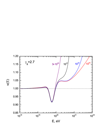
Figure 1: Upper panel: the trigger function $T(E)$ as function of energy. Lower panel: the distortion factor $\kappa(E)=J_{\rm kin}(E)/J_{\rm univ}(E)$ for $\gamma_{g}=2.7$ and different values of $E_{\rm max}$.

The kinetic equation (2) allows us a transparent interpretation of the spectral feature which appears at the energy $E_{\rm eq2}=6.0\times 10^{19}$ eV. At this energy one may limit the consideration to the present cosmological epoch $t\approx t_{0}$. As direct calculations show, the absorption term $-P(E)n_{p}(E)$ is then compensated with high accuracy by the regeneration term with $P(E,E^{\prime})$ in Eq. (2). At $E\approx E_{\rm eq2}$, the small CEL term (pair production) breaks this compensation, increasing the absorption term, and the spectrum acquires a dip. It is quite narrow because photo-pion energy losses increase with energy almost exponentially and at $E>E_{\rm eq2}$ the pair-production energy losses become too small. On the other hand, at $E<E_{\rm eq2}$ the photo-pion energy losses are too small, the spectrum is fully determined by pair-production energy losses, while the interference effect disappears.

Trigger mechanism.—Prior to presenting exact numerical calculations we shall study semi-quantitatively the triggering mechanism, responsible for the second dip. One can rearrange the first three terms on the rhs of Eq. (2) into $P_{\rm eff}(E,t)=P(E,t)+P_{\rm cont}(E,t)$ with

$$P_{\rm cont}(E,t)=2H(t)-\frac{\partial b(E,t)}{\partial E}$$ (4)

$$-\left[\frac{b_{\rm pair}(E,t)}{E}+H(t)\right]\frac{\partial\ln n(E,t)}{\partial\ln E}\,.$$

It is the term $P_{\rm cont}(E,t)$ that breaks the above-mentioned compensation between absorption and regeneration terms in Eq. (2), triggering thereby the modification of $n_{\rm kin}(E,t)$.

It is convenient to introduce the auxiliary trigger function $T(E)$ defined at $t=t_{0}$ as

$$T(E)=\left\{\begin{array}[]{ll}P_{\rm eff}(E)/P_{\rm cont}(E){}&{\rm for}~{}~{}E\leq E_{c}\\ P_{\rm eff}(E)/P(E){}&{\rm for}~{}~{}E\geq E_{c},\end{array}\right.$$ (5)

where $E_{c}=6.1\times 10^{19}$ eV is determined from the condition $P(E)=P_{\rm cont}(E)$ and is approximately equal to $E_{\rm eq2}$. The trigger function describes how $P_{\rm eff}(E)$ is changing from $P_{\rm cont}(E)$ at $E\ll E_{c}$, where $T(E)=1$, to $P(E)$ at $E\gg E_{c}$, where $T(E)=1$ as well. As long as $T(E)\approx 1$, there is no interference between pair-production and pion-production terms, and the ordinary solutions are valid. At $E=E_{c}$, $T(E)$ reaches its maximum and $P_{\rm eff}(E_{c})$, being noticeably larger than $P(E)$, breaks the compensation between absorption and regeneration terms in Eq. (2), making absorption larger. As a result, $n_{\rm kin}(E)$ decreases around $E_{c}$. The trigger function is plotted in Fig. 1. It reaches its maximum $T(E)=2$ at $E=E_{c}\approx 6.1\times 10^{19}$ eV. As explained above $n_{\rm kin}(E)$ must have a local minimum at this energy. The triggering mechanism predicts that the position of the dip minimum $E_{\rm 2dip}$ does not depend on $\gamma_{g}$ and $E_{\rm max}$ and these predictions are confirmed by our numerical calculations. The shape of $n_{\rm kin}(E)$ is expected to be similar to the shape of the trigger function $T(E)$ and this expectation is also confirmed by numerical calculations (see Fig. 1).

Numerical solutions.—We next discuss the second dip using numerical solutions of the kinetic equation (2). As mentioned above, the first dip is distinctly seen in the energy dependence of the modification factor $\eta(E)=J_{p}(E)/J_{p}^{\rm unm}(E)$. Similarly, the second dip is well seen, when the spectrum is described by a distortion factor, defined as $\kappa(E)=J_{\rm kin}(E)/J_{\rm univ}(E)$, where $J_{\rm univ}(E)$ is the universal spectrum from Eq. (1). We emphasize that the correct prediction for the measured spectrum is given by the kinetic equation (2), while the universal spectrum, used as a reference spectrum, is obtained in the CEL approximation and as such does not include the interference between pair and pion production. The calculated distortion factor is shown in the lower panel of Fig. 1 for $\gamma_{g}=2.7$ and four values of $E_{\rm max}$. The second dip is clearly seen. Its minimum is given by $E_{\rm 2dip}=6.3\times 10^{19}$ eV in good agreement with the prediction of the triggering mechanism. The width of the dip also agrees well with that of the trigger function $T(E)$. The independence of the spectral shape of the dip from the numerical value of $E_{\rm max}$, seen in Fig. 1, is another prediction of the triggering mechanism.

The distortion factor $\kappa$ does not return to unity after the second dip, but continues to grow for $E\gg E_{c}$. This deviation from unity is explained by fluctuations in photo-pion interactions. For $E\to E_{\rm max}$, the ratio $\kappa=J_{\rm kin}(E)/J_{\rm cont}(E)\to\infty$: At these energies Eq. (2) becomes stationary,

$$-P(E)n_{p}(E)+\int_{E}^{E_{\max}}\!\!\!\!dE^{\prime}P(E^{\prime},E)n_{p}(E^{\prime})+Q_{\rm gen}(E)=0\,.$$

When $E$ approaches $E_{\rm max}$, the regeneration term disappears, and one obtains $n_{\rm kin}(E_{\rm max})=Q_{\rm gen}(E_{\rm max})/P(E_{\rm max})$, remaining finite at $E_{\rm max}$. Using the CEL approximation, the equation reads

$$\partial/\partial E~{}[b_{\rm tot}(E)n_{p}(E)]+Q_{\rm gen}(E)=0\,.$$ (6)

For $E\to E_{\rm max}$, $n_{\rm cont}(E)\propto(E_{\rm max}-E)/E_{\rm max}\to 0$ and hence $\kappa(E_{\rm max})=n_{\rm kin}(E_{\rm max})/n_{\rm cont}(E_{\rm max})\to\infty$. The explosive behavior of the distortion factor for $E\to E_{\rm max}$ reflects the different limiting density of $n_{p}(E)$ in the kinetic and CEL equations. This result has a clear physical meaning. A particle has a finite probability to travel a finite distance without losing energy. While the kinetic equation describes correctly this effect, in the CEL approximation particles lose energy for any distance traversed, however small it may be. This influences the ratio $n_{\rm kin}(E)/n_{\rm cont}(E)$ at all energies close enough to $E_{\rm max}$ as can be seen in Fig. 1.

We have obtained one more proof for the energy-losses interference as the origin of the second dip. For this we have calculated the distortion factor in a toy model in which pair production and adiabatic energy losses were switched off. Then the interference term must disappear together with the second dip. The numerical calculations have confirmed this prediction for different $\gamma_{g}$ and $E_{\rm max}$.

In Fig. 2, the distortion factor is shown for different values of $\gamma_{g}$. One may observe the universality of the second dip with respect to variations of the spectral index, as expected from the triggering mechanism. We have performed these calculations using the FP equation.

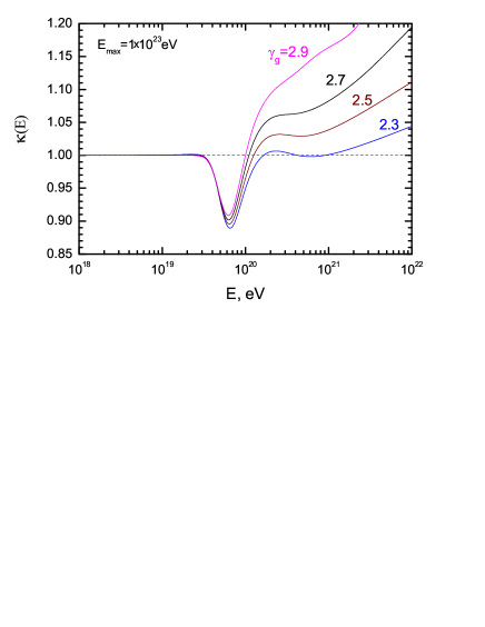
Figure 2: The distortion factor $\kappa$ as function of $E$ for $E_{\rm max}=1\times 10^{23}$ eV and different values of the spectral index $\gamma_{g}$.

Figures 1 and  2 show that the second dip is not sensitive to the exact values of $\gamma_{g}$ and $E_{\rm max}$. This implies also that a distribution of $\gamma_{g}$ and $E_{\max}$ values does not change the shape and position of the dip. Moreover, the cosmological evolution of sources is negligible at the energy of the second dip. The presence of nuclei primaries affects the second dip only for an extreme assumption about the fraction of nuclei. Light nuclei are photo-disintegrated at this energy and only the heaviest nuclei like Al and Fe survive. Their fraction at the production should be higher than 20% in order to hide the second dip mod .

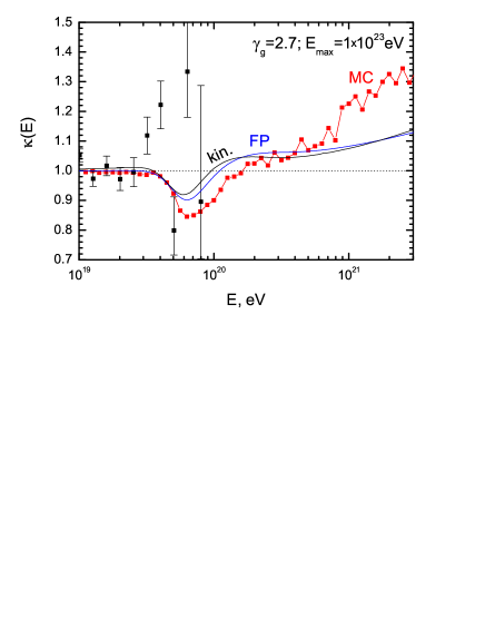
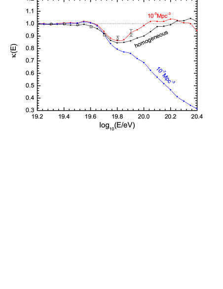
Figure 3: Top: The distortion factor calculated for $E_{\rm max}=1\times 10^{23}$ eV and $\gamma_{g}=2.7$ using the kinetic equation (curve ’kin’), the Fokker-Planck equation (curve ’FP’) and Monte Carlo calculations (curve ’MC’) for a homogeneous source distribution together the AGASA data with error bars reduced by a factor 3. Bottom: The distortion factor for a discrete source distribution, $n_{s}=10^{-5}~{}{\rm Mpc}^{-3}$, inspired by small-scale clustering, and $n_{s}=10^{-7}~{}{\rm Mpc}^{-3}$.

As our final test for the second dip we calculate the spectrum with a Monte Carlo (MC) simulation. The result of a MC simulation must coincide with the solution of the kinetic equation, if all relevant parameters of the problem are identical and when the number of MC runs tends to infinity. In our case, equal conditions means a homogeneous source distribution, the same generation spectra and $E_{\rm max}$ as well as identical $p\gamma$ interactions. We run the Monte Carlo simulation as described in Ref. KS using SOPHIA Sophia for the photo-pion interactions, while in the kinetic equation approach the calculations from Ref. BGG were used. As long as only average energy losses are concerned, the results of both works coincide very well (see BGG for a comparison). However, already small differences in the modeling of (differential) cross sections of order of a few percent can result in sizable variations of the distortion factor $\kappa$. Numerical errors in the calculations are another source of possible discrepancies. In Fig. 3 (top), we compare the distortion factors calculated with the kinetic equation, FP equation and MC methods for an homogeneous source density. The narrow second dip with minimum at $E_{\rm 2dip}=6.3\times 10^{19}$ eV is present in all calculations with small differences in shapes. The points from MC simulation are connected by straight lines, which helps to see the statistical uncertainties present especially at high energies.

We have also performed MC calculations for a discrete distribution of the sources using the values $n_{s}=10^{-5}~{}{\rm Mpc}^{-3}$ inspired by small-angle clustering and the very low density $n_{s}=10^{-7}~{}{\rm Mpc}^{-3}$, both shown in the bottom panel of Fig. 3. In the first case, the dip agrees well with those shown in the upper panel, while in the latter case the large distance $\sim 200$ Mpc to the nearest sources results in an early, very steep GZK cutoff that covers up the second dip.

We have compared these calculations with the AGASA data AG . The experimental distortion factors are obtained dividing the observed flux by the universal flux and normalizing the distortion factor at low energies to $\kappa=1$. We have diminished the true AGASA error bars by a factor three to give an impression of the potential of the Pierre Auger Observatory (PAO) to observe the second dip. This factor corresponds to a factor 10 improvement in statistics of PAO compared to AGASA. Even if the two data points at $4\times 10^{19}$ eV and $6\times 10^{19}$ eV would lie exactly on the predicted dip (this is quite possible for the true AGASA error bars), the large error bars in the PAO data will prevent a reliable conclusion on the presence of the second dip. The second dip is expected to be seen in the future JEM-EUSO space experiment EUSO , which will have a 100 times higher statistics than Auger (see bottom panel of Fig. 3). However, this expectation depends critically on the final energy threshold of this experiment, which is currently estimated as $5\times 10^{19}$ eV but is planned to be lowered EUSO . The second dip may be used as energy calibrator for this experiment, but accurate MC detector simulations are needed for this conclusion.

Conclusions.—We have found a new signature of the interactions of extragalactic UHE protons with the CMB radiation—the second dip. It is explained by the interference of pair and photo-pion production and has the shape of a narrow and shallow dip. The second dip is not seen if the admixture of nuclei heavier than Al in the generation flux is larger than 20% and if the space density of the sources is extremely small. The observation of the second dip is challenging for present experiments such as the PAO and requires future high-statistic cosmic ray detectors. Combined with the steepening of the UHECR spectrum, its observation provides an unambiguous signature of the GZK effect.

Acknowledgments—We gratefully acknowledge the participation of Svetlana Grigorieva at the early stage of this work. We thank ILIAS-TARI for access to the LNGS research infrastructure and for financial support through EU contract RII-CT-2004-506222.

References

- (1) K. Greisen, Phys. Rev. Lett. 16, 748 (1966); G. T. Zatsepin and V. A. Kuzmin, Pisma Zh. Experim. Theor. Phys. 4, 114 (1966) [JETP Lett. 4, 78 (1966)].
- (2) C. T. Hill and D. N. Schramm, Phys. Rev. D 31, 564 (1985).
- (3) V. S. Berezinsky and S. I. Grigorieva, Astron. Astrophys. 199, 1 (1988).
- (4) T. Stanev et al., Phys. Rev. D 62, 093005 (2000) [astro-ph/0003484].
- (5) V. Berezinsky, A. Z. Gazizov and S. I. Grigorieva, Phys. Lett. B 612, 147 (2005) [astro-ph/0502550].
- (6) M. Blanton, P. Blasi and A. V. Olinto, Astropart. Phys. 15, 275 (2001) [astro-ph/0009466].
- (7) V. Berezinsky, A. Z. Gazizov and S. I. Grigorieva, Phys. Rev. D 74, 043005 (2006) [hep-ph/0204357 v1].
- (8) R. Aloisio and V. Berezinsky, Astrophys. J. 612, 900 (2004) [astro-ph/0403095].
- (9) M. Kachelrieß and D. Semikoz, Astropart. Phys. 23, 486 (2005) [astro-ph/0405258].
- (10) A. Mücke et al., Comput. Phys. Commun. 124, 290 (2000) [astro-ph/9903478].
- (11) K. Shinozaki and M. Teshima, Nucl. Phys. B (Proc. Suppl.) 136, 18 (2004).
- (12) For a figure with the modification factor for He and Fe see R. Aloisio et al., astro-ph/0608219.
- (13) F. Kajino (JEM-EUSO collaboration), talk at 4th Korean Astrophysics Workshop, Daejeon, May 17-19, 2006, http://sirius.cnu.ac.kr/kaw4/presentations.htm