Infrared Counterparts to Chandra X-Ray Sources in the Antennae

Abstract

We use deep $J$ ($1.25\ \mu$m) and $K_{s}$ ($2.15\ \mu$m) images of the Antennae (NGC 4038/9) obtained with the Wide-field InfraRed Camera on the Palomar 200-inch telescope, together with the Chandra X-ray source list of Zezas et al. (2002a), to search for infrared counterparts to X-ray point sources. We establish an X-ray/IR astrometric frame tie with $\sim 0\farcs 5$ rms residuals over a $\sim 4\farcm 3$ field. We find 13 “strong” IR counterparts brighter than $K_{s}=17.8$ mag and $<1\farcs 0$ from X-ray sources, and an additional 6 “possible” IR counterparts between $1\farcs 0$ and $1\farcs 5$ from X-ray sources. Based on a detailed study of the surface density of IR sources near the X-ray sources, we expect only $\sim 2$ of the “strong” counterparts and $\sim 3$ of the “possible” counterparts to be chance superpositions of unrelated objects.

Comparing both strong and possible IR counterparts to our photometric study of $\sim 220$ IR clusters in the Antennae, we find with a $>$ 99.9% confidence level that IR counterparts to X-ray sources are $\Delta M_{K_{s}}\sim 1.2$ mag more luminous than average non-X-ray clusters. We also note that the X-ray/IR matches are concentrated in the spiral arms and “overlap” regions of the Antennae. This implies that these X-ray sources lie in the most “super” of the Antennae’s Super Star Clusters, and thus trace the recent massive star formation history here. Based on the $N_{H}$ inferred from the X-ray sources without IR counterparts, we determine that the absence of most of the “missing” IR counterparts../../../ASTRO-PH/ is not due to extinction, but that these sources are intrinsically less luminous in the IR, implying that they trace a different (possibly older) stellar population. We find no clear correlation between X-ray luminosity classes and IR properties of the sources, though small-number statistics hamper this analysis.

1 Introduction

Recently, high resolution X-ray images using Chandra have revealed 49 point sources in the Antennae (Zezas et al., 2002a). We will assume a distance to the Antennae of 19.3 Mpc (for $H_{0}$=75 km s^-1 Mpc^-1), which implies 10 sources have X-ray luminosities greater than $10^{39}$ ergs s^-1. Considering new observations of red giant stars in the Antennae indicate a distance of 13.8 Mpc (Saviane et al., 2004), we point out this ultraluminous X-ray source population could decrease by roughly a half. Typically, masses of black holes produced from standard stellar evolution are less than $\sim 20$ $M_{\odot}$ (e.g., Fryer & Kalogera, 2001). The Eddington luminosity limit implies that X-ray luminosities $>10^{39}$ ergs s^-1 correspond to higher-mass objects not formed from a typical star. Several authors (e.g., Fabbiano, 1989; Zezas, Georgantopoulos, & Ward, 1999; Roberts & Warwick, 2000; Makishima et al., 2000) suggest these massive ($10\sbond 1000$ $M_{\sun}$) compact sources outside galactic nuclei are intermediate mass black holes (IMBHs), a new class of BHs. While IMBHs could potentially explain the observed high luminosities, other theories exist as well, including beamed radiation from a stellar mass BH (King et al., 2001); super-Eddington accretion onto lower-mass objects (e.g., Moon, Eikenberry, & Wasserman, 2003; Begelman, 2002); or supernovae exploding in dense environments (Plewa, 1995; Fabian & Terlevich, 1996).

Compact objects tend to be associated with massive star formation, which is strongly suspected to be concentrated in young stellar clusters (Lada & Lada, 2003). Massive stars usually end their lives in supernovae, producing a compact remnant. This remnant can be kicked out of the cluster due to dynamical interactions, stay behind after the cluster evaporates, or remain embedded in its central regions. This last case is of particular interest to us as the compact object is still in situ, allowing us to investigate its origins via the ambient cluster population. The potential for finding such associations is large in the Antennae due to large numbers of both X-ray point sources and super star clusters; a further incentive for studying these galaxies.

In Brandl et al. (2005, henceforth Paper I) we presented $J$ and $K_{s}$ photometry of $\sim 220$ clusters in the Antennae. Analysis of ($J-K_{s}$) colors indicated that many clusters in the overlap region suffer from 9–10 mag of extinction in the $V$-band. This result contrasts with previous work by Whitmore & Zhang (2002) who associated optical sources with radio counterparts in the Antennae (Neff & Ulvestad, 2000) and argued that extinction is not large in this system. Here, we continue our analysis of these Antennae IR images by making a frame-tie between the IR and Chandra X-ray images from Fabbiano, Zezas, & Murray (2001). Utilizing the similar dust-penetrating properties of these wavelengths, we demonstrate the power of this approach to finding counterparts to X-ray sources. By comparing the photometric properties of clusters with and without X-ray counterparts, we seek to understand the cluster environments of these X-ray sources. In §2 we discuss the IR observations of the Antennae. §3 explains our matching technique and the photometric properties of the IR counterparts. We conclude with a summary of our results in §4.

2 Observations and Data Analysis

2.1 Infrared Imaging

We obtained near-infrared images of NGC 4038/9 on 2002 March 22 using the Wide-field InfraRed Camera (WIRC) on the Palomar 5-m telescope. At the time of these observations, WIRC had been commissioned with an under-sized HAWAII-1 array (prior to installation of the full-sized HAWAII-2 array in September 2002), providing a $\sim 4.7\times 4.7$-arcminute field of view with $\sim 0\farcs 25$ pixels (“WIRC-1K” – see Wilson et al. (2003) for details). Conditions were non-photometric due to patches of cloud passing through. Typical seeing-limited images had stellar full-width at half-maximum of $1\farcs 0$ in $K_{s}$ and $1\farcs 3$ in $J$. We obtained images in both the $J$- ($1.25\mu$m) and $K_{s}$-band ($2.15\mu$m) independently. The details of the processing used to obtain the final images are given in Paper 1.

2.2 Astrometric Frame Ties

The relative astrometry between the X-ray sources in NGC 4038/9 and images at other wavelengths is crucial for successful identification of multi-wavelength counterparts. Previous attempts at this have suffered from the crowded nature of the field and confusion between potential counterparts Zezas et al. (2002b). However, the infrared waveband offers much better hopes for resolving this issue, due to the similar dust-penetrating properties of photons in the Chandra and $K_{s}$ bands. (See also Brandl et al. (2005) for a comparison of IR extinction to the previous optical/radio extinction work of Whitmore & Zhang (2002).) We thus proceeded using the infrared images to establish an astrometric frame-tie, i.e. matching Chandra coordinates to IR pixel positions.

As demonstrated by Bauer et al. (2000), we must take care when searching for X-ray source counterparts in crowded regions such as the Antennae. Therefore, our astrometric frame-tie used a unique approach based on solving a two-dimensional linear mapping function relating right ascension and declination coordinates in one image with x and y pixel positions in a second image. The solution is of the form:

$$r_{1}=ax_{1}+by_{1}+c,$$ (1)

$$d_{1}=dx_{1}+dy_{1}+f$$ (2)

Here $r_{1}$ and $d_{1}$ are the right ascension and declination, respectively, for a single source in one frame corresponding to the $x_{1}$ and $y_{1}$ pixel positions in another frame. This function considers both the offset and rotation between each frame. Since we are interested in solving for the coefficients $a$–$f$, elementary linear algebra indicates we need six equations or three separate matches. Therefore, we need at least three matches to fully describe the rms positional uncertainty of the frame-tie.

We first used the above method to derive an approximate astrometric solution for the WIRC $K_{s}$ image utilizing the presence of six relatively bright, compact IR sources which are also present in images from the 2-Micron All-Sky Survey (2MASS). We calculated pixel centroids of these objects in both the 2MASS and WIRC images, and used the 2MASS astrometric header information to convert the 2MASS pixel centroids into RA and Dec. These sources are listed in Table 1. Applying these six matches to our fitting function we found a small rms positional uncertainty of $0\farcs 2$, which demonstrates an accurate frame-tie between the 2MASS and WIRC images.

Using the 2MASS astrometric solution as a baseline, we identified seven clear matches between Chandra and WIRC sources, which had bright compact IR counterparts with no potentially confusing sources nearby (listed in Table 2). We then applied the procedure described above, using the Chandra coordinates listed in Table 1 of Zezas et al. (2002a) (see that reference for details on the Chandra astrometry) and the WIRC pixel centroids, and derived the astrometric solution for the IR images in the X-ray coordinate frame. For the 7 matches, we find an rms residual positional uncertainty of $\sim 0\farcs 5$ which we adopt as our $1\sigma$ position uncertainty. We note that the positional uncertainty is an entirely empirical quantity. It shows the achieved uncertainty in mapping a target from one image reference frame to the reference frame in another band, and automatically incorporates all contributing sources of uncertainty in it. These include, but are not limited to, systematic uncertainties (i.e. field distortion, PSF variation, etc. in both Chandra and WIRC) and random uncertainties (i.e. centroid shifts induced by photon noise, flatfield noise, etc. in both Chandra and WIRC). Thus, given the empirical nature of this uncertainty, we expect it to provide a robust measure of the actual mapping error – an expectation which seems to be borne out by the counterpart identification in the following section.

To further test the accuracy of our astrometric solution we explored the range in rms positional uncertainties for several different frame-ties. Specifically we picked ten IR/X-ray matches separated by $<$1$\arcsec$, which are listed in Table 3 (see §3.1). Of these ten we chose 24 different combinations of seven matches resulting in 24 unique frame-ties. Computing the rms positional uncertainty for each we found a mean of 0$\farcs$4 with a 1$\sigma$ uncertainty of 0$\farcs$1. Considering the rms positional uncertainty for the frame-tie used in our analysis falls within 1$\sigma$ of this mean rms, this indicates we made an accurate astrometric match between the IR and X-ray.

2.3 Infrared Photometry

We performed aperture photometry on 222 clusters in the $J$-band and 221 clusters in the $K_{s}$-band (see also Paper 1). We found that the full width at half maximum (FWHM) was 3.5 pixels ($0\farcs 9$) in the $K_{s}$ image and 4.6 pixels ($1\farcs 2$) in the $J$ band. We used a photometric aperture of 5-pixel radius in $K_{s}$ band, and 6-pixel radius in $J$ band, corresponding to $\sim 3\sigma$ of the Gaussian PSF.

Background subtraction is both very important and very difficult in an environment such as the Antennae due to the brightness and complex structure of the underlying galaxies and the plethora of nearby clusters. In order to address the uncertainties in background subtraction, we measured the background in two separate annuli around each source: one from 9 to 12 pixels and another from 12 to 15 pixels. Due to the high concentration of clusters, crowding became an issue. To circumvent this problem, we employed the use of sky background arcs instead of annuli for some sources. These were defined by a position angle and opening angle with respect to the source center. All radii were kept constant to ensure consistency. In addition, nearby bright sources could shift the computed central peak position by as much as a pixel or two. If the centroid position determined for a given source differed significantly ($>1$ pixel) from the apparent brightness peak due to such contamination, we forced the center of all photometric apertures to be at the apparent brightness peak. For both annular regions, we calculated the mean and median backgrounds per pixel.

Multiplying these by the area of the central aperture, these values were subtracted from the flux measurement of the central aperture to yield 4 flux values for the source in terms of DN. Averaging these four values provided us with a flux value for each cluster. We computed errors by considering both variations in sky background, $\sigma_{sky}$, and Poisson noise, $\sigma_{adu}$. We computed $\sigma_{sky}$ by taking the standard deviation of the four measured flux values. We then calculated the expected Poisson noise by scaling DN to $e^{-}$ using the known gain of WIRC (2 $e^{-1}$ DN^-1, Wilson et al., 2003) and taking the square root of this value. We added both terms in quadrature to find the total estimated error in photometry.

We then calibrated our photometry using the bright 2MASS star in Table 1.

3 Results and Discussion

3.1 Identification of IR Counterparts to Chandra Sources

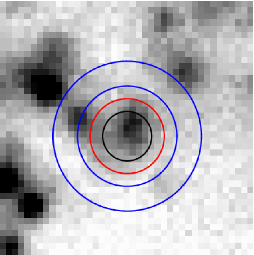
Figure 1: IR counterpart to X-36 overlaid with areas of positional uncertainty centered on the X-ray source position. Black: 1$\farcs$0 radius circle for strong sources, red: 1$\farcs$0 – 1$\farcs$5 annulus for possible sources, and blue: 2$\farcs$0 – 3$\farcs$0 annulus used to estimate background source contamination.

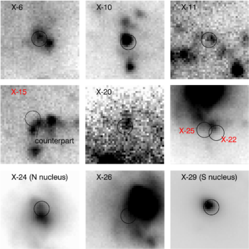
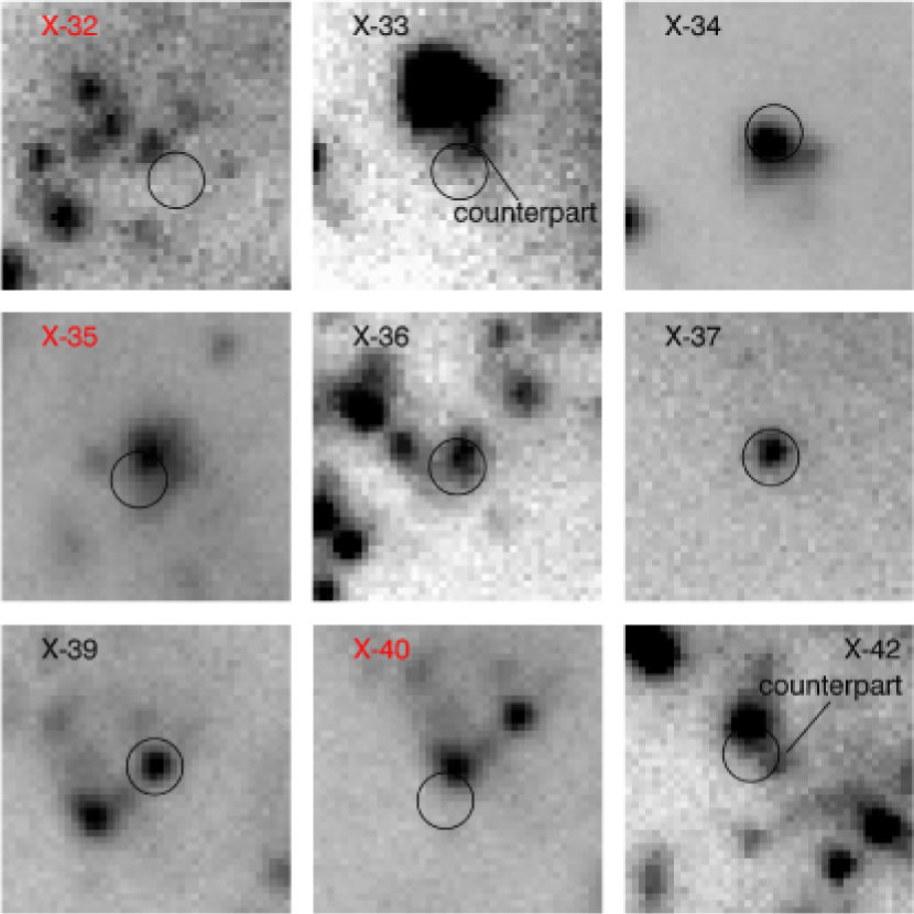
Figure 3: Subimages highlighting X-ray positions for all X-rays sources with IR counterparts. Positional error circles are $1\farcs 0$ in radius. Image field-of-view is $10\farcs 0\times 10\farcs 0$ and north is up. We label “strong” matches in black and “possible” matches in red.

We used the astrometric frame-tie described above to identify IR counterpart candidates to Chandra X-ray sources in the WIRC $K_{s}$ image. We restricted our analysis to sources brighter than $K_{s}\sim 19.4$ mag. This is our $K_{s}$ sensitivity limit which we define in our photometric analysis below (see §3.2.1). Using the $0\farcs 5$ rms positional uncertainty of our frame-tie, we defined circles with 2$\sigma$ and 3$\sigma$ radii around each Chandra X-ray source where we searched for IR counterparts (Figure 1). If an IR source lay within a $1\farcs 0$ radius ($2\sigma$) of an X-ray source, we labeled these counterparts as “strong”. Those IR sources between $1\farcs 0$ and $1\farcs 5$ ($2-3\sigma$) from an X-ray source we labeled as “possible” counterparts. We found a total of 13 strong and 6 possible counterparts to X-ray sources in the Antennae. These sources are listed in Table 3 and shown in Figure 3. Of the 19 X-ray sources with counterparts, two are the nuclei (Zezas et al., 2002a), one is a background quasar (Clark et al., 2005), and two share the same IR counterpart. Therefore, in our analysis of cluster properties, we only consider the 15 IR counterparts that are clusters. (While X-42 has two IR counterparts, we chose the closer, fainter cluster for our analysis.)

We then attempted to estimate the level of “contamination” of these samples due to chance superposition of unrelated X-ray sources and IR clusters. This estimation can be significantly complicated by the complex structure and non-uniform distribution of both X-ray sources and IR clusters in the Antennae, so we developed a simple, practical approach. Given the $<0\farcs 5$ rms residuals in our relative astrometry for sources in Table 2, we assume that any IR clusters lying in a background annulus with radial size of $2\farcs 0$–$3\farcs 0$ ($4-6\sigma$) centered on all X-ray source positions are chance alignments, with no real physical connection (see Figure 1). Dividing the total number of IR sources within the background annuli of the 49 X-ray source positions by the total area of these annuli, we find a background IR source surface density of 0.02 arcsecond^-2 near Chandra X-ray sources. Multiplying this surface density by the total area of all “strong” regions ($1\farcs 0$ radius circles) and “possible” regions ($1\farcs 0$ – $1\farcs 5$ annuli) around the 49 X-ray source positions, we estimated the level of source contamination contributing to our “strong” and “possible” IR counterpart candidates. We expect two with a $1\sigma$ uncertainty of +0.2/-0.1 of the 13 “strong” counterparts to be due to chance superpositions, and three with a $1\sigma$ uncertainty of +0.5/-0.3 of the six “possible” counterparts to be chance superpositions.

This result has several important implications. First of all, it is clear that we have a significant excess of IR counterparts within $1\farcs 0$ of the X-ray sources – 13, where we expect only two in the null hypothesis of no physical counterparts. Even including the “possible” counterparts out to $1\farcs 5$, we have a total of 19 counterparts, where we expect only five from chance superposition. Secondly, this implies that for any given “strong” IR counterpart, we have a probability of $\sim$ 85% ($11/13$ with a $1\sigma$ uncertainty of 0.3) that the association with an X-ray source is real. Even for the “possible” counterparts, the probability of true association is $\sim$50%. These levels of certainty are a tremendous improvement over the X-ray/optical associations provided by Zezas et al. (2002b), and are strong motivators for follow-up multi-wavelength studies of the IR counterparts. Finally, we can also conclude from strong concentration of IR counterparts within $\sim 1\arcsec$ of X-ray sources that the frame tie uncertainty estimates described above are reasonable.

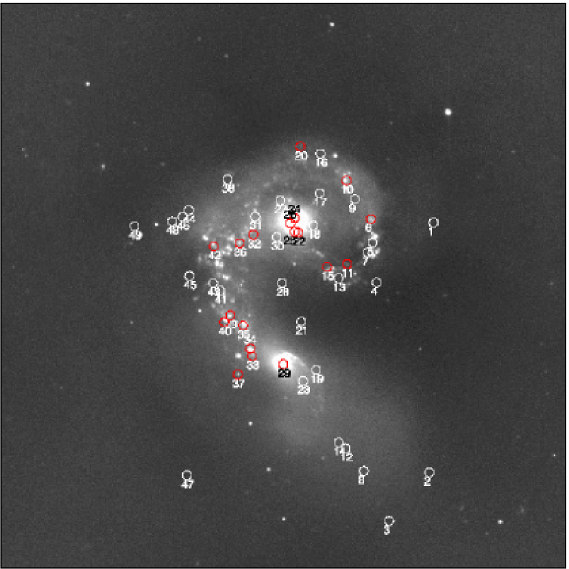
Figure 2: $K_{s}$-band image of the Antennae showing positions of X-ray sources. The field-of-view is $4\farcs 3\times 4\farcs 3$. Red circles designate those sources with IR counterparts. Notice these tend to reside in the spiral arms and bridge region between the galaxies.

Figure 2 is a $4\farcm 3\times 4\farcm 3$ $K_{s}$ image of the Antennae with X-ray source positions overlaid. We designate those X-ray sources with counterparts using red circles. Notice that those sources with counterparts lie in the spiral arms and bridge region of the Antennae. Since these regions are abundant in star formation, this seems to indicate many of the X-ray sources in the Antennae are tied to star formation in these galaxies.

3.2 Photometric Properties of the IR Counterparts

3.2.1 Color Magnitude Diagrams

Using the 219 clusters that had both $J$ and $K_{s}$ photometry, we made $(J-K_{s})$ versus $K_{s}$ color magnitude diagrams (Figure 4). We estimated our sensitivity limit by first finding all clusters with signal-to-noise $\sim 5\sigma$. The mean $J$ and $K_{s}$ magnitudes for these clusters were computed separately and defined as cutoff values for statistical analyzes. This yielded 19.0 mag in $J$ and 19.4 mag in $K_{s}$. We note that the X-ray clusters are generally bright in the IR compared to the general population of clusters. While the IR counterpart for one X-ray source (X-32) falls below our $J$-band sensitivity limit, its $K_{s}$ magnitude is still above our $K_{s}$ cutoff. Therefore, we retained this source in our analysis.

We then broke down the X-ray sources into three luminosity classes (Figure 4). We took the absorption-corrected X-ray luminosities, $L_{X}$, as listed in Table 1 of Zezas et al. (2002a) for all sources of interest. These luminosities assumed a distance to the Antennae of 29 Mpc. We used 19.3 Mpc (for $H_{0}$=75 km s^-1 Mpc^-1) instead and so divided these values by 2.25 as suggested in Zezas et al. (2002a). We defined the three X-ray luminosities as follows: Low Luminosity X-ray sources (LLX’s) had $L_{X}$ $<$ 3$\times$$10^{38}$ ergs s^-1, High Luminosity X-ray sources (HLX’s) were between $L_{X}$ of 3$\times 10^{38}$ergs s^-1 and 1$\times 10^{39}$ ergs s^-1, while $L_{X}$ $>$ 1$\times 10^{39}$ ergs s^-1 were Ultra-Luminous X-ray Sources (ULX’s). In Figure 4 we designate each IR counterpart according to the luminosity class of its corresponding X-ray source. There does not appear to be a noticeable trend in the IR cluster counterparts between these different groupings.

3.2.2 Absolute K Magnitudes

To further study the properties of these IR counterparts, we calculated $M_{K_{s}}$ for all IR clusters. We calculated reddening using the observed colors, $(J-K_{s})_{obs}$, (hence forth the “color method”). Assuming all clusters are dominated by O and B stars, their intrinsic $(J-K_{s})$ colors are $\sim$0.2 mag. Approximating this value as 0 mag, this allowed us to estimate $A_{K_{s}}$ as $\simeq$ $(J-K_{s})_{obs}$/1.33 using the extinction law defined in Cardelli, Clayton, & Mathis (1989, hereafter CCM). Since these derived reddenings are biased towards young clusters, they will lead to an overestimate of $M_{K_{s}}$ for older clusters.

For IR counterparts to X-ray sources, we also computed X-ray-estimated $A_{K_{s}}$ using the column densities, $N_{H}$, listed in Table 5 of Zezas et al. (2002a). Here, $N_{H}$ is derived by fitting both a Power Law (PL) and Raymond-Smith (RS Raymond & Smith, 1977) model to the X-ray spectra. Using the CCM law, $A_{K_{s}}$ is defined as 0.12$A_{V}$. Taking $A_{V}$ = $5\times 10^{-22}$ mag cm² $N_{H}$, we could then derive $A_{K_{s}}$.

Then we compared $A_{K_{s}}$ calculated using the “color method” to $A_{K_{s}}$ found using the above two $N_{H}$ models. We found the “color method” matched closest to $N_{H}(PL)$ for all except one (the cluster associated with Chandra source 32 as designated in Zezas et al. (2002b)).

In Figure 5, we plot histograms of the distribution of $K_{s}$-band luminosity, $M_{K_{s}}$. Figure 5 displays all clusters as well as over plotting only those with X-ray counterparts. Notice that the clusters with associated X-ray sources look more luminous. To study whether this apparent trend in luminosity is real, we compared these two distributions using a two-sided Kolmogorov-Smirnov (KS) test. In our analysis, we only included clusters below $M_{K_{s}}$ $<$ -13.2 mag. Restricting our study to sources with “good” photometry, we first defined a limit in $K_{s}$, 18.2 mag, using the limiting $J$ magnitude, 19.0 mag as stated above, and, since the limit in $K_{s}$ is a function of cluster color, the median $(J-K_{s})$ of 0.8 mag. Subtracting the distance modulus to the Antennae, 31.4 mag, from this $K_{s}$ limit, we computed our cutoff in $M_{K_{s}}$. Since all clusters with X-ray sources fall below this cutoff, our subsample is sufficient to perform a statistical comparison.

The KS test yielded a D-statistic of 0.37 with a probability of $3.2\times 10^{-2}$ that the two distributions of clusters with and without associated X-ray sources are related. Considering the separate cluster populations as two probability distributions, each can be expressed as a cumulative distribution. The D-statistic is then the absolute value of the maximum difference between each cumulative distribution. This test indicates that those clusters with X-ray counterparts are more luminous than most clusters in the Antennae.

3.2.3 Cluster Mass Estimates

Whitmore et al. (1999) found 70% of the bright clusters observed with the Hubble Space Telescope have ages $<$20 Myr. Therefore, in this study we will assume all clusters are typically the same age, $\sim$20 Myr. This allows us to make the simplifying assumption that cluster mass is proportional to luminosity and ask: Does the cluster mass affect the propensity for a given progenitor star to produce an X-ray binary? We estimated cluster mass using $K_{s}$ luminosity ($M_{K_{s}}$). Since cluster mass increases linearly with flux (for an assumed constant age of all clusters), we converted $M_{K_{s}}$ to flux. Using the data as binned in the $M_{K_{s}}$ histogram (Figure 5), we calculated an average flux per bin. By computing the fraction of number of clusters per average flux, we are in essence asking what is the probability of finding a cluster with a specific mass. Since those clusters with X-ray sources are more luminous, we expect a higher probability of finding an X-ray source in a more massive cluster. As seen in Figure 6, this trend does seem to be true. Applying a KS-test between the distributions for all clusters and those associated with X-ray sources for clusters below the $M_{K_{s}}$ completeness limit defined in the previous section, we find a D-statistic of 0.66 and a probability of $7.2\times 10^{-3}$ that they are the same. Hence, the two distributions are distinct, indicating it is statistically significant that more massive clusters tend to contain X-ray sources.

While we assume all clusters are $\sim$20 Myr above, we note that the actual range in ages is $\sim$1–100 Myr (Whitmore et al., 1999). Bruzual-Charlot spectral photometric models (Bruzual & Charlot, 2003) indicate that clusters in this age range could vary by a factor of roughly 100 in mass for a given $K_{s}$ luminosity. Thus, we emphasize that the analysis above should be taken as suggestive rather than conclusive evidence, and note that in a future paper (Clark, et al. 2006, in preparation) we explore this line of investigation and the impacts of age variations on the result in depth.

3.2.4 Non-detections of IR Counterparts to X-ray Sources

To assess whether our counterpart detections were dependent of reddening or their intrinsic brightness, we found limiting values for $M_{K_{s}}$ for those X-ray sources without detected IR counterparts. We achieved this by setting all clusters $K_{s}$ magnitudes equal to our completeness limit defined for the CMDs (19.4 mag; see §3.2.1) and then finding $M_{K_{s}(lim)}$ for each using $A_{K_{s}}$ calculated for that cluster. Since $M_{K_{s}(lim)}$ is theoretical and only depends on reddening, we could now find this limit for all X-ray sources using an $A_{K_{s}}$ estimated from the observed $N_{H}$ values. Thus we considered all IR counterparts (detections) and those X-ray sources without a counterpart (nondetections). If nondetections are due to reddening there should not exist a difference in $M_{K_{s}(lim)}$ between detections and nondetections. In contrast, if nondetections are intrinsically fainter, we expect a higher $M_{K_{s}(lim)}$ for these sources. In the case of detections, we considered reddening from both the “color method” and the $N_{H}(PL)$ separately. We could only derive nondetections using $N_{H}(PL)$ reddening. Figure 7 shows $M_{K_{s}(lim)}$ appears higher for all nondetections. To test if this observation is significant, we applied a KS-test to investigate whether detections and nondetections are separate distributions. We find a D-statistic of 0.82 and probability of $8.8\times 10^{-6}$ that these two distributions are the same using the “color method” for detections. Considering the $N_{H}(PL)$ reddening method for detections instead, the D-statistic drops to 0.48 and the probability increases to $3.9\times 10^{-2}$. Since both tests indicate these distributions are distinct, the observed high $M_{K_{s}(lim)}$ for nondetections seems to be real. This leads to the conclusion that these sources were undetected because they are intrinsically IR-faint, and that reddening does not play the dominant role in nondetections.

We summarize these statistics in Table 4. Here we calculated the mean $K_{s}$, $(J-K_{s})$, and $M_{K_{s}}$ for three different categories: 1) all clusters, 2) clusters only connected with X-ray sources, and 3) these clusters broken down by luminosity class. We also include uncertainties in each quantity. Notice that the IR counterparts appear brighter in $K_{s}$ and intrinsically more luminous than most clusters in the Antennae, although there is no significant trend in color. We also summarize the above KS-test results in Table 5.

4 Conclusions

We have demonstrated a successful method for finding counterparts to X-ray sources in the Antennae using IR wavelengths. We mapped Chandra X-ray coordinates to WIRC pixel positions with a positional uncertainty of $\sim 0\farcs 5$. Using this precise frame-tie we found 13 “strong” matches ($<1\farcs 0$ separation) and 5 “possible” matches ($1-1\farcs 5$ separation) between X-ray sources and IR counterparts. After performing a spatial and photometric analysis of these counterparts, we reached the following conclusions:

1. We expect only 2 of the 13 “strong” IR counterparts to be chance superpositions. Including all 19 IR counterparts, we estimated 5 are unrelated associations. Clearly, a large majority of the X-ray/IR associations are real.

2. The IR counterparts tend to reside in the spiral arms and bridge region between these interacting galaxies. Since these regions contain the heaviest amounts of star formation, it seems evident that many of the X-ray sources are closely tied to star formation in this pair of galaxies.

3. A $K_{s}$ vs. $(J-K_{s})$ CMD reveal those clusters associated with X-ray sources are brighter in $K_{s}$ but there does not seem to be a trend in color. Separating clusters by the X-ray luminosity classes of their X-ray counterpart does not reveal any significant trends.

4. Using reddening derived $(J-K_{s})$ colors as well as from X-ray-derived $N_{H}$, we found $K_{s}$-band luminosity for all clusters. A comparison reveals those clusters associated with X-ray sources are more luminous than most clusters in the Antennae. A KS-test indicates a significant difference between X-ray counterpart clusters and the general population of clusters.

5. By relating flux to cluster luminosity, simplistically assuming a constant age for all clusters, we estimated cluster mass. Computing the fraction of number of clusters per average flux, we estimated the probability of finding a cluster with a specific mass. We find more massive clusters are more likely to contain X-ray sources, even after we normalize by mass.

6. We computed a theoretical, limiting $M_{K_{s}}$ for all counterparts to X-ray sources in the Antennae using X-ray-derived reddenings. Comparing detections to non-detections, we found those clusters with X-ray source are intrinsically more luminous in the IR.

In a future paper exploring the effects of cluster mass on XRB formation rate (Clark, et al. 2006a, in preparation), we will investigate the effects of age on cluster luminosity and hence our cluster mass estimates. Another paper will extend our study of the Antennae to optical wavelengths (Clark, et al. 2006b, in preparation). Through an in depth, multi-wavelength investigation we hope to achieve a more complete picture of counterparts to several X-ray sources in these colliding galaxies.

Table 1: Common Sources Used for the 2MASS/WIRC Astrometric Frame Tie

Description	RA (2MASS)	Dec (2MASS)	$J$	$K_{s}$
Bright Star	12:01:47.90	-18:51:15.8	13.07(0.01)	12.77(0.01)
Southern Nucleus	12:01:53.50	-18:53:10.0	13.45(0.05)	12.50(0.03)
Cluster 1	12:01:51.66	-18:51:34.7	14.84(0.01)	14.24(0.01)
Cluster 2	12:01:50.40	-18:52:12.2	14.98(0.02)	14.06(0.01)
Cluster 3	12:01:54.56	-18:53:04.0	15.05(0.03)	14.27(0.02)
Cluster 4	12:01:54.95	-18:53:05.8	16.52(0.01)	14.66(0.01)

Table 2: Common Sources Used for the Chandra/WIRC Astrometric Frame Tie

Chandra Source ID	RA (Chandra)	Dec (Chandra)	$K_{s}$
6	12:01:50.51	$-$18:52:04.80	15.66(0.02)
10	12:01:51.27	$-$18:51:46.60	14.66(0.01)
24	12:01:52.99	$-$18:52:03.20	13.55(0.11)
29	12:01:53.49	$-$18:53:11.10	12.50(0.03)
34	12:01:54.55	$-$18:53:03.20	14.27(0.02)
36	12:01:54.81	$-$18:52:14.00	15.92(0.01)
37	12:01:54.98	$-$18:53:15.10	16.16(0.01)

Table 3: Potential IR Counterparts to Chandra X-Ray Sources

			$\Delta\alpha$	$\Delta\delta$
Chandra Src ID	RA	Dec	(arcsec)	(arcsec)	$J$	$K_{s}$
“Strong” Counterparts
6	12:01:50.51	-18:52:04.77	0.29	0.04	16.21(0.01)	15.66(0.02)
10	12:01:51.27	-18:51:46.58	0.24	0.31	15.57(0.01)	14.66(0.01)
11	12:01:51.32	-18:52:25.46	0.34	0.03	18.27(0.01)	17.37(0.08)
20	12:01:52.74	-18:51:30.06	0.11	0.38	18.48(0.04)	17.78(0.02)
24	12:01:52.99	-18:52:03.18	0.07	0.82	14.37(0.11)	13.55(0.11)
26	12:01:53.13	-18:52:05.53	0.27	0.87	15.95(0.01)	14.71(0.15)
29	12:01:53.49	-18:53:11.08	0.20	0.25	13.45(0.05)	12.50(0.03)
33	12:01:54.50	-18:53:06.82	0.11	0.99	16.71(0.08)	16.45(0.07)
34	12:01:54.55	-18:53:03.23	0.02	0.39	15.05(0.03)	14.27(0.02)
36	12:01:54.81	-18:52:13.99	0.11	0.50	16.60(0.03)	15.92(0.01)
37	12:01:54.98	-18:53:15.07	0.13	0.10	17.55(0.02)	16.16(0.01)
39	12:01:55.18	-18:52:47.50	0.18	0.03	17.10(0.07)	15.71(0.04)
42	12:01:55.65	-18:52:15.06	0.73	0.40	17.13(0.03)	16.27(0.06)
“Possible” Counterparts
15	12:01:51.98	-18:52:26.47	1.09	0.84	16.63(0.04)	15.95(0.02)
22	12:01:52.89	-18:52:10.03	0.70	1.20	15.77(0.01)	15.13(0.06)
25	12:01:53.00	-18:52:09.59	0.87	0.76	15.77(0.01)	15.13(0.06)
32	12:01:54.35	-18:52:10.31	0.92	1.39	20.30(0.45)	16.84(0.03)
35	12:01:54.77	-18:52:52.43	0.42	0.92	16.76(0.02)	14.88(0.04)
40	12:01:55.38	-18:52:50.53	0.61	1.24	16.21(0.02)	15.27(0.04)

Table 4: Summary of Potential IR Counterpart Properties.

Category	$\overline{K}$	$\sigma_{\overline{K}}$	$\overline{(J-K)}$	$\sigma_{\overline{(J-K)}}$	$\overline{M_{K_{s}}}$	$\sigma_{\overline{M_{K}}}$
all clusters	16.72	0.08	0.82	0.03	-15.33	0.09
X-ray sources	15.72	0.27	0.95	0.11	-16.30	0.35
LLX	15.85	0.36	0.84	0.11	-16.16	0.39
HLX	15.09	0.37	1.13	0.28	-17.14	0.54
ULX	16.82	0.55	0.88	0.02	-14.67	0.51

Table 5: Summary of KS-Test Results.

	Probability	D
$M_{K_{s}}$	$3.2\times 10^{-2}$	0.37
Cluster Mass	$9.6\times 10^{-2}$	0.40
$M_{K_{s}(lim)}$ (CM)	$8.8\times 10^{-6}$	0.82
$M_{K_{s}(lim)}$ (NH)	$3.9\times 10^{-2}$	0.48

Figure 4a: (a) $(J-K_{s})$ vs. $K_{s}$ CMD for all clusters with photometry. In each of the next three plots, the dotted line shows our cutoff for statistical analyzes. (b) Here clusters with X-ray counterparts are designated. Note that one IR counterpart falls below our sensitivity limit. Since its $K_{s}$ magnitude is still above our $K_{s}$ cutoff, we retained this source in our analysis. (c) These clusters are broken down by their luminosity class. LLX: $L_{X}$ $<$ 3$\times 10^{38}$ ergs s^-1, HLX: 3$\times 10^{38}$ ergs s^-1 $<$ $L_{X}$ $<$ 1$\times$$10^{39}$ergs s^-1, and ULX: $L_{X}$ $>$ 1$\times$$10^{39}$ ergs s^-1.

Figure 4b:

Figure 4c:

Figure 5: $M_{K_{s}}$ histogram for all clusters. Binned by 0.2 magnitudes. Dashed line shows cutoff for statistical analyzes.

Figure 6: This figure is the same as Figure 5, except that we have plotted $M_{K_{s}}$ versus the number of clusters per bin divided by the mean flux in that bin. Arguing that mass is proportional to flux, this graph shows the probability of finding a cluster with a given mass.

Figure 7: Theoretical, $M_{K(lim)}$ histograms for all X-ray sources with counterparts, detections, and those without, nondetections, using bins of 0.2 magnitudes. For detections, reddening computed using $N_{H}(PL)$ (top) and “color method” (bottom).

References

- Begelman (2002) Begelman, M. C. 2002, ApJ, 568, L97
- Brandl et al. (2005) Brandl, B. R. et al. 2005, ApJ, 635, 280
- Bruzual & Charlot (2003) Bruzual, G. & Charlot, S. 2003, MNRAS, 344, 1000
- Bauer et al. (2000) Bauer, F. E., Condon, J. J., Thuan, T. X., & Broderick, J. J. 2000, ApJS, 129, 547
- Cardelli, Clayton, & Mathis (1989) Cardelli, J. A., Clayton, G. C., & Mathis, J. S. 1989, ApJ, 345, 245
- Clark et al. (2005) Clark, D. M. et al. 2005, ApJ, 631, L109
- Fabbiano (1989) Fabbiano, G. 1989, ARA&A, 27, 87
- Fabbiano, Zezas, & Murray (2001) Fabbiano, G., Zezas, A., & Murray, S. S. 2001, ApJ, 554, 1035
- Fabian & Terlevich (1996) Fabian, A. C. & Terlevich, R. 1996, MNRAS, 280, L5
- Fryer & Kalogera (2001) Fryer, C. L., & Kalogera, V. 2001, ApJ, 554, 548
- Gehrels (1986) Gehrels, N. 1986, ApJ, 303, 336
- King et al. (2001) King, A. R, Davies, M. B., Ward, M. J., Fabbiano, G., & Elvis, M. 2001, ApJ, 552, L109
- Makishima et al. (2000) Makishima, K. et al. 2000, ApJ, 535, 632
- Moon, Eikenberry, & Wasserman (2003) Moon, D.-S., Eikenberry, S. S., & Wasserman, I. M. 2003, ApJ, 586, 1280
- Neff & Ulvestad (2000) Neff, S. G., & Ulvestad, J. S. 2000, AJ, 120, 670
- Lada & Lada (2003) Lada, C. J. & Lada, E. A. 2003, ARA&A, 41, 57
- Plewa (1995) Plewa, T. 1995, MNRAS, 275, 143
- Raymond & Smith (1977) Raymond, J. C. & Smith, B. W. 1977, ApJS, 35, 419
- Roberts & Warwick (2000) Roberts, T. P. & Warwick, R. S. 2000, MNRAS, 315, 98
- Saviane et al. (2004) Saviane, I., Hibbard, J. E., & Rich, R. M. 2004, IAUS, 217, 546
- Whitmore et al. (1999) Whitmore, B. C., Zhang, Q., Leitherer, C., Fall, S. M., Schweizer, F., & Miller, B. W. 1999, AJ, 118, 1551
- Whitmore & Zhang (2002) Whitmore, B. C. & Zhang, Q. 2002, AJ, 124, 1418
- Wilson et al. (2003) Wilson, J. C. et al. 2003, Proc. SPIE, 4841, 451
- Zezas, Georgantopoulos, & Ward (1999) Zezas, A. L., Georgantopoulos, I., & Ward, M. J. 1999, MNRAS, 308, 302
- Zezas et al. (2002a) Zezas, A., Fabbiano, G., Rots, A. H., & Murray, S. S. 2002a, ApJS, 142, 239
- Zezas et al. (2002b) Zezas, A., Fabbiano, G., Rots, A. H., & Murray, S. S. 2002b, ApJ, 577, 710