Chemical Abundance Analysis of the
Extremely Metal-Poor Star HE 1300$+$0157

Abstract

We present a detailed chemical abundance analysis of HE 1300$+$0157, a subgiant with $\mbox{[Fe/H]}=-3.9$. From a high-resolution, high-$S/N$ Subaru/HDS spectrum we find the star to be enriched in C ($\mbox{[C/Fe]}_{\rm 1D}\sim+1.4$) and O ($\mbox{[O/Fe]}_{\rm 1D}\sim+1.8$). With the exception of these species, HE 1300$+$0157 exhibits an elemental abundance pattern similar to that found in many other very and extremely metal-poor stars. The Li abundance is lower than the Spite-plateau value, in agreement with expectation for its evolutionary status. Of particular interest, no neutron-capture elements are detected in HE 1300$+$0157. This type of abundance pattern has been found by recent studies in several other metal-poor giants. We suggest that HE 1300$+$0157 is an unevolved example of this group of stars, which exhibit high C abundances together with low (or absent) abundances of neutron-capture elements (CEMP-no). Several potential enrichment scenarios are presented. The non-detection of neutron-capture elements including Sr, Ba, and Pb suggests that the carbon excess observed in HE 1300$+$0157 is not due to mass transfer across a binary system. Such a scenario is applied to carbon-rich objects with excesses of s-process elements. The normal observed Li abundance supports this interpretation. Most likely, the high levels of C and O were produced prior to the birth of this star. It remains unclear whether a single hypernova is responsible for its overall chemical pattern, or whether one requires a superposition of yields from a massive Population III object and a normal Type II SN. These scenarios provide important information on the C production in the early Universe, and on the formation of C-rich stars in the early Galaxy.

1. Introduction

The study of the most metal-poor stars offers a unique opportunity to learn about conditions in the early Galaxy, the first stars and supernovae (SNe), and the beginning of chemical enrichment in the Universe. This information is, however, difficult and challenging to obtain. For example, only 17 stars with high resolution, high-$S/N$ analyses are currently known with metallicities $\mbox{[Fe/H]}\lesssim-3.5$. Ten of these have $\mbox{[Fe/H]}<-3.7$; the number shrinks to two below $\mbox{[Fe/H]}\sim-4.1$. Surprisingly, the stars exhibit a variety of different chemical abundance patterns. It is thus difficult to derive definitive conclusions about the chemical conditions of their birth clouds, or which processes enriched the objects. What is apparent from this diversity is that, despite their similar (low) iron abundances, these stars do not all share a common origin, and that nucleosynthesis processes contributed to the chemical enrichment of the early Galaxy in many different ways. It naturally follows that abundance trends at the lowest metallicities (below, say, $\mbox{[Fe/H]}\sim-3.0$) are not well established. These in turn are important ingredients for Galactic Chemical Evolution models (e.g., Chiappini et al. 1999; Karlsson & Gustafsson 2005) or detailed modeling of the first supernovae (e.g., Heger & Woosley 2002; Umeda & Nomoto 2003). Clearly, given the small number of the lowest-metallicity objects known at present, a larger sample is needed to derive more definite conclusions about our Galactic past, both observationally and theoretically.

A large sample of very metal-poor stars also allows investigation of the shape of the metallicity distribution function of the stellar halo. Some interesting details are beginning to emerge. For instance, there seems to exist a gap in the interval $-5\lesssim\mbox{[Fe/H]}\lesssim-4$, or at least no star has yet been found in this particular range. Some authors (e.g., Shigeyama et al. 2003; Karlsson 2006) have suggested that this may be the result of an underlying astrophysical process, rather than just small-number statistics. The discoveries of further stars in this metallicity range will test these ideas.

Using the High Dispersion Spectrograph (HDS) at the Japanese 8 m Subaru telescope on Mauna Kea, Hawai’i, we have conducted an extensive program over several semesters to discover more ultra-metal-poor (UMP) stars with $\mbox{[Fe/H]}\lesssim-3.5$. The candidates of this project are selected from the HK survey (Beers 1999), as well as from the faint (Christlieb 2003) and bright (Frebel et al. 2006b) objects of the Hamburg/ESO survey (HES). Of the stars with $\mbox{[Fe/H]}\lesssim-3.0$ that have been identified in our campaign, 14 are already analyzed (Aoki et al. 2005). The most well-known star of this group is HE 1327$-$2326, with $\mbox{[Fe/H]}=-5.4$ (Frebel et al. 2005; Aoki et al. 2006b). Further results of the UMP project will soon be reported (W. Aoki et al. 2006, in preparation).

In this paper we present HE 1300+0157, a star selected from the faint HES. The medium-resolution follow-up spectrum was obtained with the 6dF instrument at the UK Schmidt telescope, located at Siding Spring Observatory, Australia. Based on the low metallicity measured from those data, HE 1300+0157 was selected for snapshot spectroscopic observation with UVES at the VLT, as part of the HERES project (see Christlieb et al. 2004a for further details). From the UVES spectrum, Barklem et al. (2005) derived the abundances in an automated fashion. They found HE 1300+0157 to have $\mbox{[Fe/H]}=-3.76$. This called for a higher-quality spectrum for a more detailed abundance analysis. Subsequently, the star was observed as part of the Subaru UMP project.

We describe these new high-quality Subaru/HDS observations and the basic measurements in § 2. The determination of the stellar parameters is reported in § 3, and a description of the abundance analysis is presented in § 4. We discuss possible scenarios for the origin of the chemical signature of HE 1300+0157 in § 5. In § 6, we conclude with a summary of the results.

2. Observations and Measurements

2.1. Observations and Data Reduction

HE 1300+0157 was observed with HDS (Noguchi et al. 2002) at the Subaru telescope in two of our UMP runs. Its coordinates are $\alpha(2000)=13$ h $02$ m $56.3$ s and $\delta(2000)=+01^{\circ}\;41^{\prime}\;51^{\prime\prime}$. A $0\farcs 6$ slit width was used for the red and the blue settings, yielding a resolving power of $R\sim 60,000$. CCD on-chip binning ($2\times 2$) was applied. The two wavelength settings cover the range of 3050-6800 Å. In total, 8 h were spent on the target, and 15 min on the star G 64-12 (e.g., Carney & Peterson 1981), as a comparison object. Individual exposures did not exceed 45 min in order to facilitate cosmic ray removal. See Table 1 for more details on the observations.

All of the echelle data are reduced with the IDL based software package REDUCE, which is described in detail in Piskunov & Valenti (2002). Wavelength calibration is accomplished using Th-Ar lamp frames. The reduced frames of HE 1300+0157 are normalized using a fit to the shape of each echelle order. After shifting the spectra to their rest frames they are weighted by the number of counts and summed. The overlapping echelle orders are then merged into the final spectrum. This was done for each grating setting separately. Individual orders are kept for verification of features and uncertainty estimates of the line measurements. The $S/N$ ratio of the final rebinned spectrum is $S/N\sim 35$ per $47.8$ mÅ pixel at $\sim 3600$ Å, $S/N\sim 70$ per $53.6$ mÅ pixel at $\sim 4100$ Å, and $S/N\sim 170$ per $71.6$ mÅ pixel at $\sim 6700$ Å. This corresponds to a pixel size of $\sim 3.6$ km s^-1. A portion of the final spectrum around the Ca II K line is presented in Figure 1. For comparison purposes a spectrum (Norris et al. 1996) of HD 140283, a subgiant with $\mbox{[Fe/H]}\sim-2.5$ (Ryan et al. 1996b), is also shown.

2.2. Broadband Photometry

In 2003, April 04 and 2006, January 17 standard $BVRI$ CCD photometry of HE 1300+0157 was obtained with the ESO/Danish 1.5 m telescope at La Silla (Beers et al. 2006). Table 2 lists the results. From the Schlegel, Finkbeiner, & Davis (1998) maps we obtain an interstellar reddening estimate of $E(B-V)=0.022$. This is in agreement with the lower limit of $E(B-V)=0.013$, based on the technique of Munari & Zwitter (1997), described below. To obtain reddening corrections of other passbands based on $E(B-V)$, we made use of the relative extinctions given in Bessell & Brett (1988) and Schlegel et al. (1998).

2.3. Radial Velocity

We used the Na I D and the Mg I b lines in the red and the Mg I triplet in the blue spectrum, as well as Fe I lines across the entire wavelength range, to measure the radial velocity of HE 1300+0157. The heliocentric radial velocity measurements for two epochs, averaged for every observing night, are listed in Table 1. The final averaged velocity is $v_{\rm r}=74.8$ km s^-1. The standard error of this value is $\sim 0.2$ km s^-1, while the dispersion is $\sim 0.4$ km s^-1. There is a possible systematic uncertainty arising from instrument instabilities of $\sim 0.5$ km s^-1 (Aoki et al. 2006b). Previously, Barklem et al. (2005) measured $v_{\rm r}=73.6$ km s^-1 from their VLT/UVES spectrum. This is in good agreement with our value, given that they report radial velocity uncertainties of a few km s^-1. From a comparison spectrum of G 64-12, we measure $v_{\rm r}=443.1$ km s^-1, which is in good agreement with the well-established value of $v_{\rm r}=442.5$ km s^-1 by Latham et al. (2002).

2.4. Interstellar Absorption

Interstellar absorption lines are identified in both the Na I D, and the Ca II H and K lines. Since the interstellar Na I D lines are blended by strong telluric Na I D emission lines that appear on the blue side of the interstellar lines, we could only detect two components. Component 1 is a strong, major contributer, whereas the second component appears to be weak and located at the red side of the base of the telluric emission lines. We measured the wavelengths of the two components and their radial velocities relative to the laboratory scale of the star. Lower limits are derived for the equivalent widths of the combined two components by direct integration using the task splot of IRAF. As for the Ca II K line, we could not detect any definite components due to the lower $S/N$ ratio (see Figure 1). We thus treat the feature as a single line, and measure the same quantities as for the Na I D lines. The interstellar component of the Ca II H line is too weak to be measured accurately. The results are presented in Table 3.

The radial velocity is in good agreement with the average values of the two Na I D line components. This fact clearly confirms that the absorption found in the blue wing of the stellar Ca II K line is of interstellar origin. If we estimate the interstellar reddening $E(B-V)$ from the equivalent width of the Na I D2 line, based on Munari & Zwitter (1997), we find a lower limit of 0.013. This is consistent with the adopted value of 0.022 derived from the Schlegel et al. (1998) maps.

A constraint on the distance to the star can be inferred from the equivalent widths of the Na I D2 and Ca II K lines. However, the Na I D2 line suffers from strong emission due to telluric lines. Hence, the constraint is much weaker than can be inferred from the Ca II K line. According to Figure 7 of Hobbs (1974), the equivalent width of the Ca II K line provides a lower limit on the distance to HE 1300+0157 of about $640$ pc. This result is consistent with the 2.4 kpc distance, derived from the isochrone of Kim et al. (2002) (see below).

2.5. Line Measurements

For the measurements of atomic absorption lines we use a line list based on the compilations of Aoki et al. (2002b) and Barklem et al. (2005), as well as our own collection retrieved from the VALD database (Kupka et al. 1999). References for $gf$ values can be found in these papers. Equivalent width measurements are obtained by fitting Gaussian profiles to the observed atomic lines. See Table 4 for the lines used and their measured equivalent widths.

For blended lines and molecular features, we use the spectrum synthesis approach. The abundance of a given species is obtained by matching the observed spectrum to a synthetic spectrum of known abundance by minimizing the $\chi^{2}$ fit between the two spectra. The molecular line data employed for CH are based on Jorgensen et al. (1996), whereas the NH line data was taken from Kurucz (1993). For OH we used the Gillis et al. (2001) line list. Abundance uncertainties arising from this method are usually driven by difficulties of continuum placement, and are around $0.1-0.3$ dex.

3. Stellar Parameters

3.1. Effective Temperature

We have available optical $B,V,R_{\rm C},I_{\rm C}$ (where ’C’ indicates the Cousins system) and near-infrared 2MASS $J,H,K$ (Skrutskie et al. 2006) photometry. To determine the effective temperature (T_eff) from the available colors we employ the Alonso, Arribas, & Martinez-Roger (1996) temperature calibration. We use the lowest available metallicity of $\mbox{[Fe/H]}=-3.0$, because extrapolation may yield unphysical values (Ryan et al. 1999). The Alonso et al. calibrations require the $B-V$, $V-R$, $V-I$ and $V-K$ colors to be in the Johnson system, while the $J-H$ and $J-K$ have to be in the Telescopio Carlos Sanchez (TCS) system. Where possible, we dereddened the colors first and then transformed them into the required system. This accounts for potential differences in the spectral energy distributions of stars of a given reddened and dereddened color. To transform the colors into the Johnson system, the transformations by Bessell (1983) (for $V-R$ and $R-I$) and Bessell (1979) (for $V-I$) are used. For the $V-K$, $J-H$ and $J-K$, we transformed the 2MASS $J,H,K$ magnitudes into the TCS system with the relations given in Ramírez & Meléndez (2004). The $V$ magnitude is the same in any color system, and for $K$ we assumed the same, since any difference between systems is exceeded by the errors of the transformations. Hence, we do not transform those magnitudes.

Table 2 lists the individual effective temperatures obtained from our set of colors. We discard the highest and lowest of the seven temperatures, weight the remaining values according to their color uncertainties, and average them. This yields T${}_{\rm eff}=5450\pm 70$ K for HE 1300+0157. The error of 70 K is the standard error of the mean value. Systematic uncertainties in the temperature are likely to be higher, but are not further considered here. We note here that the Alonso et al. (1996) calibrations for $V-K$ and $J-K$ are the least [Fe/H] sensitive ones. If one were to use just those two color indices, the average of those two temperatures would be in the very good agreement with our value of T${}_{\rm eff}=5450$.

In Figure 2 we test whether the photometrically derived temperature agrees with the temperature that can be derived from demanding no trend of abundances with excitation potential of the Fe I lines. The details on the abundances will be given below. Over the range of 0 to $\sim 3.3$ eV our adopted T${}_{\rm eff}=5450$ K yields no significant trend of Fe I abundances.

We note that Barklem et al. (2005), despite partially having the same set of photometry (the 2003 data), determined a temperature slightly different (by $\sim 40\,K$) from ours (see Table 5). This is likely due to a different procedure of transforming all the colors into the required photometric systems.

3.2. Microturbulence and Surface Gravity

From inspection of a 12 Gyr isochrone with $\mbox{[Fe/H]}=-3.5$ and $\alpha$-enhancement of $\mbox{[$\alpha$/Fe]}=0.3$ (Green et al. 1984; Kim et al. 2002), we find that our adopted temperature results in two possibilities for the evolutionary status of HE 1300$+$0157 – a subgiant case ($\log g=3.2$) and a dwarf case ($\log g=4.6$). By using such isochrones we are assuming that the Alonso et al. (1996) color-temperature relations agree with those used in the construction of the isochrones. For each gravity possibility the microturbulence, v_micr was obtained from $\sim 100$ Fe I lines by demanding no trend of abundances with equivalent widths. We derive v${}_{\rm micr}\sim 1.4$ km s^-1 for the subgiant case, whereas no v_micr could be obtained for the dwarf case. A negative value would be required to produce no trend of abundance with equivalent width. We then repeat this exercise using 40 Ti II lines, and obtain v${}_{\rm micr}\sim 1.7$ km s^-1 (subgiant case) and v${}_{\rm micr}=0.8$ km s^-1 (dwarf case). The straight average of the Fe and Ti values is subsequently adopted for the subgiant case, and the Ti value for the dwarf case.

We next attempt to use the ionization equilibrium of Fe I and Fe II abundances to find the surface gravity. Adopting a NLTE correction for Fe I of +0.2 dex (e.g., Asplund 2005), we obtain a gravity of $\log g\sim 4.1$. That is precisely between the two isochrone values. Any NLTE correction assumed for Fe I always increases the gravity compared with the LTE version. If we were to use the pure LTE ionization equilibrium we would obtain a gravity closer to the subgiant branch (i.e., $\log g\sim 3.6$). Barklem et al. (2005) used this same technique, and found HE 1300+0157 to be a subgiant (see Table 5). They employed the LTE ionization balance of both Fe I-Fe II and Ti I-Ti II.

The assumption of LTE has its limitations, so we decided to apply NLTE corrections for our analysis. Taking into account the uncertainties in v_micr (e.g., $\sim 0.3$ km s^-1) when using the ionization equilibrium method for the NLTE corrected Fe I abundance, the gravity could still be as high as $\log g\sim 3.9$. This exercise, as well as uncertainties in the NLTE corrections, shows that neither of the gravity solutions can be excluded spectroscopically. We therefore adopt the two gravity values derived from the isochrone, and carry out the abundance analysis for both cases. This has the advantage that the gravity determination is not dependent on the assumed Fe I NLTE correction.

We also carry out a differential microturbulence and LTE ionization equilibrium-gravity determination for both HE 1300+0157 and HD 140283, using equivalent widths and $\log gf$ values for a subset of line strengths taken from Norris et al. (1996). We find that HE 1300+0157 has a gravity close to that of HD 140283. This may also indicate that the subgiant solution should be favored over the dwarf case.

3.3. Balmer Jump Analysis

In order to make a final decision between the two gravity solutions, we analyze the Balmer jump at 3636 Å of HE 1300+0157, and for other stars with known surface gravities. For a given temperature and metallicity, the Balmer jump increases with decreasing surface gravity. From flux-calibrated medium-resolution ($\sim 3-5$ Å) spectra the depth of the Balmer jump can be measured and converted to a magnitude. Figure 3 shows the Balmer jump magnitude as a function of the $(V-I)_{0}$ color for HE 1300+0157 and the other objects. We take $b-y$ data from Schuster & Nissen (1988) and Anthony-Twarog & Twarog (1994), and convert them to $V-I$ using a relation obtained by Bessell & Shobbrook (unpublished). The predicted colors are then dereddened. Table 6 lists the Balmer jump magnitude and the dereddened $(V-I)_{0}$ color of the comparison stars. The evolutionary status of the stars is also listed. From the relative comparison with stars such as HD 140283 and CD $-31^{\circ}$ 622 (subgiants) and G 188-30 (dwarf), we conclude that the dwarf case can be excluded for HE 1300+0157. We thus adopt the subgiant case, and HE 1300+0157 is discussed as such throughout the remainder of the paper. This result for the surface gravity is also in agreement with the indications (described above) from the v_micr determination and the comparison with HD 140283.

Based on the 12 Gyr, $\mbox{[Fe/H]}\sim-3.5$, $\mbox{[$\alpha$/Fe]}=+0.3$ isochrone (Kim et al. 2002), we derive an estimate of $M\sim 0.82\,M_{\odot}$ for the mass of the subgiant. From fundamental equations (Stefan-Boltzman Law, Gravitational Force) we estimate a luminosity of $\sim 11.5$ L_⊙ for the subgiant case. It follows that the absolute magnitude is $M_{V}=2.1$ mag. The resulting distance is $d\sim 2.4$ kpc.

3.4. Metallicity

We use 101 Fe I and 7 Fe II lines to derive the iron abundance of HE 1300+0157. Following Asplund (2005), we correct the [Fe I/H] abundance by +0.2 dex to account for NLTE effects. Fe II is known to be only very weakly affected by NLTE, if such effects are present at all (e.g., Asplund 2005). The corrected [Fe I/H] abundance is then higher than the Fe II abundance. Usually, the Fe II abundance is higher, and the NLTE correction of Fe I compensates for the difference. Whether or not NLTE effects for Fe are less severe in our modeling of HE 1300+0157 than we assume (i.e., +0.2 dex) is not clear. However, since the correction is of the same order as the overall error of the Fe II abundance we do not regard this as a major problem. Based on this experience, we adopt the NLTE-insensitive Fe II abundances as our final metallicity of the star. This choice also avoids potential problems arising from the difficulties of the v_micr determination. The 7 Fe II lines are all weak. Hence they are expected to be not much affected by microturbulence, as any strong Fe I lines would be. In the subsequent discussion of the metallicity of the star we thus refer to its [Fe II/H] abundance. The stellar parameters of HE 1300+0157 are summarized in Table 5. For completeness, the [Fe I/H] abundance can also be found in Table 7.

4. Abundance Analysis

For our 1D LTE abundance analysis of the Subaru spectrum we use model atmospheres obtained from the latest version of the MARCS code (B. Gustafsson et al. 2006, in preparation). Solar abundances are taken from Asplund et al. (2005).

The subgiant and dwarf case abundances obtained for HE 1300+0157 are presented in Table 7. Since we believe the star to be a subgiant, we emphasize here that the dwarf abundances should be regarded as comparison values only. In summary, apart from a higher metallicity, the only significant abundance differences between the two cases are the molecular C and O abundances because they have a higher sensitivity to the surface gravity than any values derived from atomic lines.

4.1. NLTE Effects

Despite the fact that NLTE computations may vary depending on the prescription and/or the author (see Asplund 2005 for a discussion of this topic), NLTE corrections should be applied to LTE abundances. This way, the best possible abundances can be obtained, which is important for comparisons with theoretical models. We thus provide in Table 7 both the results from the LTE analysis and the NLTE corrected abundances, where such corrections are available. It is left to the reader to decide which abundances to adopt, for example, for comparison purposes with other stars or with theoretical models, such as those for Galactic Chemical Evolution. In any case, to avoid confusion we will state which abundances are referred to in the following discussion.

4.2. Lithium

As stars evolve from the main sequence up the red giant branch, their surface convection zone deepens. Since the bottom of the convection zone is hot enough to destroy the light element lithium, Li-poor material is mixed up to the surface, diluting the surface Li abundances. Typical main-sequence halo stars have Li abundances of $A(\rm Li)\sim 2.2$ (e.g., Spite & Spite 1982). Many subgiants, however, have Li abundances lower than this value. This is likely due to their deepening convective envelopes as the surface temperature decreases and the stellar radius increases.

We detect the Li I doublet at 6707 Å in the spectrum of HE 1300+0157. The derived abundance is $A(\rm Li)\sim 1.1$. Figure 4 shows the observed spectrum together with synthetic spectra of different abundances. The Li abundance of HE 1300+0157 is in agreement with values found in other subgiants (e.g., García Pérez & Primas 2006). This is presented in Figure 5, where the LTE Li abundance of HE 1300+0157 is compared with those of the metal-poor subgiant study of García Pérez & Primas (2006). Also shown are main-sequence data, taken from Ryan et al. (1996a) and Ryan et al. (2001), to illustrate the different levels of Li in main-sequence and subgiant stars. HE 1300+0157 has a slightly higher temperature (by $\sim 100$ K) than the hottest star of the García Pérez & Primas (2006) sample. However, the warmer the star, the less depletion in Li it should experience, so a comparison with their sample should not cause any problems. From the top panel in Figure 4 a slight trend ($\sim 0.06$ dex per +100 K) is seen, with the hotter subgiants having higher Li abundances than the cooler ones. The Li abundance of HE 1300+0157 roughly follows this trend.

This leaves the question of whether the lower metallicity of HE 1300+0157 has a more significant influence on the Li abundance. The bottom panel of Figure 5 shows the Li abundance as function of metallicity. The subgiants from García Pérez & Primas (2006) have much higher abundances compared with HE 1300+0157. However, no significant trend of the Li abundance with metallicity is found, whether or not HE 1300+0157 is included. This suggests that the metallicity of the star has no significant influence on the depletion process of Li at these low metallicities.

García Pérez & Primas (2006) conclude that their subgiants have depleted Li abundances in agreement with results from standard models of stellar evolution (e.g., Deliyannis et al. 1990). Given that HE 1300+0157 fits rather well into their sample (as seen in Figure 5) we conclude that HE 1300+0157 does not have an unusual Li abundance. This is supported by earlier works of Ryan & Deliyannis (1998), who investigated Li depletion in stars cooler than the stars that have Spite plateau Li abundances. Their subgiants become significantly depleted for temperatures cooler than $\sim 5750$ K. Their subgiants with $T_{\rm eff}\lesssim 5400$ K show the same depletion level as the subgiants in Figure 5. On the other hand, objects hotter than $T_{\rm eff}\sim 5750$ K have so far retained the Li in their surface and show no signs of depletion. This effect is clearly seen in Figure 5 (top panel). From the comparison of main-sequence and subgiant data it can thus be inferred that stars seem to experience the most significant part of their Li depletion in a narrow temperature range of $\sim 250$ K when their effective temperature decreases to $T_{\rm eff}\lesssim 5600$ K.

4.3. CNO Elements

4.3.1 Carbon

CH $A-X$ band features are detected between $4240$ and $4330$ Å. Two examples of CH features are shown in Figures 6 and 7. Using the spectrum synthesis approach, we measure the C abundances from the CH feature at $4323$ Å, the G-band head ($4313$ Å), and several smaller features between $4240$ and $4270$ Å. The main source of uncertainty for abundances derived from molecular features is the continuum placement. All values agree with each other within $\sim 0.25$ dex. We adopt the straight average of the individual measurements as our final 1D LTE C abundance.

To check the validity of our abundance measurements we also determined the C abundance of the subgiant HD 140283. We compute synthetic spectra of different C abundances to reproduce the CH feature at $4323$ Å. Figure 7 shows this result, in comparison with that for HE 1300+0157. We derive a 1D LTE abundance of $\mbox{[C/Fe]}=0.54\pm 0.2$ for HD 140283. Bearing in mind that we adopted slightly different stellar parameters, this is in very good agreement with the result of $\mbox{[C/Fe]}=0.5\pm 0.2$ derived by Norris et al. (2001).

Figure 8 shows the 1D LTE C abundance of HE 1300+0157, compared with the unmixed giants of Spite et al. (2006), and additional stars with $\mbox{[Fe/H]}\lesssim-3.5$ (McWilliam et al. 1995; Aoki et al. 2002a; Cayrel et al. 2004; Cohen et al. 2004; Christlieb et al. 2004b; Aoki et al. 2006b) as a function of metallicity [Fe/H]. We note that since the unmixed stars are selected based on their low N abundance, the C abundance of the those stars across the chosen metallicity range are higher (here above $\sim$0.0), compared with a sample of mixed stars. Comparing the C abundance of HE 1300+0157 with all of the objects having $\mbox{[Fe/H]}\lesssim-3.5$ shows that this star is significantly more enhanced in this element ($\mbox{[C/Fe]}\sim+1.4$) than most other stars. However, despite the large C excess in HE 1300+0157, it is not as extreme as in some cases, such as the most iron-deficient stars or CS 29498-043 (e.g., Aoki et al. 2002a). Typical values for [C/Fe] as derived from CH bands in objects with $\mbox{[Fe/H]}\sim-3.0$ is $\mbox{[C/Fe]}+0.5$ (as also found in HD 140283). However, at lower metallicity a typical value is currently not well determined. It appears though that the C enhancement in HE 1300+0157 is at the higher end of the [C/Fe] distribution at this metallicity. The frequently occurring large excesses of this element at the lowest metallicities may thus reflect that the production of C in the early Universe is due to diverse sources, and is likely decoupled from that of other elements.

We attempted to measure the ratio of ¹²C/¹³C. From the absence of ¹³CH features in the range of $4210-4250$ Å only a conservative lower limit of $>3$ could be inferred. Higher quality data are needed to measure a more meaningful lower limit. Based on this result, C abundances are computed here under the assumption that all carbon present in the star is in the form of ¹²C.

4.3.2 Nitrogen

We searched for the NH band at 3360 Å, but no features could be detected. Thus, only an upper limit to the N abundance of HE 1300+0157 is derived.

To reproduce the solar N abundance of Asplund et al. (2005), Aoki et al. (2006b) modified the Kurucz (1993) NH $gf$ values. From a comparison with the unchanged line list, this modification resulted in an abundance correction of $+0.4$ dex for N. Using the uncorrected Kurucz NH line list, we are thus required to correct our derived upper limit by $+0.4$ dex. The final upper limit is $\mbox{[N/Fe]}<+1.2$.

In Figure 9 we compare the 1D LTE upper limit of [N/Fe] in HE 1300+0157 with the measured values of the metal-poor unmixed giants (Spite et al. 2006), as a function of [C/Fe] and [Fe/H]. The unmixed giants have been selected by Spite et al. (2006) using the requirement $\mbox{[N/Fe]}\lesssim+0.6$. Given that HE 1300+0157 is not a giant, it might be expected that the N abundance of the star should not significantly differ from the values observed in the Spite et al. (2006) objects.

Based on the C abundance and the upper limit for N, we calculate [C+N/Fe]. Despite the availability of only an upper limit for [N/Fe], the [C+N/Fe] ratio is very robust against changes in [N/Fe]. If [N/Fe] were solar, the [C+N/Fe] ratio would decrease by only $\sim 4\%$. Any change in this ratio is mainly driven by the C abundance, and thus by its observational error. Although given as an upper limit in Table 7, we plot this ratio as a normal data point in our figures. Knowledge of this “combined” abundance makes it easier to compare HE 1300+0157 with further evolved (giant) stars that have converted some of their C into N. We hereby assume that O is not significantly affected by any conversion processes occurring during the giant branch evolution.

4.3.3 Oxygen

We attempted to determine the O abundance of HE 1300+0157 from UV-OH lines around 3130 Å. However, the $S/N$ ratio of our data in this wavelength range is very low ($\sim 5$ per pixel), and obvious identifications of OH lines are difficult. Following Norris et al. (1983), who co-added O absorption features of different Ly-$\alpha$ forest redshifts in a quasar spectrum to increase the signal, we combine 14 OH lines into a composite spectrum. That is, we choose 14 strong OH lines, set the position of the line in each piece to zero, and co-add the $\pm 1.5$ Å wide spectra centered on that position. We then compute a set of synthetic spectra (where OH and other metal lines are included) and apply the same procedure. Figure 10 (top panel) shows the composite observed spectrum together with the composite synthetic spectra of three different O abundances ($\mbox{[O/Fe]}\sim+1.6$, +1.8, and +2.0). The depth of the composite spectrum at 0 Å in Figure 10 represents a $4-5\sigma$ detection, based on the $S/N$ ratio of the composite spectrum of $\sim 10-15$ per pixel. From the comparison with the synthetic spectra, the 1D LTE abundance of HE 1300+0157 is estimated to be $\mbox{[O/Fe]}=+1.76\pm 0.3$.

It is not clear, however, whether the observed spectrum has been normalized in the best possible fashion. As can be seen from the synthetic spectra, OH and other metal lines in the close neighborhood of OH lines, lower the composite continuum significantly in a few cases. We choose to normalize the synthetic spectrum at the composite wavelength of +0.8 Å (recalling that a synthetic spectrum cannot exceed unity). The reason for this is due to the (pseudo-)continuum of the composite synthetic spectrum becoming artificially lowered with an increasing number of added synthetic spectra. We can estimate the impact of such an effect by considering a small wavelength region that does not have any lines – by definition this region must be unity in the composite spectrum. The observed spectrum is normalized by ignoring this effect, but with the intention of obtaining, roughly, equally distributed noise around unity. Since it is not clear what a more sensible approach with respect to the normalization should be, we note that the derived abundance may be slightly underestimated.

To test the validity of the technique and the resulting O abundance for HE 1300+0157, we apply the same procedure (using the same OH lines) to the VLT/UVES spectrum of HE 1327$-$2326 ($\mbox{[Fe/H]}=-5.4$), for which Frebel et al. (2006a) determined the O abundance directly from several detected UV-OH lines. The result is shown in the bottom panel of Figure 10. The composite VLT data is overplotted with composite synthetic spectra with the 1D LTE abundance of $\mbox{[O/Fe]}=+3.7$ taken from Frebel et al. (2006a), as well as abundances of $\pm 0.2$ dex around this value. The composite observed data and the synthetic spectrum agree well, demonstrating that this technique can be used to reliably determine an O abundance. It compares favorably with the individual line measurements when dealing with low $S/N$- ratio UV data such as we have available in the present study. Owing to the numerous lines present in the UV that can be combined, OH seems to be the ideal species for this method, possibly compensating for the “hard to get” photons in this wavelength range.

We note, however, that the Frebel et al. (2006) 1D LTE abundance appears slightly too high (by about $0.1-0.15$ dex) compared with the composite observed spectrum. This reflects the continuum normalization problem described above. If the continuum were slightly shifted down this discrepancy would be corrected. From this experience we conclude that the O abundance of HE 1300+0157 is probably underestimated by $\sim 0.1-0.2$ dex. This estimate is of the same order as the abundance uncertainty reported in Frebel et al. (2006a). We thus do not attempt to correct our derived abundance for this effect.

In Figure 11 we compare HE 1300+0157 with the subgiants of García Pérez et al. (2006). The O abundances of all stars are in 1D LTE and derived from OH lines. As can be seen, HE 1300+0157 is strongly overabundant in O compared to the other subgiants. Possible implications for the interpretation of the abundance pattern are discussed in § 5.

4.3.4 3D Effects

Abundances derived from molecular lines observed in metal-poor stars are known to be significantly overestimated in 1D model atmospheres, as compared to their 3D counterparts (see e.g., Asplund 2005 for a review on this topic). We thus invoke a 3D correction of $-0.6$ dex, based on Asplund & García Pérez (2001), for our O abundance of HE 1300+0157. Since the effects of 3D line formation are similar for the hydrides CH, NH and OH, we use the same correction for the C and N abundances. Due to their similar behavior, abundance ratios amongst the three elements are reasonably robust irrespective of whether or not a correction is employed. However, any such 3D correction may have uncertainties of up to $\sim 0.2$ dex (M. Asplund, private communication). A summary of the 1D and 3D CNO abundances can be found in Table 7.

4.4. Intermediate-Mass and Iron-Peak Elements

The Na I D resonance lines at 5890 Å are used to determine the Na abundance, while Al is measured from the Al I resonance line at 3961 Å. The other line of the Al I doublet at 3944 Å is heavily blended by CH lines (Arpigny & Magain 1983). Spectrum synthesis of the 3944 Å feature yields an abundance in good agreement with that derived from the 3961 Å line. Na and Al abundances, particularly when derived from the resonance lines, are known to be very sensitive to NLTE effects. For HE 1300+0157, we adopt the NLTE corrections for HD 140283 of $-$0.40 dex (for Na) and +0.50 dex (for Al) computed by Gehren et al. (2004). In the absence of additional computations for stars more metal-poor than HD 140283 the adopted NLTE corrections may be regarded as lower limits.

Several Mg I lines across the spectrum are employed to derive the Mg abundance. Mg is affected by NLTE, and we adopt a +0.15 dex correction, as determined for HD 140283 by Gehren et al. (2004).

The abundances derived from several lines of Ca I and Ca II agree within $\sim 0.2$ dex. Since NLTE corrections for Ca I are not well known, we are not able to make any correction.

The Sc abundance is derived from several Sc II lines between 3350 and 4415 Å. The Ti II abundance is based on numerous lines in the range $3100-4600$ Å. It is only $\sim 0.1$ dex higher than that derived from a few Ti I lines. NLTE effects are likely to play a role in the derivation of this abundance, but unfortunately no calculations are available in the literature.

The $\alpha$-elements Mg, Si, Ca, and Ti in metal-poor stars are generally enhanced by $\sim 0.4$ dex with respect to the solar value (e.g., Ryan et al. 1996b). HE 1300+0157 (as a subgiant) does not deviate much from this behavior. Its [Mg/Fe] and [Ca/Fe] abundances are elevated by $\sim 0.3-0.5$ dex, whereas [Si/Fe] and [Ti/Fe] are higher than this value.

Iron-peak elements provide strong constraints on the very first chemical-enrichment processes, since they are products of complete and incomplete Si-burning in SN explosions. Furthermore, their abundances relate to the relative masses of different Si-burning regions, the mass of the progenitor, and the explosion energy of the SN.

The Cr abundance is measured from a few Cr I and two Cr II lines. The Cr I abundance is $\sim 0.15$ dex lower than that of the ionized species, with $\mbox{[Cr/Fe]}\sim-0.1$. The reason for this discrepancy might find an explanation in NLTE effects, but in the absence of such computations we cannot further investigate the matter. We attempted to measure the Mn abundances from two lines, Mn I at $4030.76$ and Mn II $3441.99$ Å. Hyperfine structure of Mn is not taken into account, due to the weakness of the lines ($<10$ mÅ). The Mn I line yields a $\sim 0.4$ dex lower abundance than the Mn II line. Cayrel et al. (2004) found that abundances derived from the Mn I triplet at $\sim 4033$ Å are systematically lower ($-0.4$ dex) than those from other lines. We follow their approach, and correct the Mn I (at $4030.76$ Å) abundance by +0.4 dex to form our adopted Mn abundance of $\mbox{[Mn/Fe]}\sim-0.5$. This is in good agreement with the abundance from the Mn II $3441.99$ Å line.

Finally, most of the Co I lines used to obtain the Co abundance are located between 3400 and 3500 Å. The same applies to the Ni I lines, of which all but two have wavelengths between 3200 and 3500 Å. In agreement with other metal-poor stars, Co is enhanced by more than half a dex, whereas Ni is essentially solar.

The final abundances are listed in Table 7.

4.5. Upper Limits

Upper limits for elements for which no lines could be detected can provide useful additional information for the interpretation of the overall abundance pattern, and the possible origin of the star. Based on the $S/N$ ratio in the spectral region of the line, and employing the formula given in Frebel et al. (2006a), we derive 3 $\sigma$ upper limits for a few iron-peak (V and Zn) and neutron-capture elements (Sr, Y, Zr, Ba, and Eu). The results are listed in Table 7.

Barklem et al. (2005) determined the Y abundance for HE 1300+0157 based on only the strongest Y line at 3774 Å. Unfortunately, this line falls in the gap between the two CCDs of our blue setting. We determine a Y upper limit from the line at 4884  Å that agrees with the abundance derived by Barklem et al. (2005). However, Y lines usually are much weaker than the Sr resonance lines in metal-poor stars. Given that the upper limit for Sr is rather low, it may be possible that the Barklem et al. (2005) Y abundance is spurious, and may actually be based on a weak noise peak (P. Barklem, private communication). We thus adopt our upper limit for the subsequent discussion.

The element Ba has been conservatively assigned an upper limit. We find a feature at the correct position ($4554$ Å) in the spectrum, and from the $S/N$ ratio in the region we calculate a $3\sigma$ detection limit that is in agreement with the abundance of the supposed line. However, inspection of the spectrum close of the line position suggests that this may not be a real detection.

For a NLTE correction for Sr we adopt +0.3 dex, following Mashonkina & Gehren (2001), while we use +0.15 dex for Ba, as derived for HD 140283 (Mashonkina et al. 1999). The upper limits of Sr and Ba appear rather close to the Barklem et al. (2005) data, whereas the limit of Eu may not be as meaningful.

We searched for the strongest optical Pb line at 4057 Å, since a Pb abundance would provide important information about the abundance pattern. Due to potential blending with a neighboring CH line in the region of the Pb line, it can be difficult to detect this line in very C-rich stars. However, in HE 1300+0157, this particular CH feature did not cause any such problems, as can be seen in Figure 12, but unfortunately the line could still not be detected. The upper limit is conservatively derived to be as low as $\mbox{[Pb/H]}<-1.1$. This value is slightly higher than that estimated based on the $S/N$ of the Pb spectral region.

4.6. Abundance Uncertainties

The robustness of our derived abundances is tested through changing one stellar parameter at a time by about its uncertainty. Table 8 shows the results for all elements. Taking all the error sources into account, the abundances derived from atomic lines have an overall uncertainty of $\sim 0.2$ dex. The abundance uncertainties arising from the analysis of the molecular features are slightly higher ($0.3-0.4$ dex). This is mostly due to continuum placement uncertainties, particularly in the case of O.

Systematic uncertainties arising from the choice of color-temperature calibration or model atmosphere are likely to add to the error budget. Concerning the latter, our dual abundance analysis of HE 1327$-$2326 (Frebel et al. 2005; Aoki et al. 2006b), involving a MARCS and a Kurucz model atmosphere, showed that the difference in abundances is less than 0.1 dex for most elements. We thus infer that the choice of model atmosphere is not a very significant source of error. Uncertainties in $gf$ values have not been considered, but are expected to be of minor influence compared with the other uncertainties.

4.7. Comparison with the Barklem et al. (2005) Analysis

The abundance pattern of HE 1300+0157 was already briefly discussed by Barklem et al. (2005), who analyzed the star as part of the HERES project (Christlieb et al. 2004a). These authors employed a new, automated approach to determine homogenous sets of LTE abundances for large samples of $R\sim 20,000$ snapshot spectra of metal-poor stars. In Figure 13 we show the differences of our LTE abundances compared with the LTE values obtained by Barklem et al. (2005). The agreement is very good: the mean value is $-0.002\pm 0.04$ dex, while the dispersion is 0.13 dex. The differences are likely to arise from the slightly different stellar parameters, different abundance measurement techniques (equivalent width vs. spectrum synthesis), as well as the use of additional lines and different atomic data.

We emphasize here that the present study is based on significantly higher-quality data than available to Barklem et al. (2005), and has led to the detection of new elements in this star, including Li, O, and Na. Furthermore, upper limits have been derived for the most important neutron-capture elements. The new abundances (and limits) provide crucial information for the explanation of the overall chemical abundance signature (see § 5). As for the previously detected elements, our abundances generally have smaller overall errors, thus refining the abundance pattern of HE 1300+0157.

4.8. Comparison with HD 140283

There is a rarity of subgiants with sufficiently low metallicities to function as direct comparison objects for HE 1300+0157. We thus compare HE 1300+0157 with the “classical” halo subgiant HD 140283. However, this object has a much higher metallicity, $\mbox{[Fe/H]}\sim-2.5$ (Ryan et al. 1996b). Figure 14 shows the LTE abundances [X/Fe] with atomic number $Z$ that are measured in the two stars. Since the abundances are scaled to Fe, the large difference in metallicity is removed. After the renormalization, most of the abundances of elements with $Z<30$ appear to be very similar in the two stars. The element obviously differing from this behavior is C, which is significantly higher in HE 1300+0157. This indicates that the production of C may be decoupled from that of the other elements.

We only have upper limits available for a few neutron-capture elements in HE 1300+0157. They already indicate no strong enhancements. Interestingly, the upper limits on these species in HE 1300+0157 all seem to be at lower levels than in HD 140283. The largest such difference is that in the Sr abundance. We note, however, since there is a wide variety of Sr abundances observed amongst metal-poor stars, it is difficult to speculate about the origin of this difference in particular. The overall behaviour may suggest though, that the elements with $Z>30$ have a different evolution from that of the lighter elements. This effect might possibly be related to the lower metallicity of HE 1300+0157. The star could have been born from gas that was not yet enriched with neutron-capture elements, as it had occurred in the environment in which HD 140283 formed. This is supported by the neutron-capture data of Barklem et al. (2005); Sr and Ba exhibit increasing trends with increasing metallicity, [Fe/H].

4.9. Comparison with Other Stars

Figure 15 shows the LTE abundance ratios [X/Fe] as a function of metallicity [Fe/H] for 18 “unmixed” metal-poor giants (Cayrel et al. 2004; Spite et al. 2005), in comparison with HE 1300+0157. We note here that for the discussion of the abundance trends in terms of Galactic Chemical Evolution, Cayrel et al. (2004) applied NLTE corrections to Na and Al. Since we apply slightly different NLTE corrections, we choose to compare their LTE abundances with those of HE 1300+0157. As can be seen in the figure, the abundances of HE 1300+0157 fit very well with the overall abundance trends of these unmixed objects.

Cayrel et al. (2004) noted that, especially at the lowest metallicities (in the range $-4.0\lesssim\mbox{[Fe/H]}\lesssim-3.0$), most of the abundance ratios change only very slightly, if at all, with metallicity. Exceptions, however, may be the cases of [Na/Fe], [Cr/Fe] and [Co/Fe]. With its low metallicity and similar abundance pattern, HE 1300+0157 clearly supports this finding, and provides additional constraints to the establishment of the abundance trends at the lowest [Fe/H]. However, it is important to note that Cayrel et al. (2004) also confirm the presence of stars, such as CS 22949-037, that significantly deviate from this well-behaved pattern. In general, below $\mbox{[Fe/H]}\lesssim-3.5$, departures from uniformity appear much more frequent than at higher metallicities.

During the course of this investigation it occurred to us that the unmixed objects are found at lower metallicities than the mixed stars in the full sample of Cayrel et al. (2004). It is not clear whether or not this may provide some clues to the apparently constant evolution of the elements, or if this is simply another selection effect.

From another comparison of similarly metal-deficient objects (Norris et al. 2001; François et al. 2003) it appears that most of the known objects with $\mbox{[Fe/H]}\lesssim-3.5$ have very low levels of neutron-capture elements (e.g., Sr and Ba). The upper limits obtained for HE 1300+0157 indicate a similar behavior. It is also worth considering the point that the HERES survey identified no highly r-process-enhanced metal-poor stars with [Fe/H] $<-3.2$. More stars in this metallicity range are needed to confirm that the evolution of the neutron-capture elements was different, and possibly repressed, in the very early Universe, as reflected by these low-metallicity objects.

5. Discussion

We now discuss several enrichment scenarios that may be responsible for the overall LTE abundance pattern observed in HE 1300+0157. We repeat that the 1D LTE CNO abundances derived from molecular features may suffer from 3D effects resulting in negative abundance corrections (see Table 7). Our discussion is mostly based on the CNO abundances relative to each other (in HE 1300+0157 and compared to other stars), for which 3D corrections to the 1D values do not play such a significant role (Asplund 2005). Hence, our conclusions should not be affected.

We note here that a “self-enrichment” scenario can be excluded as a potential explanation for the origin of the abundance pattern in this star. Due to the unevolved nature of HE 1300+0157, it is not possible that CNO processed material was dredged up to the surface.

Before we discuss the potential scenarios, we briefly describe how HE 1300+0157 compares with the chemical properties of other metal-poor objects. The grouping of similar objects can provide vital clues to the origin of their abundance patterns.

5.1. The CEMP-no Group

The only peculiarities in the chemical signature of HE 1300+0157 are its large C and O abundances with respect to iron and the Sun. Accordingly, the object can be classified as a Carbon-Enhanced Metal-Poor (hereafter CEMP [$\mbox{[C/Fe]}>+1.0$]; Beers & Christlieb 2005) star. There is a large variety of CEMP stars now observed, yet details of the C production in the early Universe that led to the formation of CEMP objects are not well understood.

A number of CEMP stars known in the literature (Norris et al. 1997; Aoki et al. 2002c; Barklem et al. 2005; Aoki et al. 2006a; Cohen et al. 2006) have been used to investigate the origin of this class of stars. Some of these exhibit similar abundance signatures to those in HE 1300+0157, i.e., a very low Ba abundance (no neutron-capture elements were detected in HE 1300+0157). As has been suggested before, stars with such a characteristic appear frequently enough in the “zoo” of CEMP stars to warrant the definition of the class “CEMP-no” (referring to no strong enhancement of neutron-capture elements; Beers & Christlieb 2005). CEMP-no objects have $\mbox{[C/Fe]}>+1.0$ and $\mbox{[Ba/Fe]}<0.0$, i.e., they are not enhanced in neutron-capture elements associated with the s- and/or r-process. A comparison with neutron-capture data (e.g., Sr, Y) from Barklem et al. (2005) confirms that the abundance pattern of HE 1300+0157 cannot be associated with s- and/or r-process enhancement, but fits the description of a CEMP-no star.

Interestingly, Aoki et al. (2002c, 2006) and Cohen et al. (2006) find CEMP-no stars at the lower-metallicity tail ($\mbox{[Fe/H]}\lesssim-3$) of their respective samples of C-rich objects . This may indicate that the CEMP-no phenomenon has played a significant role in the very early Galaxy. HE 1300+0157 has the lowest metallicity of the known CEMP-no objects, if CS 22949-037 (McWilliam et al. 1995; Norris et al. 2001; Depagne et al. 2002) is not counted in the class, since it has high levels of Mg and Si), thus supporting the view that CEMP-no stars may generally have very low metallicities. More such objects are needed to firmly establish whether or not they populate a distinct metallicity range. Knowing the distribution of the CEMP-no class should give further insight into the variety of C-production mechanisms that enrich these stars, as well as other groups of C-rich objects (e.g., the CEMP-r stars such as CS 22892-052).

Recent studies (e.g., Ryan et al. 2005; Aoki et al. 2006a; Cohen et al. 2006) investigated samples of CEMP-no stars as opposed to CEMP-s (s-process rich; $\mbox{[Ba/Fe]}>+1.0$) stars to learn more about their origins. From their compilation of literature data, Ryan et al. (2005) found that CEMP-no stars are primarily located “high up the first ascent giant branch”, and that they have higher N abundance than CEMP-s objects. However, Aoki et al. (2006a) did not find such a difference in evolutionary status of the two groups on the basis of their much larger CEMP sample.

The abundance pattern of HE 1300+0157 agrees with the description of the CEMP-no picture, except that it likely does not have the high N abundances ($\mbox{[N/Fe]}>+1.0$) observed in almost all of the objects found in this class. The near-UV NH band could not be detected in HE 1300+0157, and the upper limit is $\mbox{[N/Fe]}<+1.2$.

We therefore suggest that this star may be an unevolved example of the CEMP-no group which has not yet begun the conversion of its C into N. The C abundance of $\mbox{[C/Fe]}_{\rm 1D}\sim+1.4$ should be large enough to allow for some conversion into N during its future giant-branch evolution, producing comparable C and N excesses to other currently observed evolved giants in the CEMP-no class. The abundances of elements other than C, N, and O are not expected to significantly change during the main sequence-giant branch evolution of a star. Hence, the definition of a CEMP-no star should still be appropriate to HE 1300+0157 at a later evolutionary stage. This may also be the case for some of the Aoki et al. (2006a) CEMP-no objects. To test this idea, in Figure 16 we compare the [C+N/Fe] ratio of HE 1300+0157 with the values of CEMP-s and CEMP-no stars found in the literature. We note that only the stars with $\mbox{[C/Fe]}>+1.0$ have been chosen. Assuming that O is not significantly processed in the way C is, the combined C+N abundance is rather independent of the evolutionary status of the stars, and may provide some clue to the nature of CEMP-no objects.

In Figure 16 one sees two well-separated groups of stars, which make up the CEMP-s and CEMP-no stars. Concerning the CEMP-no stars, some cluster around $\mbox{[C+N/Fe]}\sim+1.0$, while the others are located around $\mbox{[C+N/Fe]}\sim+2.2$. For the star that only has an upper limit available for N, and thus [C+N/Fe], we calculated a lower limit by setting [N/Fe]=0. Those values are connected in Figure 16. We repeat here that we plot only the upper limit for HE 1300+0157, since the lower limit is within the observational error of the upper value. Despite the upper limit for Ba, HE 1300+0157 fits well within the group of CEMP-no stars with $\mbox{[C+N/Fe]}\sim+1.0$. Hence, it is likely that these stars share a common origin.

The other CEMP-no stars with higher [C+N/Fe] ratios, however, could have a different origin, or they might just be extreme examples of CEMP-no stars. One of those objects is CS 22949-037, an extremely metal-poor CEMP-no star with some abundance signatures that are very different from the “ordinary” patterns observed in the stars with lower [C+N/Fe]. This object, and also CS 29498-043, exhibits very large excesses of the $\alpha$ elements (in particular Mg and Si; Aoki et al. 2002a) that are not observed in other CEMP-no stars (apart from the “usual” enhancements of $\sim+0.3$ to +0.5 dex). In fact, Aoki et al. (2006c) assign these two stars to a new class of CEMP objects, the CEMP$-\alpha$ stars. Assuming a common origin of C in CEMP-no stars, the different levels of $\alpha$-element enhancement seen in HE 1300+0157 and the CEMP-$\alpha$ stars may suggest a variation of the nucleosynthesis process (e.g., caused by SNe with different mass cuts) responsible for the abundance patterns. A similar case has been discussed by Iwamoto et al. (2005) for the two most iron-deficient stars (HE 1327$-$2326 and HE 0107$-$5240, at $\mbox{[Fe/H]}\sim-5.5$) to explain their different levels of Na, Al, and Mg. However, since other significant differences also exist between HE 1300+0157, on the one hand, and CS 22949-037 and CS 29498-043, on the other, such as CNO level or neutron-capture abundances, it is equally possible that these two types of objects indeed have a different origin. In the absence of further CEMP-no stars with similar high Mg abundances that can be used to test different nucleosynthesis models, no definitive conclusion for the origin of the abundance pattern can be derived.

In summary, HE 1300+0157 is a unique CEMP star having extremely low metallicity and no anomalous excess of alpha elements. The evolutionary status (subgiant) is also unique, and the normal Li abundance is also significant. Such observational facts provide new constraints on formation scenarios of CEMP-no stars.

5.2. Pre- Enrichment by Early SNe

Ryan et al. (2005) suggested that CEMP-no objects are likely born from gas with a large ¹²C/¹³C ratio. Following them, it is important to understand how the gas of the birth clouds of CEMP-no stars could have become enriched with large enough amounts of C. Furthermore, in HE 1300+0157, the remaining abundances need a simultaneous explanation: the high C and O (with lower N) abundances in combination with the “ordinary” appearance of elements with $Z<30$, and possibly the underabundances of neutron-capture elements.

We now examine how enrichment events associated with the explosions of different types of massive first stars could be invoked to reproduce the abundances observed in HE 1300+0157.

5.2.1 Massive Population III Stars

Non-rotating massive first stars with $M\gtrsim 100M_{\odot}$ are thought to produce copious amounts of C and O in their pre-explosion phase, but only little N (e.g., Heger & Woosley 2002). If those objects experienced at least some mass loss before exploding as pair-instability SNe, they could pollute the interstellar medium with corresponding amounts of these elements. Models of $60\,M_{\odot}$ stars that, on the contrary, explode as core-collapse SNe (Meynet et al. 2006), also produce much more C and O than N, and have some mass loss during their evolution.

Since it is not clear how low the N abundance is in HE 1300+0157 (only an upper limit is available), the possibility of such massive stars being responsible for the CNO pattern could depend on the stellar rotation of the progenitor (e.g., Fryer et al. 2001; Meynet & Maeder 2002). Non-rotating models generally produce only little N (e.g., Woosley & Weaver 1995; Umeda & Nomoto 2002), while rotation significantly increase the N production as well as the mass loss (e.g., Meynet et al. 2006). Hence, if there was a range of rotational velocities present among such massive $Z\sim 0$ stars, it appears possible that slowly rotating massive objects might have ejected CNO elements with similar ratios to those observed in HE 1300+0157.

5.2.2 Different Types of SNe

Umeda & Nomoto (2002) explored the chemical yields of a range of progenitor masses ($M\sim 10-40\,M_{\odot}$) to compare them with the observed abundance patterns of metal-poor stars. They have shown that a variety of chemical patterns of stars with $\mbox{[Fe/H]}\lesssim-3.0$ can be modeled from the ejecta of different Population III SNe (see also Umeda & Nomoto 2005, and Nomoto et al. 2006 for a recent review on this topic):

• Metal-poor stars with $\mbox{[Fe/H]}<-3.5$ that have no overabundances of CNO elements are suspected to have formed from gas enriched by so-called hypernovae (with $E\gtrsim 10{\times}10^{51}$ ergs).

• Abundance patterns of metal-poor stars with large excesses of CNO elements can be explained in terms of “faint” SNe experiencing mixing and large fall-back.

• Normal SNe (characterized by explosion energies of $E\sim 1{\times}10^{51}$ ergs) are thought to produce abundance patterns observed in stars with $-3.5\lesssim\mbox{[Fe/H]}\lesssim-3.0$.

• Stars more metal-rich than $-3.0\lesssim\mbox{[Fe/H]}\lesssim-2.5$ are believed to have formed from well-mixed gas enriched by several SNe.

5.2.3 Hypernovae vs. Faint SNe

As listed above, in order to reproduce the abundance pattern of an ordinary metal-poor star with $\mbox{[Fe/H]}\lesssim-3.5$ with no chemical peculiarities (i.e., no enhancement of CNO elements), Nomoto et al. (2006) invoked a hypernova model.

With the yields of a 20 M_⊙ progenitor object exploding with an energy of $E=10{\times}10^{51}$ ergs, they are able to fit the averaged abundances of four typical metal-poor giants with $-4.2<\mbox{[Fe/H]}<-3.5$ (Cayrel et al. 2004). Given that the abundances of elements in HE 1300+0157 beyond the CNO elements agree very well with those four stars (see Figure 15), it seems that HE 1300+0157 may have been enriched by a hypernova. A crucial test for this scenario would be an accurate measurement of the Zn abundance. So far, we are only able to derive a $3\sigma$ upper limit ($\mbox{[Zn/Fe]}<+0.9$). Zn strongly constrains the depth of the mass cut and the explosion energy of the SN. Umeda & Nomoto (2002) found that the large [Zn/Fe] ratios typically observed in metal-poor stars ($0.4\lesssim\mbox{[Zn/Fe]}\lesssim 0.7$; e.g., Cayrel et al. 2004) can only be reproduced by powerful hypernovae. The abundances of Co and Zn are correlated because both elements are synthesized in the same process (Nomoto et al. 2006). As can be seen in Figure 15, Co in HE 1300+0157 agrees very well with the Co data of the Cayrel et al. (2004) stars. Based on this, it may be possible that HE 1300+0157 has a Zn abundance within the observed range of the other stars in the same metallicity range. However, further spectroscopic observations are needed to determine the Zn abundance.

The only difference between HE 1300+0157 and the Cayrel et al. (2004) objects are its excesses of C and O (we assume that the N abundances of all stars are at a similar level). This indicates pre-enrichment by a faint SN with a mixing and fallback mechanism. Depending on the pre-SN evolution of the progenitor, the production of N to be later ejected by the SN may greatly vary (Iwamoto et al. 2005). If such N production is not very efficient, it is possible that a low N abundance is produced, close to the one observed in HE 1300+015.

5.2.4 A Possible Explanation?

It may have been possible that hypernova progenitors formed at the same time as more massive Population III stars. In such a gas cloud a hypernova may thus have exploded, leaving behind the chemical signature (for elements having $Z<30$) from which ordinary metal-poor stars with $\mbox{[Fe/H]}<-3.5$ formed. If a slow-rotating very massive star would have previously contributed to this signature with high levels of C and O elements, it may be possible to interpret the abundance pattern of HE 1300+0157 as a superposition of these two enrichment events. This idea would also support the formation of low-mass stars in the early Universe from interstellar gas mainly cooled by C and O supplied by such massive first stars (Bromm & Loeb 2003).

5.3. Binary Mass-Transfer Scenario

To explain the origin of the large C overabundance, a binary scenario might also be invoked. For CEMP-s objects, it has been shown that mass transfer from a former AGB companion is responsible for the observed pattern of neutron-capture elements associated with the s-process in combination with large amounts of C. The great majority of these stars exhibit radial-velocity variations possibly reflecting binary membership (Lucatello et al. 2005). Application of the same scenario to CEMP-no stars does, however, cause problems. By definition, these star have low levels of neutron-capture elements that are not predicted by AGB-nucleosynthesis calculations (e.g., Gallino et al. 1998).

In more general terms of explaining CEMP-no objects, however, there may be other variations of a binary scenario in which only C, and no other elements, are transferred. Cohen et al. (2006) have recently presented a detailed discussion of possible binary scenarios for stars with abundance patterns similar to HE 1300+0157. We briefly repeat the main ideas involving special cases of AGB nucleosynthesis, and refer the reader to the Cohen et al. discussion for further details. Where possible, we also tested whether HE 1300+0157 could be explained in terms of these ideas.

One possibility is that, at very low metallicity, the s-process occurring in the former primary may run to completion to produce large amounts of Pb (Busso et al. 1999), due to a large number of neutrons per iron-seed. As a consequence, only a small amount of Ba would remain. Cohen et al. (2006) predicted that a low-metallicity companion of such a star should indeed display a large Pb abundance ($\mbox{[Pb/H]}=-0.5$ for a star with $\mbox{[Fe/H]}=-3.5$). The upper limit for HE 1300+0157 is $\mbox{[Pb/H]}<-1.1$ (see Figure 12), well below what Cohen et al. predict. Based on this comparison, we suggest this scenario can be excluded as the explanation for the origin of the abundance pattern in HE 1300+0157. Another case may be that the neutron flux is very low, thus preventing the full operation of the s-process, and reducing the amount of Ba produced. A low-metallicity environment may play a vital role in the creation of the low neutron flux. However, exact details of this process are unclear at present.

Yet another binary possibility might be that the observed star is the companion of an extremely metal-poor ($\mbox{[Fe/H]}<-2.5$) AGB star with a mass of $M>3.5M_{\odot}$ (Komiya et al. 2006). Such objects have a low efficiency of the radiative ${}^{13}{\rm C}$ burning that does not facilitate the production of s-process material. Mass transfer in such a system would thus be limited to mainly C and N and would leave the remaining abundances of the observed star unchanged. Depending on the mass of the AGB star large amounts of C could be converted into N (up to the equilibrium value of the CN cycle) via hot bottom burning occurring in the envelope. The apparently low N abundance of HE 1300+0157 may possibly provide some constraint on the mass of the comparison. The influence of the low metallicity on these peculiar cases of AGB nucleosynthesis may, however, offer an explanation as to why the CEMP-no stars have lower metallicities than the CEMP-s objects.

Unfortunately, no general constraint on the binary scenario can be derived from the detection of Li in HE 1300+0157 at a level in agreement with its subgiant status. However, a significant amount of mass transfer across a binary system can be excluded. Such an event would have a negative impact on the surface Li abundance, which is clearly not observed. However, the carbon excess in HE1300+0157 could also be explained by the accreation of small amounts of very C-rich material; for instance, if the accreted material has $\mbox{[C/H]}=-0.5$, accretion of $1\%$ mass of the surface convective layer results in $\mbox{[C/H]}=-2.5$. In such a case the surface Li abundance is not significantly modified by the accretion. It is not clear how the non-detection of the neutron-capture elements in HE 1300+0157 would be explained in this special case, nor how the large O abundance could be accounted for.

Finally, the three radial velocity measurements taken by the present study and Barklem et al. (2005) agree very well with one another, indicating that HE 1300+0157 may not be a member of a binary system. The velocities differ by only 1.2 km s^-1 (see § 2.3), which is not a significant difference, given measurements errors. The three measurements are 11 and 9 month apart, hence a few well-timed radial velocity measurements of the star should easily clarify whether or not it is a binary.

6. Summary and Concluding Remarks

We have carried out a detailed abundance analysis of HE 1300+0157, a subgiant with $\mbox{[Fe/H]}=-3.9$. The star was selected from the HERES project (Christlieb et al. 2004a), and a “snapshot” spectrum was previously analyzed by Barklem et al. (2005) in a fully automated fashion. For the present investigation, we obtained a new high-quality Subaru/HDS spectrum ($R\sim 60,000$, $S/N\sim 70$ at 4100 Å). Using a one-dimensional LTE model atmosphere, we determined abundances of 15 elements and upper limits for a few more. Where available, 3D and/or NLTE corrections have been applied. Both 1D LTE and the corrected values are presented. Our 1D LTE abundance results agree very well with those of Barklem et al. (2005).

For the measurement of the O abundance from UV-OH lines in HE 1300$+$0157, we employed a technique that has previously been used in conjunction with different Ly-$\alpha$ forest redshifts in quasar spectra (Norris et al. 1983). That is, several OH lines were combined into a composite spectrum to increase the signal strength. This was necessary because the $S/N$ of our data was not sufficient for an individual OH line detection around 3130 Å. To validate this technique, we applied it to HE 1327$-$2326 to reproduce its O abundance. The result is in very good agreement with the individual OH line measurement of Frebel et al. (2006a). It was thus shown that this technique is a powerful tool for confidently determining an O abundance by making the best possible use of UV data with insufficient $S/N$ ratio.

Overall, we find HE 1300$+$0157 to be enriched in C ($\mbox{[C/Fe]}_{\rm 1D}\sim+1.4$) and O ($\mbox{[O/Fe]}_{\rm 1D}\sim+1.8$). Nitrogen could not be detected, but the upper limit ($\mbox{[N/Fe]}_{\rm 1D}<+1.2$) shows that N is less enhanced than C and O. All other elements are at “normal”, low, levels, in agreement with many “ordinary” very metal-poor halo stars (e.g., Cayrel et al. 2004). No neutron-capture elements could be detected, and the derived upper limits on these species indicate no significant enhancements.

We detect Li in this subgiant star; the value is lower than the Spite-plateau value, as expected. A comparison with other subgiants (García Pérez & Primas 2006) and main-sequence dwarfs indicates that stars experience the most significant part of their Li depletion in a very narrow temperature range around $\sim 5600$ K. On the other hand, we find that metallicity does not seem to have a strong influence on the Li abundance in the subgiants.

Only a handful of objects are known at such low metallicity. Thus, HE 1300+0157 adds important information to the puzzle of the formation of first generations of stars in the Universe. In particular, this star provides constraints on the production and evolution of C in the early Galaxy, because of its large C excess and low metallicity. A few stars have recently been found (e.g., Aoki et al. 2002c; Cohen et al. 2006) with a similar pattern, e.g., high C and low neutron-capture-element abundances (the “CEMP-no” group). We suggest that HE 1300$+$0157 is a less evolved member of this group. What appears from these few stars is that they generally have a lower metallicity compared to the objects with high(er) levels of neutron-capture elements. This finding may provide some answers to the production of C in the early Galaxy, but more extremely low-metallicity stars such as HE 1300+0157 are needed to confirm this apparent trend.

Concerning the origin of the CEMP-no group, HE 1300+0157 could indicate that CEMP-no stars occur as single objects, rather than in binary systems. So far, radial-velocity measurements are available at only two epochs, but they do not indicate any variations. This has implications for what is regarded to be the main driver of the observed abundance patterns. However, for stars other than HE 1300+0157, there also seem to be indications for a binary model (Cohen et al. 2006) to produce a similar abundance signature. Whether or not these objects are linked in some way is not clear.

Several potential chemical enrichment scenarios that might account for the observed abundance signature in this star were discussed in detail. It appears most likely that the high levels of C and O were produced prior to the birth of the star. Our observed object would then be a second- or later-generation star that inherited the chemical signature of a previous-generation SNe. It is not clear exactly which type of SN was responsible for such pre-enrichment. We speculated that both a slow-rotating very-massive star (e.g., Heger & Woosley 2002) and a hypernova (e.g., Nomoto et al. 2006) may have enriched the gas from which HE 1300+0157 formed. This way, the low N ([N/Fe]) abundance could possibly be explained together with the high C and O abundances (arising from the slow-rotating massive star) and the normal levels of the remaining elements (arising from a hypernova). However, a faint SN (Umeda & Nomoto 2002) with an unusual mass cut allowing for excesses in C and O may also be responsible for the observed abundance pattern in HE 1300+0157. The normal Li abundance observed in the star supports the pre-enrichment interpretation.

Unfortunately, no pre-enrichment variation provides an immediate explanation for all the abundance ratios we have reported. It thus remains open whether just one such model would be able to explain an unevolved CEMP-no star such as HE 1300+0157. It appears that there must be several pathways for the C production in the early Universe. The analysis of additional CEMP-no stars will provide important constraints on these different mechanisms.

Other possibilities for the origin of the abundance pattern might rely on the star being a member of a binary system. However, the “usual” binary system scenario includes mass transfer of C, accompanied by high levels of s-process abundances. This is not observed in HE 1300$+$0157. As has been pointed out by Cohen et al. (2006), alternative explanations invoking possibilities of special s-process-poor, C-rich mass transfer between the companions could generally be responsible for CEMP-no objects. It is possible that if only very little of such material was transferred onto HE 1300+0157, the surface Li could be maintained at the observed level. However, one of these scenarios would result in strong enrichment of this star in Pb, which could be excluded by means of our measured upper limit. Also, a binary model could be strongly supported by the observation of radial-velocity variations, but no such variation has yet been found. Long-term radial velocity monitoring is thus required to further constrain this class of scenarios as explanations for the observed abundance pattern.

Table 1 Subaru/HDS observations of HE 1300$+$0157

Date	UT	Setting	$t_{\rm exp}$	$v_{\rm rad}$
			(min)	(km s-1)
2004 05 30	07:37	4030–6800 Å	30	75.3
2004 06 01	05:39	4030–6800 Å	270	74.6
2005 03 02	12:08	3000–4600 Å	180	74.6

Table 2 Photometry and the derived effective temperatures

Magnitude/Color		$\sigma$	$T_{\rm eff}$	$\sigma_{T_{\rm eff}}$
$V$	14.060	0.004	$\cdots$	$\cdots$
$B-V$	0.476	0.009	5914	40
$V-R$	0.382	0.007	5611	60
$V-I$	0.799	0.006	5403	30
$R-I$	0.417	0.009	5243	60
$V-K$	1.709	0.029	5576	50
$J-H$	0.390	0.036	5216	140
$J-K$	0.458	0.040	5386	160

Note. — $BVRI$ colors are given in the Cousins photometric system. $JHK$ data obtained from 2MASS. The Alonso et al. (1996) calibration was used for $\mbox{[Fe/H]}=-3.0$. See text for discussion.

Table 3 Interstellar Ca II K and Na I D Lines in the spectrum of HE 1300+0157

Component	$\lambda$	$v_{\rm helio}$	W
	(Å)	(km/s)	(m Å)
Ca II K	3932.55	$-$86.3	128.5
Na I D2, 1	5888.31	$-$83.6	$\cdots$
Na I D1, 1	5894.29	$-$83.1	$\cdots$
Na I D2, 2	5888.14	$-$92.2	$\cdots$
Na I D1, 2	5894.1:	$-$91.8:	$\cdots$
Na I D2, 1+2	$\cdots$	$\cdots$	$>41.8$
Na I D1, 1+2	$\cdots$	$\cdots$	$>12.2$

Table 4 Equivalent width measurements

Ion	$\lambda$ (Å)	$\chi$ (eV)	$\log\,gf$	$W$ (mÅ)
Na I	5889.95	0.00	0.12	49.0
Na I	5895.92	0.00	$-$0.18	30.1
Mg I	3829.35	2.71	$-$0.21	83.8
Mg I	3832.30	2.71	0.27	105.8
Mg I	3838.29	2.71	0.49	117.4
Mg I	4702.99	4.33	$-$0.38	9.4
Mg I	5172.68	2.71	$-$0.40	84.3
Mg I	5183.60	2.72	$-$0.18	97.3
Al I	3961.53	0.01	$-$0.34	41.3
Si I	3905.52	1.91	$-$1.09	99.6
Ca I	4226.73	0.00	0.24	93.1
Ca I	4318.65	1.89	$-$0.21	5.4
Ca I	4434.96	1.89	0.00	9.3
Ca I	4435.69	1.89	$-$0.52	3.9
Ca I	4454.78	1.90	0.26	16.2
Ca II	3181.27	3.15	$-$0.46	47.1
Ca II	3706.02	3.12	$-$0.48	49.4
Ca II	3736.90	3.15	$-$0.17	64.2
Sc II	3353.72	0.31	0.25	21.0
Sc II	3535.71	0.31	$-$0.47	4.6
Sc II	3572.53	0.02	0.27	40.8
Sc II	3576.34	0.01	0.01	27.4
Sc II	3580.93	0.00	$-$0.15	29.3
Sc II	3590.47	0.02	$-$0.55	16.8
Sc II	3630.74	0.01	0.22	39.2
Sc II	3642.78	0.00	0.13	43.6
Sc II	3645.31	0.02	$-$0.42	13.4
Sc II	3651.79	0.01	$-$0.53	11.2
Sc II	4246.82	0.31	0.24	30.3
Sc II	4415.56	0.60	$-$0.67	4.4
Ti I	3653.49	0.05	0.22	8.6
Ti I	3998.64	0.05	0.00	5.0
Ti I	4533.25	0.85	0.53	6.5
Ti I	4534.78	0.84	0.34	3.1
Ti II	3148.05	0.00	$-$1.20	54.0
Ti II	3190.88	1.08	0.19	63.5
Ti II	3222.84	0.01	$-$0.48	69.0
Ti II	3229.20	0.00	$-$0.55	71.3
Ti II	3236.58	0.03	0.23	99.5
Ti II	3239.04	0.01	0.06	94.4
Ti II	3241.99	0.00	$-$0.05	86.7
Ti II	3261.62	1.23	0.08	55.5
Ti II	3278.29	1.23	$-$0.21	45.6
Ti II	3282.32	1.22	$-$0.29	26.7
Ti II	3282.32	1.22	$-$0.29	26.7
Ti II	3287.66	1.89	0.34	40.4
Ti II	3302.11	0.15	$-$2.33	9.4
Ti II	3321.70	1.23	$-$0.32	37.7
Ti II	3322.94	0.15	$-$0.09	85.0
Ti II	3326.78	0.11	$-$1.18	55.5
Ti II	3329.45	0.14	$-$0.27	81.8
Ti II	3332.11	1.24	$-$0.15	45.7
Ti II	3335.20	0.12	$-$0.44	74.1
Ti II	3340.36	0.11	$-$0.61	62.8
Ti II	3343.76	0.15	$-$1.27	40.1
Ti II	3349.04	0.61	0.47	78.1
Ti II	3361.22	0.03	0.28	102.8
Ti II	3372.80	0.01	0.27	100.6
Ti II	3380.28	0.05	$-$0.57	65.7
Ti II	3383.77	0.00	0.14	98.9
Ti II	3387.85	0.03	$-$0.43	76.4
Ti II	3394.58	0.01	$-$0.54	77.4
Ti II	3456.39	2.06	$-$0.23	11.7
Ti II	3477.19	0.12	$-$0.97	51.5
Ti II	3489.74	0.14	$-$1.92	16.5
Ti II	3491.07	0.11	$-$1.06	59.4
Ti II	3573.73	0.57	$-$1.50	14.2
Ti II	3641.33	1.24	$-$0.71	14.1
Ti II	3685.19	0.57	$-$0.04	81.8
Ti II	3814.58	0.57	$-$1.70	14.3
Ti II	3913.48	1.12	$-$0.53	25.3
Ti II	4450.50	1.08	$-$1.51	6.3
Ti II	4533.97	1.24	$-$0.77	20.8
Ti II	4589.96	1.24	$-$1.62	3.8
Cr I	3578.68	0.00	0.41	39.1
Cr I	3593.48	0.00	0.31	44.4
Cr I	4254.33	0.00	$-$0.11	21.7
Cr I	4274.80	0.00	$-$0.23	16.7
Cr I	4289.72	0.00	$-$0.36	20.4
Cr II	3124.97	2.45	0.30	37.6
Cr II	3408.76	2.48	$-$0.04	22.2
Fe I	3225.79	2.40	0.38	43.4
Fe I	3286.75	2.18	$-$0.17	21.7
Fe I	3407.46	2.18	$-$0.02	30.5
Fe I	3440.61	0.00	$-$0.67	93.9
Fe I	3440.99	0.05	$-$0.96	86.2
Fe I	3443.88	0.09	$-$1.37	69.4
Fe I	3475.45	0.09	$-$1.05	73.9
Fe I	3476.70	0.12	$-$1.51	68.5
Fe I	3490.57	0.05	$-$1.11	87.8
Fe I	3497.84	0.11	$-$1.55	60.9
Fe I	3521.26	0.92	$-$0.99	41.4
Fe I	3536.56	2.88	0.12	9.7
Fe I	3554.93	2.83	0.54	28.1
Fe I	3558.51	0.99	$-$0.63	54.7
Fe I	3565.38	0.96	$-$0.13	80.3
Fe I	3570.10	0.92	0.15	91.4
Fe I	3581.19	0.86	0.41	102.0
Fe I	3585.32	0.96	$-$0.80	64.0
Fe I	3585.71	0.92	$-$1.19	36.1
Fe I	3586.11	3.24	0.17	12.1
Fe I	3586.99	0.99	$-$0.80	49.5
Fe I	3603.20	2.69	$-$0.26	15.4
Fe I	3608.86	1.01	$-$0.10	73.8
Fe I	3618.77	0.99	0.00	75.8
Fe I	3621.46	2.73	$-$0.02	15.6
Fe I	3622.00	2.76	$-$0.15	7.9
Fe I	3631.46	0.96	$-$0.04	81.6
Fe I	3640.39	2.73	$-$0.11	14.5
Fe I	3647.84	0.92	$-$0.19	77.9
Fe I	3687.46	0.86	$-$0.83	61.8
Fe I	3689.46	2.94	$-$0.17	7.5
Fe I	3709.25	0.92	$-$0.65	62.1
Fe I	3719.94	0.00	$-$0.43	109.1
Fe I	3727.62	0.96	$-$0.63	65.2
Fe I	3737.13	0.05	$-$0.57	93.7
Fe I	3743.36	0.99	$-$0.79	63.9
Fe I	3786.68	1.01	$-$2.22	8.3
Fe I	3787.88	1.01	$-$0.86	53.1
Fe I	3790.09	0.99	$-$1.76	11.4
Fe I	3799.55	0.96	$-$0.85	57.7
Fe I	3812.96	0.96	$-$1.05	53.5
Fe I	3815.84	1.49	0.24	70.2
Fe I	3820.43	0.86	0.12	120.2
Fe I	3824.44	0.00	$-$1.36	83.6
Fe I	3825.88	0.92	$-$0.04	92.2
Fe I	3827.82	1.56	0.06	64.3
Fe I	3834.22	0.96	$-$0.30	76.0
Fe I	3840.44	0.99	$-$0.51	66.4
Fe I	3841.05	1.61	$-$0.05	58.7
Fe I	3843.26	3.05	$-$0.24	6.2
Fe I	3849.97	1.01	$-$0.87	55.4
Fe I	3850.82	0.99	$-$1.73	22.5
Fe I	3856.37	0.05	$-$1.29	77.6
Fe I	3859.91	0.00	$-$0.71	104.8
Fe I	3865.52	1.01	$-$0.95	50.1
Fe I	3878.02	0.96	$-$0.90	53.9
Fe I	3887.05	0.92	$-$1.14	52.0
Fe I	3902.95	1.56	$-$0.47	52.0
Fe I	3906.48	0.11	$-$2.24	41.6
Fe I	3917.18	0.99	$-$2.15	13.1
Fe I	3920.26	0.12	$-$1.75	66.4
Fe I	3922.91	0.05	$-$1.65	74.9
Fe I	3930.30	0.09	$-$1.49	74.5
Fe I	3956.68	2.69	$-$0.43	5.4
Fe I	4005.24	1.56	$-$0.58	40.0
Fe I	4045.81	1.49	0.28	76.5
Fe I	4063.59	1.56	0.06	67.3
Fe I	4071.74	1.61	$-$0.02	60.7
Fe I	4132.06	1.61	$-$0.68	36.4
Fe I	4134.68	2.83	$-$0.65	4.4
Fe I	4143.87	1.56	$-$0.51	41.7
Fe I	4187.04	2.45	$-$0.51	8.9
Fe I	4199.10	3.05	0.16	13.0
Fe I	4202.03	1.49	$-$0.69	40.6
Fe I	4222.21	2.45	$-$0.91	6.9
Fe I	4227.43	3.33	0.27	6.8
Fe I	4233.60	2.48	$-$0.58	10.6
Fe I	4250.12	2.47	$-$0.38	7.8
Fe I	4250.79	1.56	$-$0.71	35.3
Fe I	4260.47	2.40	0.08	37.3
Fe I	4271.76	1.49	$-$0.17	61.9
Fe I	4325.76	1.61	0.01	64.0
Fe I	4375.93	0.00	$-$3.03	20.3
Fe I	4383.54	1.49	0.21	81.0
Fe I	4404.75	1.56	$-$0.15	63.1
Fe I	4415.12	1.61	$-$0.62	42.2
Fe I	4427.31	0.05	$-$2.92	15.8
Fe I	4430.61	2.22	$-$1.73	2.5
Fe I	4447.72	2.22	$-$1.34	5.5
Fe I	4459.12	2.18	$-$1.28	5.6
Fe I	4461.65	0.09	$-$3.21	9.1
Fe I	4494.56	2.20	$-$1.14	5.7
Fe I	4528.61	2.18	$-$0.89	10.0
Fe I	4602.94	1.49	$-$2.21	4.6
Fe I	4891.49	2.85	$-$0.11	8.1
Fe I	4918.99	2.85	$-$0.34	12.4
Fe I	4920.50	2.83	0.07	14.6
Fe I	5269.54	0.86	$-$1.32	55.2
Fe II	3295.82	1.08	$-$2.90	12.7
Fe II	4233.17	2.58	$-$1.81	5.7
Fe II	4522.63	2.84	$-$2.03	2.8
Fe II	4583.84	2.81	$-$1.74	3.8
Fe II	4923.93	2.89	$-$1.21	12.2
Fe II	5018.44	2.89	$-$1.22	18.1
Fe II	5169.03	2.89	$-$1.30	18.8
Co I	3409.17	0.51	$-$0.23	24.1
Co I	3412.33	0.51	0.03	29.2
Co I	3412.63	0.00	$-$0.78	30.3
Co I	3443.64	0.51	$-$0.01	24.7
Co I	3449.44	0.43	$-$0.50	29.8
Co I	3483.41	0.51	$-$1.00	13.2
Co I	3502.28	0.43	0.07	38.0
Co I	3502.62	0.17	$-$1.24	9.1
Co I	3518.35	1.05	0.07	18.9
Co I	3521.57	0.43	$-$0.58	16.7
Co I	3523.43	0.63	$-$0.44	25.9
Co I	3526.84	0.00	$-$0.62	21.9
Co I	3529.02	0.17	$-$0.88	24.5
Co I	3529.81	0.51	$-$0.07	23.8
Co I	3842.05	0.92	$-$0.77	2.5
Co I	4121.31	0.92	$-$0.30	7.6
Ni I	3232.93	0.00	$-$1.01	49.0
Ni I	3243.05	0.03	$-$1.30	43.6
Ni I	3320.25	0.17	$-$1.42	33.7
Ni I	3369.56	0.00	$-$0.66	63.6
Ni I	3374.21	0.03	$-$1.76	28.8
Ni I	3391.04	0.00	$-$1.05	52.4
Ni I	3392.98	0.03	$-$0.54	65.5
Ni I	3413.93	0.11	$-$1.72	25.2
Ni I	3423.70	0.21	$-$0.76	64.7
Ni I	3433.55	0.03	$-$0.67	59.0
Ni I	3437.27	0.00	$-$1.19	55.7
Ni I	3452.89	0.11	$-$0.91	58.6
Ni I	3461.65	0.03	$-$0.35	73.8
Ni I	3469.48	0.28	$-$1.82	18.7
Ni I	3472.54	0.11	$-$0.81	56.8
Ni I	3483.77	0.28	$-$1.11	50.2
Ni I	3492.95	0.11	$-$0.25	71.2
Ni I	3500.85	0.17	$-$1.28	33.0
Ni I	3519.76	0.28	$-$1.41	33.5
Ni I	3524.53	0.03	0.01	87.3
Ni I	3566.37	0.42	$-$0.24	60.0
Ni I	3571.86	0.17	$-$1.14	51.2
Ni I	3597.70	0.21	$-$1.10	56.3
Ni I	3807.14	0.42	$-$1.21	26.7
Ni I	3858.29	0.42	$-$0.95	40.5

Table 5 Stellar parameters of HE 1300$+$0157

	This work		Barklem et al. (2005)
Parameter	Subgiant	Dwarf	Subgiant
$T_{\rm eff}$ [K]	$5450\pm 70$	$5450\pm 70$	$5411\pm 100$
$\log g$ (cgs)	$3.2\pm 0.3$	$4.6\pm 0.5$	$3.38\pm 0.44$
[Fe/H]	$-3.88\pm 0.2$	$-3.31\pm 0.2$	$-3.76\pm 0.19$
$v_{\rm micr}$ [km s-1]	$1.54\pm 0.3$	$0.80\tablenotemark{b}\pm 0.3$	$1.43\pm 0.27$

Table 6 Balmer jump analysis data

Star	B. J. mag	$(V-I)_{0}$	Type	Ref.
HD 134439	0.03	0.89	dwarf	1
BD +$66^{\circ}$ 0268	0.05	0.83	dwarf	1, 2
G 188-30	0.06	0.84	dwarf	1
HD 188510	0.08	0.75	dwarf	1, 2
CD $-61^{\circ}$ 282	0.18	0.66	dwarf	5, 6
CD $-31^{\circ}$ 622	0.21	0.85	subgiant	3, 4
HD 45282	0.21	0.79	subgiant	1, 4
HD 161770	0.22	0.81	subgiant	1, 4
BD +$37^{\circ}$ 1458	0.23	0.78	subgiant	1, 2
HE 1300+0157	0.23	0.80	subgiant
HD 140283	0.26	0.65	subgiant	1, 6
HD 132475	0.27	0.64	subgiant	1, 6
HD 160617	0.35	0.57	subgiant	1, 6

Note. — Refs. (1)– Schuster & Nissen (1988), (2) – Laird et al. (1988), (3) – Eggen (1990), (4) – Anthony-Twarog & Twarog (1994), (5) – Nissen et al. (1997), (6) – Schuster & Nissen (1989)

Table 7 LTE abundances of HE 1300$+$0157

				Subgiant				Dwarf
Element	Ion	$\log\epsilon$ (X)⊙	3D/NLTE	$\log\epsilon$ (X)	[X/H]	[X/Fe]		$\log\epsilon$ (X)	[X/H]	[X/Fe]	$N_{\rm lines}\tablenotemark{b}$
C	CH	8.39	$\cdots$	5.89	$-2.50$	1.38		5.48	$-2.91$	0.40	syn
			$-0.60$	5.29	$-3.10$	0.78		4.88	$-3.51$	$-$0.20	syn
N	NH	7.78	$\cdots$	$<5.12$	$<-2.66$	$<1.22$		$<4.70$	$<-3.08$	$<0.23$	syn
			$-0.60$	$<4.52$	$<-3.26$	$<0.62$		$<4.10$	$<-3.68$	$<-0.37$	syn
C+N			$\cdots$	$\cdots$	$<-2.53$	$<1.35$		$\cdots$	$<-2.94$	$<0.37$
			$-0.60$	$\cdots$	$<-3.13$	$<0.75$		$\cdots$	$<-3.54$	$<-0.23$
O	OH	8.66	$\cdots$	$6.54$	$-2.12$	$1.76$		$6.13$	$-2.53$	$0.78$	syn
			$-0.60$	$5.94$	$-2.72$	$1.16$		$5.53$	$-3.13$	$0.18$	syn
Li	1	1.05	$\cdots$	1.06	$\cdots$	$\cdots$		1.12	$\cdots$	$\cdots$	syn
Na	1	6.17	$\cdots$	2.44	$-$3.73	0.15		2.46	$-$3.71	$-$0.40	2
			$-$0.40	2.04	$-$4.13	$-$0.25		2.06	$-$4.11	$-$0.80	2
Mg	1	7.53	$\cdots$	4.10	$-$3.43	0.45		3.89	$-$3.64	$-$0.33	6
			+0.15	4.25	$-$3.28	0.60		4.04	$-$3.49	$-$0.18	6
Al	1	6.37	$\cdots$	2.04	$-$4.33	$-$0.45		2.08	$-$4.29	$-$0.98	1
			+0.50	2.54	$-$3.83	$-$0.05		2.58	$-$3.79	$-$0.48	1
Si	1	7.51	$\cdots$	4.50	$-$3.01	0.87		4.29	$-$3.22	0.09	1
Ca	1	6.31	$\cdots$	2.98	$-$3.33	0.55		2.99	$-$3.32	$-$0.01	5
Ca	2	6.31	$\cdots$	2.75	$-$3.56	0.32		3.16	$-$3.15	0.16	4
Sc	2	3.05	$\cdots$	$-$0.37	$-$3.42	0.46		0.18	$-$2.87	0.44	12
Ti	1	4.90	$\cdots$	1.66	$-$3.24	0.64		1.72	$-$3.18	0.13	4
Ti	2	4.90	$\cdots$	1.77	$-$3.13	0.75		2.31	$-$2.59	0.72	40
Cr	1	5.64	$\cdots$	1.51	$-$4.13	$-$0.25		1.60	$-$4.04	$-$0.73	5
Cr	2	5.64	$\cdots$	1.65	$-$3.99	$-$0.11		2.25	$-$3.39	$-$0.08	2
Mn	1	5.39	$\cdots$	1.05	$-$4.34	$-$0.46		1.10	$-$4.29	$-$0.52	1
Mn	2	5.39	$\cdots$	0.89	$-$4.50	$-$0.62		1.44	$-$3.95	$-$0.98	1
Fe	1	7.45	$\cdots$	3.72	$-$3.73	0.15		3.75	$-$3.70	$-$0.39	101
			+0.20	3.92	$-$3.53	0.35		3.95	$-$3.50	$-$0.19	101
Fe	2	7.45	$\cdots$	3.57	$-$3.88	0.00		4.14	$-$3.31	0.00	7
Co	1	4.92	$\cdots$	1.80	$-$3.12	0.76		1.92	$-$3.00	0.31	16
Ni	1	6.23	$\cdots$	2.61	$-$3.62	0.26		2.74	$-$3.49	$-$0.18	25
V	1	4.00	$\cdots$	$<1.15$	$<-2.85$	$<1.03$		$<1.21$	$<-2.79$	$<0.52$	4379
Zn	1	4.60	$\cdots$	$<1.63$	$<-2.97$	$<0.91$		$<1.99$	$<-2.61$	$<0.70$	4810
Sr	2	2.92	$\cdots$	$<-2.64$	$<-5.56$	$<-1.68$		$<-2.11$	$<-5.03$	$<-1.72$	4077
			0.30	$<-2.34$	$<-5.26$	$<-1.38$		$<-1.81$	$<-4.73$	$<-1.42$	4077
Y	2	2.21	$\cdots$	$<-0.93$	$<-3.14$	$<0.74$		$<-0.41$	$<-2.62$	$<0.69$	4884
Zr	2	2.59	$\cdots$	$<-0.07$	$<-2.66$	$<1.22$		$<0.45$	$<-2.14$	$<1.17$	4497
Ba	2	2.17	$\cdots$	$<-2.56$	$<-4.73$	$<-0.85$		$<-2.04$	$<-4.21$	$<-0.90$	4554
			+0.15	$<-2.41$	$<-4.58$	$<-0.70$		$<-1.89$	$<-4.06$	$<-0.75$	4554
Eu	2	0.52	$\cdots$	$<-1.80$	$<-2.32$	$<1.56$		$<-1.27$	$<-1.79$	$<1.52$	4129
Pb	1	2.00	$\cdots$	$<0.90$	$<-1.10$	$<2.78$		$<0.98$	$<-1.02$	$<2.29$	4057

Table 8 Abundance Uncertainties

Element	Ion	Random	$\Delta$Teff	$\Delta\log g$	$\Delta v_{micr}$	Root Mean
		error	+100 K	$+$0.3 dex	+0.3 km s-1	Square
C	CH	0.15	0.19	0.11	0.00	0.27
O	OH	0.30	0.22	0.11	0.00	0.39
Li	1	0.05	0.08	0.01	0.00	0.09
Na	1	0.06	0.09	$-$0.01	$-$0.02	0.10
Mg	1	0.07	0.09	$-$0.06	0.06	0.14
Al	1	0.06	0.10	0.00	$-$0.03	0.12
Si	1	0.06	0.12	$-$0.07	$-$0.10	0.18
Ca	1	0.08	0.08	$-$0.01	$-$0.03	0.12
Ca	2	0.06	0.05	0.10	$-$0.05	0.14
Sc	2	0.07	0.07	0.11	$-$0.02	0.15
Ti	1	0.10	0.10	$-$0.01	$-$0.01	0.14
Ti	2	0.06	0.04	0.08	$-$0.12	0.16
Cr	1	0.08	0.12	$-$0.01	$-$0.03	0.15
Cr	2	0.07	0.04	0.10	$-$0.02	0.13
Mn	1	0.06	0.12	0.00	$-$0.01	0.13
Mn	2	0.06	0.05	0.10	0.00	0.13
Fe	1	0.06	0.12	$-$0.02	$-$0.08	0.16
Fe	2	0.08	0.02	0.11	$-$0.01	0.14
Co	1	0.08	0.12	0.00	$-$0.03	0.15
Ni	1	0.06	0.15	$-$0.03	$-$0.11	0.20

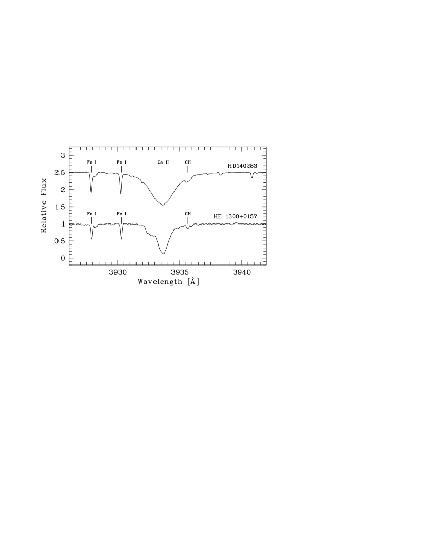
Figure 1.— Region around the Ca II K line in HE 1300+0157 and HD 140283 ($\mbox{[Fe/H]}\sim-2.5$). Some absorption features have been indicated.

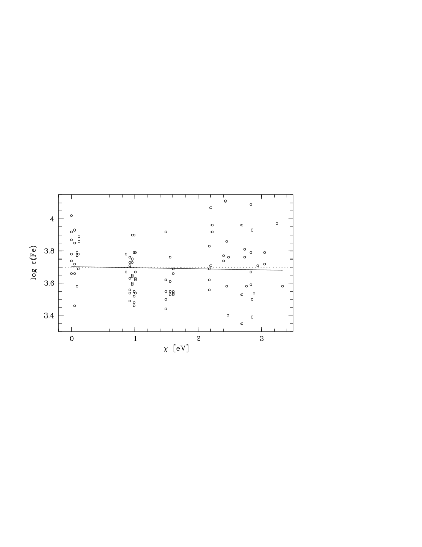
Figure 2.— LTE abundances $\log\epsilon(\rm Fe)$ of all measured Fe I lines as a function of excitation potential $\chi$ for the adopted subgiant stellar parameters. There is no significant trend of abundance found with $\chi$, indicating that the photometrically derived temperature is close to the value inferred from the excitation balance.

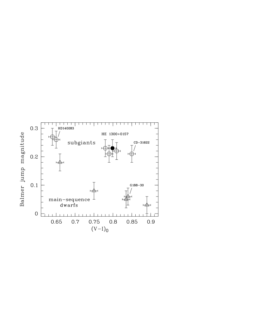
Figure 3.— Balmer jump magnitude as a function of $(V-I)_{0}$. Open circles indicate subgiants, whereas triangles indicate dwarf stars. HE 1300+0157 is shown with a filled circle.

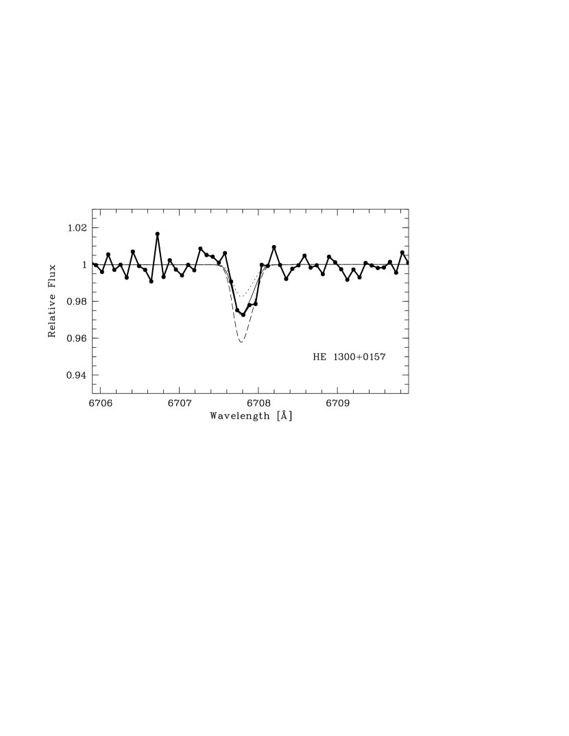
Figure 4.— Spectral region of the Li I doublet. The observed spectrum is shown (connected dots). Synthetic spectra with abundances of $A(\rm Li)=0.9$ (dotted line), $1.1$ (thin line) and $1.3$ (dashed line) are overplotted.

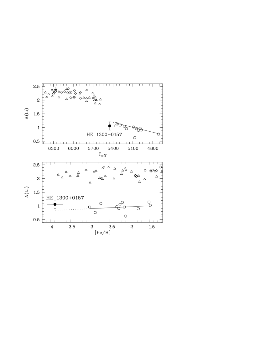
Figure 5.— Lithium abundances $A(\rm Li)$ for a sample of subgiants (open circles; García Pérez & Primas 2006) and selected main-sequence stars (triangles; Ryan et al. 1996a and diamonds; Ryan et al. 2001) as a function of effective temperature (top panel) and metallicity [Fe/H] (bottom panel). HE 1300+0157 is indicated with a filled circle.

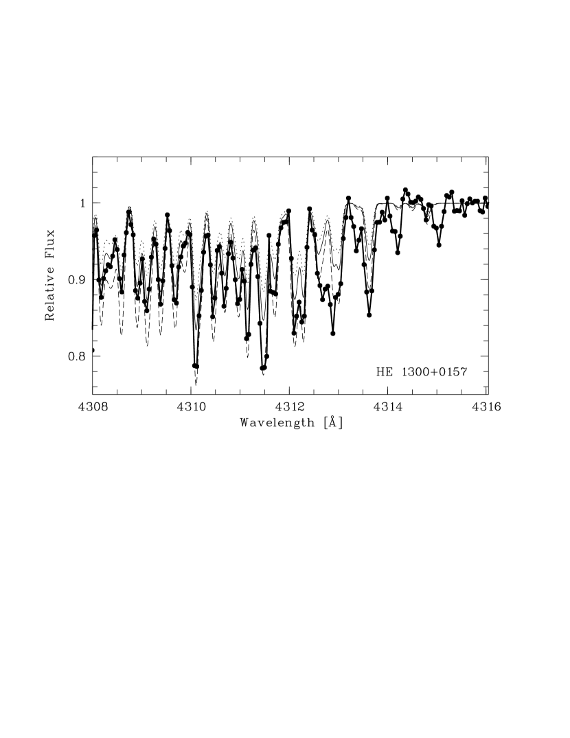
Figure 6.— Spectral region of the G-band band head at 4313 Å. The observed spectrum is shown (thin line). Synthetic spectra with abundances of $\mbox{[C/Fe]}=1.11$ (dotted line), $1.31$ (thin line), and $1.51$ (dashed line) are overplotted.

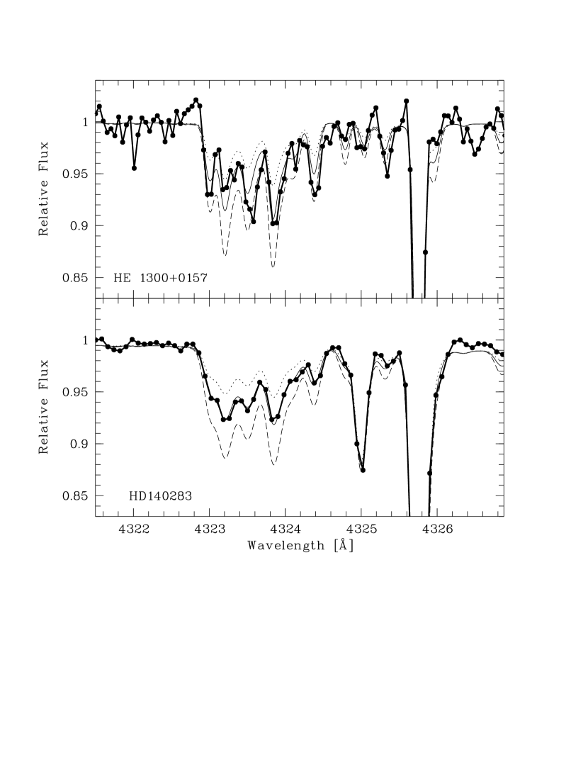
Figure 7.— Spectral region of the CH feature at 4323 Å for HE 1300$+$0157 (upper panel) and HD 140283 (lower panel). The observed spectrum is shown (thick line). For HE 1300$+$0157, synthetic spectra with abundances of $\mbox{[C/Fe]}=1.15$ (dotted line), $1.35$ (thin line), and $1.55$ (dashed line) are overplotted. For HD 140283, abundances of $\mbox{[C/Fe]}=0.34$ (dotted line), $0.54$ (thin line), and $0.74$ (dashed line) are shown.

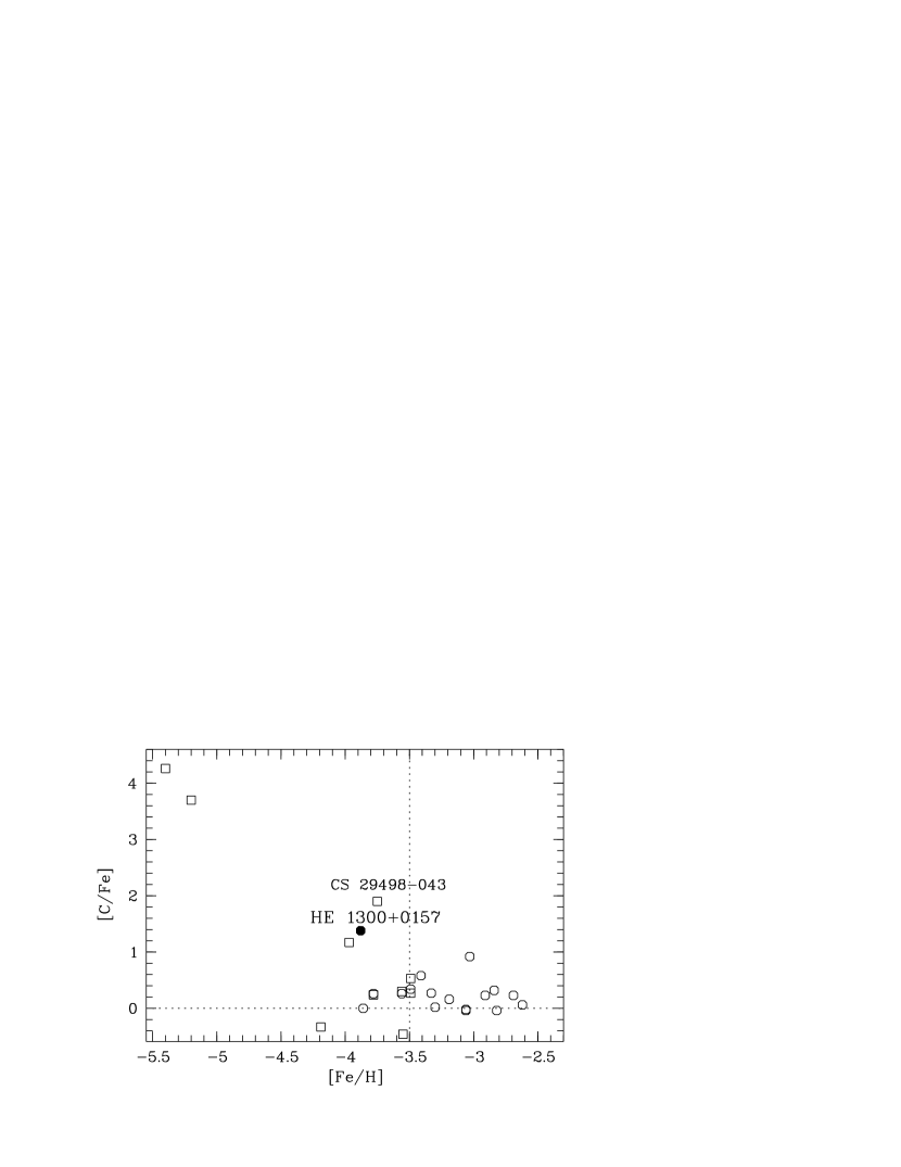
Figure 8.— 1D LTE carbon abundance ratios as a function of metallicity [Fe/H] of HE 1300+0157 (filled circle) and the unmixed stars of Spite et al. (2005, 2006) (open circles). The open squares refer to other stars with $\mbox{[Fe/H]}\lesssim-3.5$ (McWilliam et al. 1995; Aoki et al. 2002a; Cayrel et al. 2004 [mixed stars]; Cohen et al. 2004; Christlieb et al. 2004b; Aoki et al. 2006b)

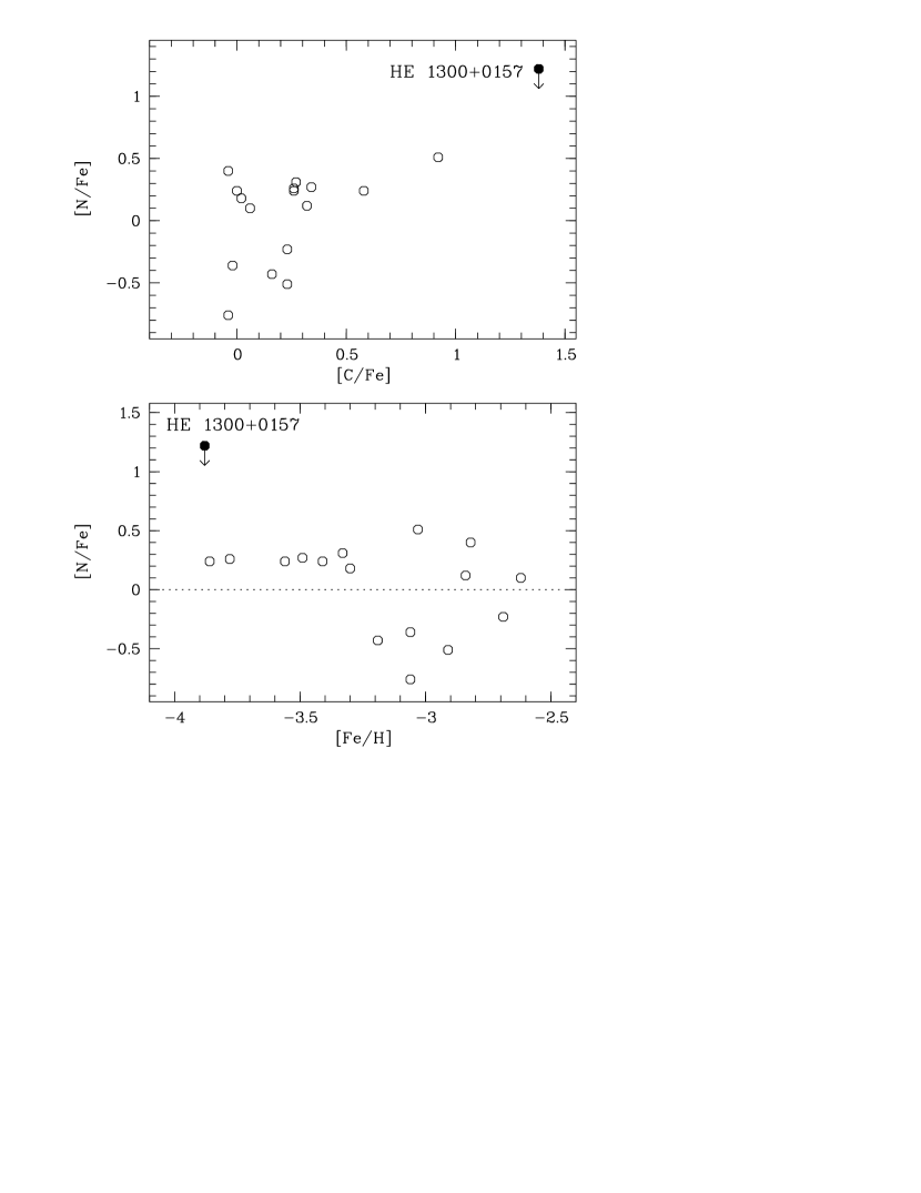
Figure 9.— 1D LTE nitrogen abundance ratio as a function of [C/Fe] (top panel) and [Fe/H] (bottom panel). The upper limit (arrow) for HE 1300$+$0157 is indicated with a filled circle. The open circles refer to the unmixed giants of Spite et al. (2005).

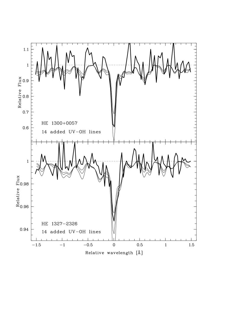
Figure 10.— Composite observed spectra (thick lines) consisting of 14 UV-OH lines for HE 1300$+$0157 (top panel) and HE 1327$-$2326 (bottom panel). For HE 1300$+$0157, synthetic spectra (thin lines) with abundances of $\mbox{[O/Fe]}=1.56$, 1.76, and 1.96 are overplotted. For HE 1327$-$2326, abundances of $\mbox{[O/Fe]}=3.48$, 3.68 and 3.88 are shown (Frebel et al. 2006a).

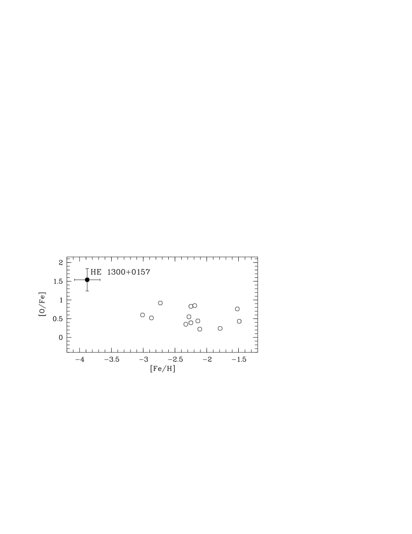
Figure 11.— Oxygen abundances [O/Fe] for a sample of subgiants as a function of metallicity [Fe/H]. The open circles refer to data taken from García Pérez et al. (2006), while HE 1300+0157 is marked with a filled circle. All abundance are determined from OH features. See text for discussion.

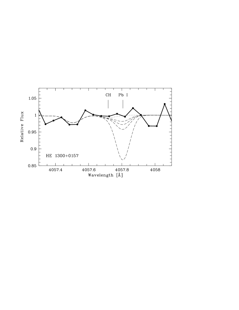
Figure 12.— Spectral region of the Pb I line. The observed spectrum is shown (connected dots). Synthetic spectra with abundances of $\mbox{[Pb/H]}=-1.5,-1.3-,1.1$, and $-0.5$ are overplotted (dashed lines). The dotted line refers to a synthetic spectrum where Pb is not included. Our upper limit is $\mbox{[Pb/H]}<-1.1$.

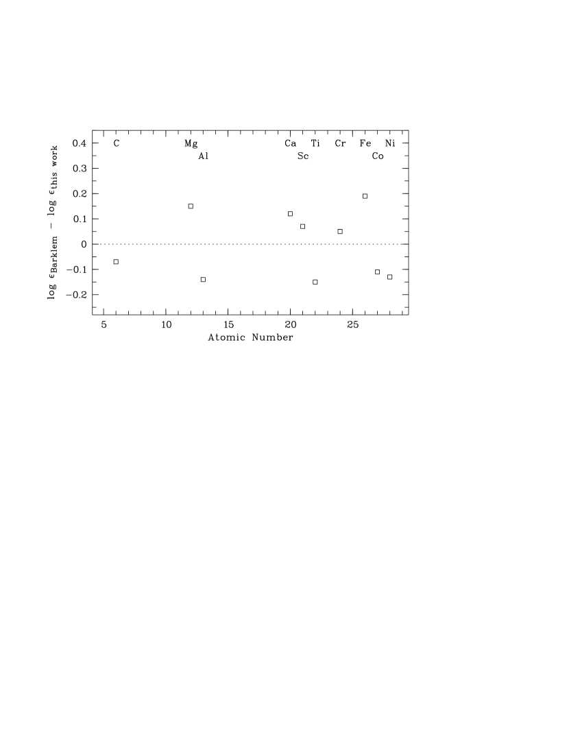
Figure 13.— Comparison of the abundances of Barklem et al. (2005) with the present study.

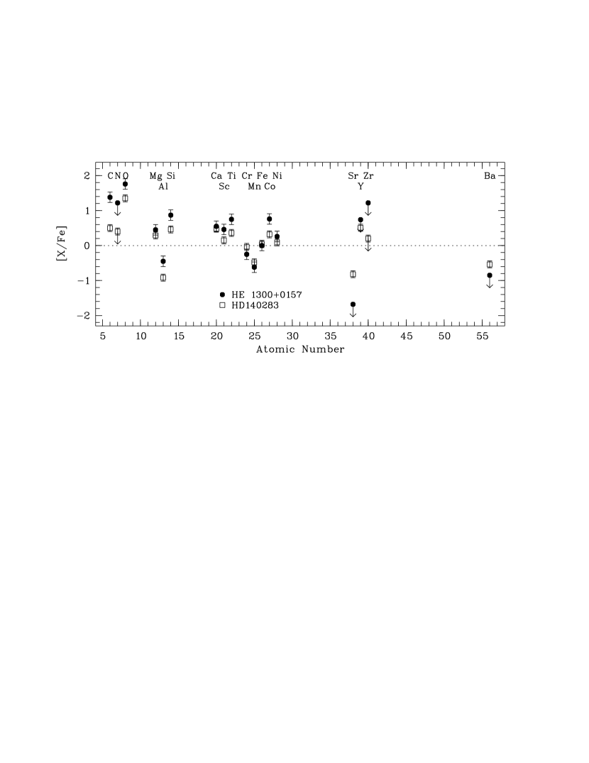
Figure 14.— LTE abundance pattern of HE 1300+0157 in comparison with that of HD 140283 (Ryan et al. 1996b; Boesgaard et al. 1999). The solar abundances of Asplund et al. (2005) have been employed for both sets of abundances.

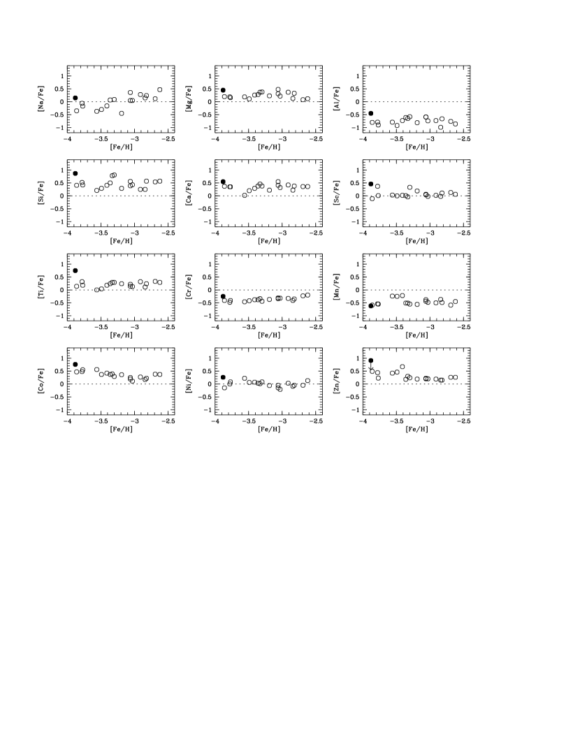
Figure 15.— 1D LTE abundances $\log\epsilon$ versus [Fe/H] for elements whose abundances were measured in HE 1300+0157 (filled circle) and 18 “unmixed” stars (open circles; Cayrel et al. 2004; Spite et al. 2006). See text for discussion.

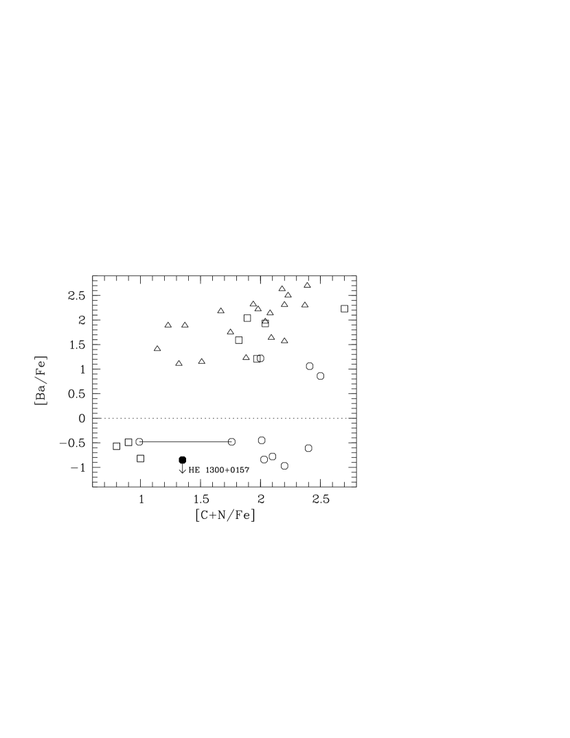
Figure 16.— Ba abundance ratio as a function of [C+N/Fe]. Open symbols refer to stars with $\mbox{[C/Fe]}>1.0$ and are taken from Norris et al. (1997, 2001), Aoki et al. (2002a, c, 2006a) and Cohen et al. (2006). Circles indicate stars with $\mbox{[Fe/H]}\leq-3.0$, squares indicate $-3.0<\mbox{[Fe/H]}\leq-2.7$ and triangles denote $\mbox{[Fe/H]}>-2.7$. HE 1300+0157 is indicated with a filled circle. See text for discussion.

References

- Alonso et al. (1996) Alonso, A., Arribas, S., & Martinez-Roger, C. 1996, A&A, 313, 873
- Anthony-Twarog & Twarog (1994) Anthony-Twarog, B. J. & Twarog, B. A. 1994, AJ, 107, 1577
- Aoki et al. (2005) Aoki, W., Beers, T. C., Christlieb, N., Frebel, A., Norris, J. E., Honda, S., Takada-Hidai, M., Asplund, M., Ando, H., Ryan, S. G., Tsangarides, S., Nomoto, K., Fujimoto, M. Y., Kajino, T., & Yoshii, Y. 2005, in IAU Symposium 228, ed. V. Hill, P. François, & F. Primas (Cambridge: Cambridge University Press), 195
- Aoki et al. (2006a) Aoki, W., Beers, T. C., Christlieb, N., Norris, J. E., Ryan, S. G., & Tsangarides, S. 2006a, ApJ, submitted
- Aoki et al. (2006b) Aoki, W., Frebel, A., Christlieb, N., Norris, J. E., Beers, T. C., Minezaki, T., Barklem, P. S., Honda, S., Takada-Hidai, M., Asplund, M., Ryan, S. G., Tsangarides, S., Eriksson, K., Steinhauer, A., Deliyannis, C. P., Nomoto, K., Fujimoto, M. Y., Ando, H., Yoshii, Y., & Kajino, T. 2006b, ApJ, 639, 897
- Aoki et al. (2006c) Aoki, W., Honda, S., Beers, T. C., Takada-Hidai, M., Iwamoto, N., Tominaga, N., Umeda, H., Nomoto, K., Norris, J. E., & Ryan, S. G. 2006c, ApJ, submitted
- Aoki et al. (2002a) Aoki, W., Norris, J. E., Ryan, S. G., Beers, T. C., & Ando, H. 2002a, ApJ, 576, L141
- Aoki et al. (2002b) —. 2002b, PASJ, 54, 933
- Aoki et al. (2002c) —. 2002c, ApJ, 567, 1166
- Aoki et al. (2002d) Aoki, W., Ryan, S. G., Norris, J. E., Beers, T. C., Ando, H., & Tsangarides, S. 2002d, ApJ, 580, 1149
- Arpigny & Magain (1983) Arpigny, C. & Magain, P. 1983, A&A, 127, L7
- Asplund (2005) Asplund, M. 2005, ARA&A, 43, 481
- Asplund & García Pérez (2001) Asplund, M. & García Pérez, A. E. 2001, A&A, 372, 601
- Asplund et al. (2005) Asplund, M., Grevesse, N., & Sauval, A. J. 2005, in ASP Conf. Ser. 336: Cosmic Abundances as Records of Stellar Evolution and Nucleosynthesis, 25
- Barklem et al. (2005) Barklem, P. S., Christlieb, N., Beers, T. C., Hill, V., Bessell, M. S., Holmberg, J., Marsteller, B., Rossi, S., Zickgraf, F.-J., & Reimers, D. 2005, A&A, 439, 129
- Beers (1999) Beers, T. C. 1999, in ASP Conf. Ser. 165: The Third Stromlo Symposium: The Galactic Halo, ed. B. K. Gibson, R. S. Axelrod, & M. E. Putman, 202
- Beers & Christlieb (2005) Beers, T. C. & Christlieb, N. 2005, ARA&A, 43, 531
- Beers et al. (2006) Beers, T. C., Flynn, C., Rossi, S., Sommer-Larsen, J., Wilhelm, R., Marsteller, M., Lee, Y. S., De Lee, N., Krugler, J., Deliyannis, C. P., Zickgraf, F.-J., Holmberg, J., Onehag, A., Eriksson, A., Terndrup, D. M., Salim, S., Christlieb, N., & Frebel, A. 2006, ApJS, submitted
- Bessell (1979) Bessell, M. S. 1979, PASP, 91, 589
- Bessell (1983) —. 1983, PASP, 95, 480
- Bessell & Brett (1988) Bessell, M. S. & Brett, J. M. 1988, PASP, 100, 1134
- Boesgaard et al. (1999) Boesgaard, A. M., King, J. R., Deliyannis, C. P., & Vogt, S. S. 1999, AJ, 117, 492
- Bromm & Loeb (2003) Bromm, V. & Loeb, A. 2003, Nature, 425, 812
- Busso et al. (1999) Busso, M., Gallino, R., & Wasserburg, G. J. 1999, ARA&A, 37, 239
- Carney & Peterson (1981) Carney, B. W. & Peterson, R. C. 1981, ApJ, 245, 238
- Cayrel et al. (2004) Cayrel, R., Depagne, E., Spite, M., Hill, V., Spite, F., François, P., Plez, B., Beers, T., Primas, F., Andersen, J., Barbuy, B., Bonifacio, P., Molaro, P., & Nordström, B. 2004, A&A, 416, 1117
- Chiappini et al. (1999) Chiappini, C., Matteucci, F., Beers, T. C., & Nomoto, K. 1999, ApJ, 515, 226
- Christlieb (2003) Christlieb, N. 2003, Rev. Mod. Astron., 16, 191
- Christlieb et al. (2004a) Christlieb, N., Beers, T. C., Barklem, P. S., Bessell, M., Hill, V., Holmberg, J., Korn, A. J., Marsteller, B., Mashonkina, L., Qian, Y.-Z., Rossi, S., Wasserburg, G. J., Zickgraf, F.-J., Kratz, K.-L., Nordström, B., Pfeiffer, B., Rhee, J., & Ryan, S. G. 2004a, A&A, 428, 1027
- Christlieb et al. (2004b) Christlieb, N., Gustafsson, B., Korn, A. J., Barklem, P. S., Beers, T. C., Bessell, M. S., Karlsson, T., & Mizuno-Wiedner, M. 2004b, ApJ, 603, 708
- Cohen et al. (2004) Cohen, J. G., Christlieb, N., McWilliam, A., Shectman, S., Thompson, I., Wasserburg, G. J., Ivans, I., Dehn, M., Karlsson, T., & Melendez, J. 2004, ApJ, 612, 1107
- Cohen et al. (2006) Cohen, J. G., McWilliam, A., Shectman, S., Thompson, I., Christlieb, N., Melendez, J., Ramirez, S., Swensson, A., & Zickgraf, F.-J. 2006, AJ, 132, 137
- Deliyannis et al. (1990) Deliyannis, C. P., Demarque, P., & Kawaler, S. D. 1990, ApJS, 73, 21
- Depagne et al. (2002) Depagne, E., Hill, V., Spite, M., Spite, F., Plez, B., Beers, T., Barbuy, B., Cayrel, R., Andersen, J., Bonifacio, P., François, P., Nordström, B., & Primas, F. 2002, A&A, 390, 187
- Eggen (1990) Eggen, O. J. 1990, AJ, 100, 1159
- François et al. (2003) François, P., Depagne, E., Hill, V., Spite, M., Spite, F., Plez, B., Beers, T. C., Barbuy, B., Cayrel, R., Andersen, J., Bonifacio, P., Molaro, P., Nordström, B., & Primas, F. 2003, A&A, 403, 1105
- Frebel et al. (2005) Frebel, A., Aoki, W., Christlieb, N., Ando, H., Asplund, M., Barklem, P. S., Beers, T. C., Eriksson, K., Fechner, C., Fujimoto, M. Y., Honda, S., Kajino, T., Minezaki, T., Nomoto, K., Norris, J. E., Ryan, S. G., Takada-Hidai, M., Tsangarides, S., & Yoshii, Y. 2005, Nature, 434, 871
- Frebel et al. (2006a) Frebel, A., Christlieb, N., Norris, J. E., Aoki, W., & Asplund, M. 2006a, ApJ, 638, L17
- Frebel et al. (2006b) Frebel, A., Christlieb, N., Norris, J. E., Beers, T. C., Bessell, M. S., Rhee, J., Fechner, C. Marsteller, M., Rossi, S., Thom, C., Wisotzki, L., & Reimers, D. 2006b, astro-ph/0608332
- Fryer et al. (2001) Fryer, C. L., Woosley, S. E., & Heger, A. 2001, ApJ, 550, 372
- Gallino et al. (1998) Gallino, R., Arlandini, C., Busso, M., Lugaro, M., Travaglio, C., Straniero, O., Chieffi, A., & Limongi, M. 1998, ApJ, 497, 388
- García Pérez et al. (2006) García Pérez, A. E., Asplund, M., Primas, F., Nissen, P. E., & Gustafsson, B. 2006, A&A, 451, 621