Testing Gaussianity on Archeops Data

Abstract

Aims. A Gaussianity analysis using a goodness-of-fit test and the Minkowski functionals on the sphere has been performed to study the measured Archeops Cosmic Microwave Background (CMB) temperature anisotropy data for a 143 GHz Archeops bolometer. We consider large angular scales, greater than 1.8 degrees, and a large fraction of the North Galactic hemisphere, around 16%, with a galactic latitude $b>15$ degrees.

Methods. The considered goodness-of-fit test, first proposed by Rayner & Best (1989), has been applied to the data after a signal-to-noise decomposition. The three Minkowski functionals on the sphere have been used to construct a $\chi^{2}$ statistic using different thresholds. The first method has been calibrated using simulations of Archeops data containing the CMB signal and instrumental noise in order to check its asymptotic convergence. Two kind of maps produced with two different map-making techniques (coaddition and Mirage) have been analysed.

Results. Archeops maps for both Mirage and coaddition map-making, have been found to be compatible with Gaussianity. From these results we can exclude a dust and atmospheric contamination larger than 7.8% (90% CL). Also the non-linear coupling parameter $f_{nl}$ can be constrained to be $f_{nl}=200_{\leavevmode\nobreak\ -800}^{\leavevmode\nobreak\ +1100}$ at the 95% CL and on angular scales of 1.8 degrees. For comparison, the same method has been applied to data from the NASA WMAP satellite in the same region of sky. The 1-year and 3-year releases have been used. Results are compatible with those obtained with Archeops, implying in particular an upper limit for $f_{nl}$ on degree angular scales.

1 Introduction

According to the inflationary universe theory (see for example Guth, 1981; Linde, 1990; Lyth & Riotto, 1998; Liddle & Lyth, 2000), the primordial density fluctuations are distributed following very precisely a Gaussian probability density function (pdf). These fluctuations in the matter density will produce anisotropies in the temperature of the Cosmic Microwave Background (CMB) whose pdf is also Gaussian. In this manner, when the Gaussianity of the CMB radiation is analysed the standard inflationary theory is tested as well as its alternatives (for example cosmic strings) which generically predict deviations from it in different ways. In addition, the search for non-Gaussianities has become a powerful tool to detect the presence of residual foregrounds, secondary anisotropies (such as gravitational lensing, Sunyaev-Zel’dovich effect) and unidentified systematic errors, which leave clearly non-Gaussian imprints on the CMB-anisotropies data. There are many techniques to test Gaussianity, many of them developed previously as general statistical methods to test the normality of a data set, and others specifically for the CMB anisotropies.

Among those methods, we can mention the estimator for non-Gaussianity based on the CMB bispectrum (Ferreira et al., 1998; Magueijo, 2000), geometrical estimators on the sphere (Barreiro et al., 2001; Monteserín et al., 2005, 2006) Minkowski functionals (Gott et al., 1990; Komatsu et al., 2003), goodness-of-fit tests (Rayner & Best, 1989; Aliaga et al., 2003; Barreiro et al., 2006), wavelets (Ferreira et al., 1997; Hobson et al., 1999; Barreiro et al., 2000) and steerable filters to search alignment structures (Wiaux et al., 2005).

Some of them have been applied to the CMB providing different results. For example WMAP data are compatible with Gaussianity according to the WMAP team (see Komatsu et al., 2003; Spergel et al., 2007) whereas others have found evidences of non-Gausssianities in the same WMAP maps, like Copi et al. (2004, 2006) (using a technique called multipole vector framework), Eriksen et al. (2004, 2005) (finding asymmetries using local estimators of the n-point correlations), Vielva et al. (2004); Cruz et al. (2005, 2006, 2007) (the Cold Spot detected with wavelets), Larson et al. (2004) (cold and hot spots different from the ones expected in Gaussian temperature fluctuations), among others.

In this work the smooth goodness-of-fit test first proposed by Rayner & Best (1989) (hereafter R&BT) will be implemented to analyse the Gaussianity of the Archeops data. This method has been already applied successfully to the MAXIMA (Cayón et al., 2003b) and VSA experiments (Aliaga et al., 2005; Rubiño-Martín et al., 2006). The Archeops data will be as well analysed with the morphological descriptors known as Minkowski functionals (Schmalzing & Górski, 1998; Gott et al., 1990). The idea is to use both methods in the Gaussianity analysis for comparison of the sensitivities of the two techniques and cross-checking of the results on the amount of dust contamination and the amplitude of the non-linear coupling parameter.

This is the first analysis of Gaussianity of the Archeops experiment data. We have analysed the data for one of the Archeops bolometer at 143 GHz. This bolometer is the most sensitive and one of the most relevant for CMB observations. As a complementary analysis, we present the results of the same goodness-of-fit test applied to WMAP data with approximately the same mask as the one used for Archeops. The purpose is to check whether the results are consistent for both data sets.

This paper has the following layout: in Section 2 the R&BT applied to signal-to-noise eigenmodes and the Minkowski functionals are described. The experiment, main properties of data sets and masks are summarized in Section 3. Section 4 is dedicated to the calibration and checking of both methods with some “realistic” CMB anisotropy Gaussian simulations, where we know in advance the output of the techniques. Section 5 contains the Archeops data analysis as well as results. In Section 6 WMAP 1-year and 3-year data are analysed and compared with Archeops results. Finally in Section 7 the main conclusions are presented.

2 Goodness-of-fit tests and Minkowski functionals

In this section, on the one hand, we will describe briefly the “goodness-of-fit technique” applied to test the Gaussianity of a set of “signal-to-noise eigenmodes” derived from measurements of the CMB temperature anisotropies. On the other hand, we will explain the Gaussianity analysis based on the Minkowski functionals.

2.1 Smooth tests of goodness-of-fit

Given a set of $n$ random numbers, $\{y_{i}\}_{i=1}^{i=n}$, it is sometimes interesting to check whether they behave statistically according to one specific pdf, $f(y,\theta)$, that is, if the probability of finding a random number $y$ in an interval between $y_{0}$ and $y_{0}+\Delta y$, with $\Delta y\geq 0$, is given by $f(y_{0},\theta)\Delta y$. A scalar or vector variable $\theta$ is introduced, which allows us to move smoothly between different pdf’s in their corresponding space of normalized functions.

This statistical analysis consists in testing the null hypothesis, $H_{0}:\{\theta=0\}$ against the alternative hypothesis, $K:\{\theta\neq 0\}$.

Inside the family of smooth goodness-of-fit tests, we can consider an order k alternative pdf $g_{k}(y,\theta)$, characterized by a pdf of the form (see Rayner & Best, 1989, 1990)

$$g_{k}(y,\theta)=C(\theta)\exp\biggl{[}\sum_{i=1}^{k}\theta_{i}h_{i}(y)\biggr{]}f(y)$$ (1)

$\theta$ is a set of $k$ parameters to smoothly cover our space of pdf’s, $f(y)$ is the null hypothesis pdf (e. g. the Gaussian distribution), $h_{i}(y)$ form a complete set of orthonormal functions on $f(y)$ and $C(\theta)$ is a normalization constant.

The “score statistic” is used to evaluate the simple null hypothesis $H_{0}$. With this statistic one can estimate the statistical significance of $\theta$ through the “Maximum Likelihood Method”. Following the notation by Aliaga et al. (2003), the score statistic for this goodness-of-fit test is

$$S_{k}=\sum_{i=1}^{k}U_{i}^{2}\ \ ,$$ (2)

and the $U_{i}^{2}$ quantities are given by

$$U_{i}=\sum_{j=1}^{n}\frac{h_{i}(y_{j})}{\sqrt{n}}$$ (3)

In the case of a Gaussian pdf, $h_{i}(x)$ are the “normalized Hermite-Chebyshev polynomials”. If the null hypothesis is satisfied then the $U_{i}$ quantities have a statistically normal behaviour and therefore $U_{i}^{2}$ behave like a $\chi_{1}^{2}$ distribution

$$f(U_{i}^{2})=\frac{1}{\sqrt{2\pi U_{i}^{2}}}e^{-\frac{-U_{i}^{2}}{2}}$$ (4)

It is possible to write the $U_{i}^{2}$ statistical quantities in terms of the moments of order $k$ derived from the set of $n$ random numbers to be analysed, $\mu_{k}=1/n\sum_{j=1}^{n}y_{j}^{k}$, (see for example Aliaga et al., 2003, 2005).

In this work, the five first statistics $U_{i}^{2}$ have been used and can be related to the $k$-order moments in the following way,

$$U_{1}^{2} = n(\mu_{1})^{2}$$

$$U_{2}^{2} = \frac{n}{2}(\mu_{2}-1)^{2}$$

$$U_{3}^{2} = \frac{n}{6}(\mu_{3}-3\mu_{1})^{2}$$

$$U_{4}^{2} = \frac{n}{24}(\mu_{4}-6\mu_{2}+3)^{2}$$

$$U_{5}^{2} = \frac{n}{120}(\mu_{5}-10\mu_{3}+15\mu_{1})^{2}$$ (5)

The first few statistics are generally the most sensitive for most of the applications. In our case higher order $U_{i}^{2}$ statistics are dominated by errors (because of usual propagation of errors) and therefore are not very useful in practice. This will be described in detail in section 4.

2.2 Signal-to-noise eigenmode analysis

At this point, we have described the method that will be used to analyse a set of $n$ random numbers to test whether their pdf is the normal distribution or not.

The next step is to compute the set of numbers to be analysed. In our case they come from the so called “signal-to-noise eigenmodes”, firstly introduced in the CMB field by Bond (1995). Our observational data, (the fluctuation in the temperature of the incoming blackbody radiation measured for each direction $\@vec{n}$ in the sky, $\Delta T(\@vec{n})/T$), can be interpreted as originated from several sources: all the emissions coming from the sky (CMB signal, Galactic and extragalactic foregrounds and atmosphere) and the measured instrumental Gaussian noise (Macías-Pérez et al., 2007).

The total area observed by the experiment is usually divided in equal area pixels identified by their center direction $\@vec{n}$ and to which the measurements, $\Delta T(\@vec{n})/T$, are assigned. To obtain the “signal-to-noise eigenmodes”, we expand the pixel values of the map, $\Delta T(\@vec{n})/T$, into a linear combination in which the transformed instrumental noise (hereafter the noise) and the transformed theoretical CMB signal (hereafter the signal) do not have correlations.

For the signal-to-noise decomposition it is necessary to calculate signal and noise covariance matrices. The temperature covariance between two pixels $i$ and $j$ is given by

$$C_{ij}=\langle\Delta T_{i}\Delta T_{j}\rangle-\langle\Delta T_{i}\rangle\langle\Delta T_{j}\rangle\\$$ (6)

where the brackets $\langle\rangle$ represent the average over several realizations of temperature anisotropy maps. Thus we can construct the signal (noise) covariance matrices, $S$ ($N$), averaging on signal $\Delta T_{s}(\@vec{n})$ (noise $\Delta T_{n}(\@vec{n})$) realizations. Since the data represent temperature fluctuations around the mean then it is trivially satisfied that $\langle\Delta T_{s}(\@vec{n})\rangle=\langle\Delta T_{n}(\@vec{n})\rangle=0$. Therefore, $C_{ij}=\langle\Delta T_{i}\Delta T_{j}\rangle$, the correlation matrix.

Once we select a set of $n$ directions in the sky (pixels) and we construct $S$ and $N$ matrices, which have the same dimension $n$ and are symmetrical, we can compute the so called “signal-to-noise matrix” $A$

$$A=L_{N}^{-1}SL_{N}^{-t}$$ (7)

where $L_{N}$ is the Cholesky matrix of $N$, defined as $N\equiv L_{N}L_{N}^{t}$. $L_{N}$ can be obtained from the diagonalization of the $N$ matrix. Suppose $D_{N}$ is the diagonal matrix of eigenvalues of $N$, and $R_{N}$ a matrix of the eigenvectors of $N$, related by $R_{N}^{t}NR_{N}=D_{N}$. Then it is satisfied that $L_{N}=R_{N}D_{N}^{1/2}$, where $D_{N}^{1/2}$ is the square root matrix of $D_{N}$.

If $\@vec{d}$ is the vector of dimension $n$ representing the data assigned to the pixels in the sky, the signal-to-noise eigenmodes can be written as

$$\@vec{\xi}=R_{A}^{t}L_{N}^{-1}\@vec{d}$$ (8)

where $R_{A}$ is the matrix of eigenvectors of $A$ and $D_{A}$ the diagonal matrix of eigenvalues of $A$, $R_{A}^{t}AR_{A}=D_{A}$.

The ${y_{i}}$ quantities to be analysed with the goodness-of-fit test defined in the previous section are

$$y_{i}=\frac{\xi_{i}}{\sqrt{1+(D_{A})_{i}}}$$ (9)

It can be easily demonstrated that if the vector of data $\@vec{d}$ satisfies $\langle\@vec{d}\rangle=0$ then $\langle y_{i}\rangle=0$. In the case $\Delta T=\Delta T_{s}+\Delta T_{n}$, from the definition of signal-to-noise eigenmodes in (8), the definition of $y_{i}$ in (9), and properties of correlation matrices it follows that $\langle y_{i}^{2}\rangle=1$.

Supposing that the original map $\@vec{d}$ is multi-normal, then our $\{y_{i}\}$ numbers keep the Gaussian character because both set of numbers are connected by linear operations. More precisely, they follow a normal pdf with zero mean and unit variance, $N(0,1)$. Moreover, for different indexes $i$ and $j$, $y_{i}$ and $y_{j}$ are independent.

Finally, for Gaussian data $\@vec{d}$ each $U_{i}^{2}$ statistics, defined in (3), is distributed as a $\chi_{1}^{2}$. The decision to accept or reject the null hypothesis will be therefore based on this pdf, as will be seen in sections 5 and 6 when the test is applied to the Archeops and WMAP data.

2.3 Minkowski functionals

Considering the temperature anisotropies of the CMB as a scalar field on the sphere we can define the set of coordinates $Q_{\nu}$ where $\Delta T(\@vec{n})>\nu$ for a given threshold $\nu$, and its complementary set $V_{\nu}$. As it is stated in Schmalzing & Górski (1998), any morphological descriptor on the sphere is a linear combination of 3 Minkowski functionals. These functionals are: the area $A(\nu)$ of the excursion set $Q_{\nu}$, the contour length $C(\nu)$ of the excursion set $Q_{\nu}$, and the genus $G(\nu)$ (defined as the number of hot spots above $\nu$ minus the number of cold spots below that threshold).

For a Gaussian random field the mean values of these functionals are

$$\langle A(\nu)\rangle = \frac{1}{2}\left(1-\frac{2}{\sqrt{\pi}}\int_{0}^{\nu/2}exp(-t^{2})dt\right)$$

$$\langle C(\nu)\rangle = \frac{\sqrt{\tau}}{8}exp(-\frac{\nu^{2}}{2})$$

$$\langle G(\nu)\rangle = \frac{\tau}{(2\pi)^{3/2}}\leavevmode\nobreak\ \nu\leavevmode\nobreak\ exp(-\frac{\nu^{2}}{2})$$

where $\tau$ is a parameter related with the coherence angle (Barreiro et al., 2001; Schmalzing & Górski, 1998).

The Gaussianity test with the Minkowski functionals is performed through a $\chi^{2}$ test as described for example in Komatsu et al. (2003); Spergel et al. (2007). Considering $n_{th}$ possible thresholds $\nu$ we can define a $3n_{th}$ vector $\@vec{v}=(A(\nu),C(\nu),G(\nu))$. The $\chi^{2}$ statistic is then defined

$$\chi^{2}=\sum_{i,j}(\@vec{v}(i)-\langle\@vec{v}(i)\rangle)C^{-1}_{ij}(\@vec{v}(j)-\langle\@vec{v}(j)\rangle)$$ (11)

where $\langle\@vec{v}(j)\rangle$ is the expected value of $v(j)$ and $C$ is the corresponding covariance matrix for all possible thresholds and functionals.

3 Archeops data sets

3.1 The Archeops experiment

Archeops is a balloon borne experiment dedicated to measure the CMB temperature anisotropies from large to small angular scales (Benoît et al., 2003a; Tristram et al., 2005). It has given the first link in the $C_{\ell}$ determination between the COBE large angular scales data (Smoot et al., 1992) to the first acoustic peak as measured by BOOMERanG and MAXIMA (de Bernardis et al., 2000; Hanany et al., 2000). Archeops was also designed as a test bed for the forthcoming Planck High Frequency Instrument (HFI), (Lamarre et al., 2003). Therefore, Archeops shared with Planck the same technological design: a Gregorian off-axis telescope with a 1.5 m primary mirror, bolometers operating at 143, 217, 353 and 545 GHz cooled down at 100 mK by a ³He/⁴He dilution designed to work at zero gravity and a similar scanning strategy. Archeops was launched on February 7^th, 2002, from the CNES/Swedish facility of Esrange, near Kiruna (Sweden). 12 hours of high quality night data were gathered. This data corresponds to a coverage of approximately 30% of the sky, including the Galactic plane. More details about the instrument and the flight performance can be found in Benoît et al. (2003b); Macías-Pérez et al. (2007). From its four frequency bands the two lowest (143 and 217 GHz) were dedicated to the observation of the CMB and the others (353 and 545 GHz) to the monitoring and calibration of both atmospheric and Galactic emissions.

In the following, we focus on the analysis of the most sensitive 143 GHz Archeops bolometer that also presents the lowest level of contamination by systematic effects.

Although the Archeops resolution is typically of 10 arcmin, for this analysis we are interested in the Gaussianity of the large angular scale anisotropies. Therefore, we decided to use low resolution maps at HEALPix (Górski et al., 2005) $N_{\rm side}=32$ to consider scales above 1.8 degrees.

3.2 Data processing

We describe here briefly the way that Archeops data were processed. For a more detailed description see Macías-Pérez et al. (2007).

In the Time Ordered Information (TOI) corrupted data are flagged (representing less than 1.5% of the whole data set). Low frequency drifts, correlated to house-keeping data are removed using the latter as templates. A high frequency decorrelation is also performed to remove some bursts of non-stationary high-frequency noise. Corrected timelines are then deconvolved from the bolometer time constant and the flagged corrupted data are replaced by a realization of noise. Finally, low time frequency atmospheric residuals are subtracted using a destriping procedure which slightly filters out the sky signal to a maximum of 5%.

Archeops cleaned TOIs at 143 GHz are contaminated by atmospheric and Galactic dust residuals, even at intermediate Galactic latitudes. Atmospheric residuals contributes mainly at frequencies lower than 2 Hz in the timeline and follows approximatively a $\nu^{2}$ law in antenna temperature. Galactic dust presents a grey body spectrum at about 17 K and with an emissivity of about $\nu^{2}$. To suppress both residual dust and atmospheric signals, data are decorrelated using a linear combination of the high frequency photometric pixels (353 and 545 GHz) and of synthetic dust timelines.

We have used in this work two kind of map-making for the TOIs of Archeops data and of the simulations. The first one is an optimal map-making procedure called Mirage (Yvon & Mayet, 2005). Mirage is based on a two-phase iterative algorithm, involving optimal map-making together with low frequency drift removal and Butterworth high-pass filtering. A conjugate gradient method is used for resolving the linear system. The second is a procedure that performs coaddition. This means that all the TOI points corresponding to a given pixel are averaged.

To produce a CMB simulation, a random CMB map with the power spectrum of the Archeops model (see Benoît et al. (2003b) and figure 1) is generated and from this map an Archeops TOI is produced. This TOI is treated with the two map-making methods described above to produce a map. To perform a noise simulation we produce a Gaussian constrained realization of the Archeops noise power spectrum in the time domain. The TOI produced this way is then projected into a map using the above map-making techniques.

The analysis has been performed on a fraction of the Archeops observed region masking out pixels with Galactic latitude below 15 degrees, $|b|<15^{o}$. The southern sky data were not included in the analysis as they are more contaminated by systematics in the form of residual stripes coming from the Fourier filtering and destriping of the data in the time domain (Macías-Pérez et al., 2007) that produces ringing around the Galactic plane. In the case of the CMB power spectrum analysis presented in Tristram et al. (2005) this southern sky region was used as increased significantly the signal to noise ratio at small angular scales which are not affected by this systematic effect. This is not the case for the analysis presented in this paper where we are more interested in large angular scales where this systematic becomes important. In figure 2 we plot the region of data considered for the analysis. These data correspond to 1995 pixels (16% of the sky) from a total of 12288 pixels for a complete map at this resolution.

Figure 1: Archeops Best Fit Power Spectrum used to simulate the Archeops CMB signal.

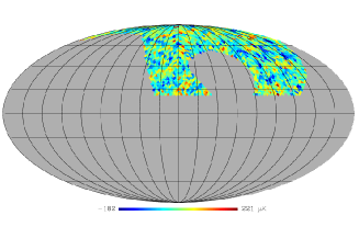
Figure 2: Mirage Archeops data from the best bolometer at 143 GHz presented at HEALPix resolution $N_{side}=32$, ($\approx 1.8$ degrees). This map is centered on Galactic longitude $l$ = 180 degrees. Galactic and South Equator pixels have been masked. Grid lines are spaced by 20 degrees.

4 Calibrating the method: analysis on Gaussian simulations

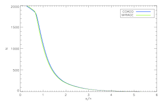
Figure 3: Number of normalized signal-to-noise eigenmodes $y_{i}$ for which their associated $A$ matrix eigenvalues, $(D_{A})_{i}$, satisfy $(D_{A})_{i}\geq(s/n)_{c}^{2}$.

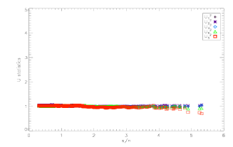
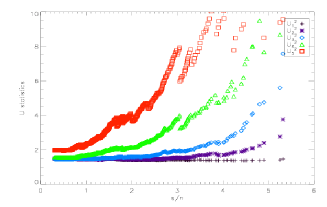
Figure 4: From left to right, mean and dispersion of $U_{i}^{2}$ statistics (where $i$ goes from 1 to 5) for different signal-to-noise cuts, corresponding to $10^{4}$ signal plus noise Mirage simulations.

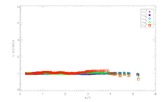
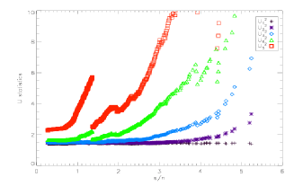
Figure 5: From left to right, mean and dispersion of $U_{i}^{2}$ statistics (where $i$ goes from 1 to 5) for different signal-to-noise cuts, corresponding to $10^{4}$ signal plus noise coaddition simulations.

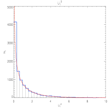
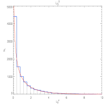
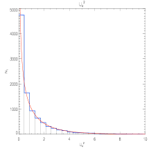
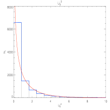
Figure 6: From left to right, and from top to bottom, distribution of the $U_{i}^{2}$ statistics, from a set of $10^{4}$ Gaussian Mirage simulations analysed in the same region than the data (figure 2). The signal-to-noise cut which has been used is $(s/n)_{c}=0.30$. Solid lines are the theoretical distribution ($\chi_{1}^{2}$) normalized to the number of simulations and the size of the binned cell.

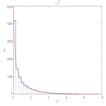
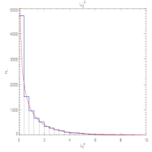
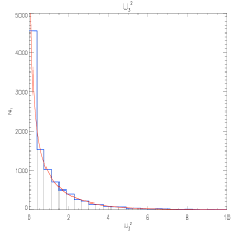
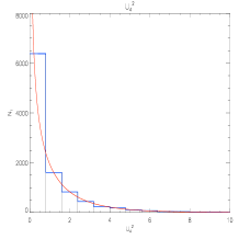
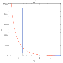
Figure 7: From left to right, and from top to bottom, distribution of the $U_{i}^{2}$ statistics, from a set of $10^{4}$ Gaussian coaddition simulations analysed in the same region than the data (figure 2). The signal-to-noise cut which has been used is $(s/n)_{c}=0.27$. Solid lines are the theoretical distribution ($\chi_{1}^{2}$) normalized to the number of simulations and the size of the binned cell.

Figure 8: From left to right, mean values of the three Minkowski functionals and their corresponding error-bars for a set of 1000 (noiseless) CMB Gaussian simulations. These simulations have been generated using Archeops best fit power spectrum and have not been masked. Notice the good agreement between the theoretical predictions and the results obtained from simulations.

To develop the R&BT non-Gaussianity test, it is necessary to calculate the signal (S) and the noise (N) correlation matrices among the selected pixels. We computed these matrices averaging on simulations by means of equation 6. For this purpose Monte Carlo Gaussian simulations of Archeops CMB signal and instrumental noise were produced. The number of performed simulations for the map generated with the Mirage map-making procedure were $2.86\times 10^{5}$ for the signal and $2.75\times 10^{5}$ for the noise, whereas for the coaddition procedure they were $5\times 10^{5}$ and $5\times 10^{5}$ for the signal and noise respectively. 90 dual-core 3.2 GHz processors from the IFCA computing facilities were used. Each Mirage simulation took 180 s of real CPU time and 1.0 GB of RAM memory, whereas these values were 70 s and 0.04 GB respectively for each coaddition simulation.

The high number of simulations and the corresponding computational requirements were needed to achieve convergence in the construction of the correlation matrices. The main reason for the low convergence relies on the specific properties of our correlation matrices. Archeops noise is correlated at large scales, which means that the $N$ matrix is neither diagonal nor sparse. The Archeops signal correlation matrix contains correlations at large scales for which the convergence is much slower than for the small scales due to the cosmic variance. In both cases many simulations ($\sim 10^{5}$) were required in order to compute these matrices.

One way to quantify the degree of convergence of these matrices is by analysing Gaussian simulations. The $U_{i}^{2}$ statistics for a set of Gaussian simulations should have a $\chi_{1}^{2}$ pdf. This can be tested, for example, by calculating the mean and the variance of the $U_{i}^{2}$ statistics for $10^{4}$ Gaussian signal plus noise simulations. For the Gaussian case, the mean should be equal to 1 and the dispersion equal to $\sqrt{2}$ (this is the null hypothesis, $H_{0}$).

Following Aliaga et al. (2005); Rubiño-Martín et al. (2006), the $U_{i}^{2}$ are computed for a subset of signal-to-noise eigenmodes which are those associated with eigenvalues of the signal-to-noise matrix $A$ satisfying $(D_{A})_{i}\geq(s/n)_{c}^{2}$, where $(s/n)_{c}$ is a given signal-to-noise ratio cut. In figure 3 the number of eigenmodes $\{y_{i}\}$’s, which obey $(D_{A})_{i}\geq(s/n)_{c}^{2}$, in terms of $s/n$ is plotted.

In figure 4 we show the mean and dispersion of the five first $U_{i}^{2}$ statistics for different signal-to-noise cuts corresponding to all possible eigenvalues of the $A$ matrix. The $U_{i}^{2}$ values come from a set of $10^{4}$ Gaussian Archeops signal plus noise Mirage simulations. It can be seen that for $(s/n)_{c}\mathrel{\raise 1.72218pt\hbox{\hbox to0.0pt{$<$\hss}\lower 5.16663pt\hbox{$\sim$}}}2$ mean values are close to $1$ and the dispersion close to $\sqrt{2}$ (except for the $U_{5}^{2}$ statistic whose dispersion is always larger than 2). As shown by e.g. Aliaga et al. (2005), the expected value of $U_{i}^{2}$ is equal to 1 independently of the number of $\{y_{i}\}$ used. This explains why we have got the mean of $U_{i}^{2}$ very close to $1$ for every signal-to-noise cut. The dispersion is equal to $\sqrt{2}$ asymptotically, when the number of $\{y_{i}\}$ used is high. In our case, this happens for low signal-to-noise cuts, when enough $\{y_{i}\}$’s are used to compute the statistics. In figure 5 the same quantities have been plotted for the $10^{4}$ Gaussian Archeops signal plus noise coaddition simulations. Similar conclusions can be derived in this case. Notice, however, that the results are closer to theoretical values when the analysis is performed using the Mirage maps. In this case the correlation matrices have converged with less simulations than in the coaddition case. This is one of the advantages of using Mirage simulations over the coaddition ones, although the production of a Mirage map requires more CPU time and RAM memory than a coaddition map.

Since the computation of high order $U_{i}^{2}$ statistics involve high powers of the eigenmodes, the convergence of their dispersion to the theoretical values at a given $(s/n)_{c}$ is slower than for the low order ones (as can be seen in the right panels of figures 4 and 5).

A more exhaustive check for the convergence of the $U_{i}^{2}$ statistics is done by comparing their theoretical pdf with the histograms obtained from the simulated data. Given a signal-to-noise ratio cut $(s/n)_{c}$ for the calculation of the $U_{i}^{2}$ statistics, it is possible to make a histogram with the corresponding values of the $U_{i}^{2}$ statistics from the same sets of $10^{4}$ simulations. Figure 6 compares the histograms for the first five statistics calculated using all the eigenmodes ($s/n\geq 0.30$) for the Mirage simulations with the theoretical expectation of a $\chi_{1}^{2}$ distribution. In table 2 the mean and the dispersion of these histograms are presented. In figure 7 the same comparison is shown for the coaddition simulations considering also all the eigenmodes ($s/n\geq 0.27$). The corresponding mean and dispersion of these histograms are given in table 2.

In summary, the four statistics $U_{1}^{2}$, $U_{2}^{2}$, $U_{3}^{2}$, and $U_{4}^{2}$ have a pdf’s compatible with the theoretical one whereas $U_{5}^{2}$ starts to deviate from it. The discrepancy, already present in the dispersion, increases for higher orders. The reason is that high order moments enlarge possible errors present in the computed correlation matrices and are propagated in the diagonalization processes. In any case, the $U_{5}^{2}$ statistic can still be used for the Gaussian analysis if the distribution obtained from the simulations, instead of the theoretical one, is used as reference. Although this is not as optimal as using the theoretical $\chi_{1}^{2}$ distribution, it is however a good compromise taking into account the huge computational resources needed to produce a very large number of simulations.

For the Minkowski functionals analysis the expected values given by equation 2.3 cannot be applied to our problem because of the contour restrictions of the mask and the presence of anisotropic noise. Nevertheless in order to test our Minkowski functional codes we performed an analysis on (noiseless) CMB Gaussian simulations over all sky and 1.8 degrees resolution generated using the best fit Archeops power spectrum. Analysing them for thresholds from $-2.5\sigma$ to $2.5\sigma$ (where $\sigma$ is the standard deviation of the corresponding simulation), we obtained that the results from simulations are compatible with the theoretical predictions (see fig. 8).

Table 1: Mean and dispersion of $U_{i}^{2}$ statistics from $10^{4}$ Mirage simulations for a signal-to-noise ratio cut of 0.30.

…	$U_{1}^{2}$	$U_{2}^{2}$	$U_{3}^{2}$	$U_{4}^{2}$	$U_{5}^{2}$	$\chi_{1}^{2}$
$\mu$	1.02	1.04	1.01	1.01	1.02	1.00
$\sigma$	1.45	1.47	1.43	1.55	1.96	1.41

Table 2: Mean and dispersion of $U_{i}^{2}$ statistics from $10^{4}$ coaddition simulations for a signal-to-noise ratio cut of 0.27.

…	$U_{1}^{2}$	$U_{2}^{2}$	$U_{3}^{2}$	$U_{4}^{2}$	$U_{5}^{2}$	$\chi_{1}^{2}$
$\mu$	0.99	1.02	1.02	1.02	1.00	1.00
$\sigma$	1.40	1.47	1.48	1.62	2.27	1.41

5 Gaussianity test on Archeops data

We have applied the R&BT to the Archeops $143K03$ bolometer map. The signal-to-noise eigenmodes have been computed with the correlation matrices described in section 4, for each map-making case. We have checked in that section that these signal and noise matrices provide $U_{i}^{2}$ statistics compatible with Gaussianity for Gaussian simulations.

We have applied this test to the Archeops data for the Mirage and coaddition map-making. The $U_{i}^{2}$ statistics, computed for the 1995 pixels of the previously described Archeops data, are displayed in figures 9 and 10. The $U^{2}_{i}$ statistics are plotted, from i = 1 to 5, versus the signal-to-noise eigenmode cut.

For the Mirage map-making, results are displayed on figure 9. We can see that all the $U_{i}^{2}$ statistics are below 5 for all the signal-to-noise cuts. This means that the data is compatible with Gaussianity.

For coaddition map-making, we can see from figure 10 that whatever the signal-to-noise eigenmode cut is, $U_{i}^{2}$ statistics for the 143K03 bolometer data are below 5, except for $U_{2}^{2}$ for signal-to-noise cuts below 0.5. It reaches the maximum value of 7.97 at the minimum signal-to-noise cut of 0.27. The upper tail probability for $U_{2}^{2}=7.97$ from the $\chi_{1}^{2}$ distribution (equation 4) is 0.5%. Comparing with the set of coaddition Gausian simulations we found that this upper tail probability is 0.6%, (see table 3), in good agreement with the theoretical expectation. Nevertheless, as we have computed $U_{i}^{2}$ statistics for all possible signal-to-noise cuts, it is important to estimate the significance of finding any simulation with $U_{2}^{2}\geq 7.97$ in at least one of them. This is the so called “p-value” of $U_{2}^{2}$. The “p-value” is defined as the probability that the relevant statistic takes a value at least as extreme as the one observed by the data when the null hypothesis is true. We have found for $U_{2}^{2}$ that the “p-value” is 15.0%.

Then we can conclude that even if we have a relatively strong $U_{2}^{2}$ at the lowest signal-to-noise ratio, it is not unlikely to have such a high value by chance. Therefore, even considering the results from the coaddition map-making, Archeops data is still compatible with our Gaussian simulations.

Although the high value found for $U_{2}^{2}$ for the coaddition map is not significant enough to be incompatible with Gaussianity, it is clear that there is a steady increase of $U_{2}^{2}$ when $s/n$ decreases. This suggests the presence of systematics in the coaddition maps that can depend on the resolution. Moreover, the fact that it only appears in coaddition data suggests the possibility that it is a map-making issue. This also implies that systematics are better controlled in the Mirage than in the coaddition map-making. Therefore hereafter we focus only on the Mirage map making data.

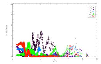
Figure 9: $U_{i}^{2}$ statistics of Mirage Archeops Data for different signal-to-noise cuts.

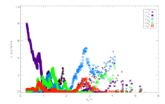
Figure 10: $U_{i}^{2}$ statistics of coaddition Archeops Data for different signal-to-noise cuts.

Table 3: $U_{i}^{2}$ from Archeops Mirage (coaddition) map for $(s/n)_{c}=0.30$ ($(s/n)_{c}=0.27$) and the probability that one $s+n$ Gaussian Mirage (coaddition) simulation has a $U_{i}^{2}$ statistic larger than those of data. More precisely, the probability for $U_{2}^{2}$ in the coaddition case is 0.6%.

…	$U_{1}^{2}$	$U_{2}^{2}$	$U_{3}^{2}$	$U_{4}^{2}$	$U_{5}^{2}$
Mirage	0.28	1.92	1.45	0.38	2.29
Prob.	0.60	0.17	0.23	0.54	0.12
Coaddition	0.11	7.97	0.10	0.04	0.34
Prob.	0.73	0.01	0.75	0.83	0.52

We performed a $\chi^{2}$ test with the three Minkowski functionals using 11 thresholds from $-2.5\sigma$ to $2.5\sigma$. We analysed the Mirage data and a set of 1000 CMB Gaussian simulations with noise of the Mirage type. The corresponding histogram of the $\chi^{2}$ values of these simulations and of the data are presented in figure 11. As it can be seen, the data are compatible with the Gaussian simulations.

Figure 11: Distribution of the $\chi^{2}$ values from the Minkonwski Gaussianity test for Archeops Mirage map. Vertical line shows the data results. Their cumulative probability is 83.9%.

5.1 Systematic and foreground contamination

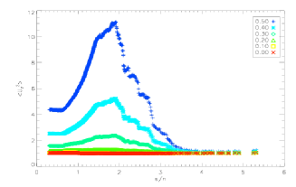
Figure 12: Mean of $10^{4}$ $U_{2}^{2}$ statistics, from $10^{4}$ signal plus noise Mirage simulations plus a factor $\alpha_{d}$ times the contamination template. $0.0\leq\alpha_{d}\leq 0.5$.

Figure 13: From left to right, $\chi^{2}$ value of Archeops data for different $\alpha_{d}$ and the histogram of best fit $\alpha_{d}$ for a set of 1000 Gaussian simulations without dust. These results have been obtained with the $U_{2}$ statistic.

The R&BT can also provide a powerful tool for estimating the level of this contribution. The test consists in adding different percentages of a template map to the Archeops 143K03 bolometer map, for the Mirage and coaddition simulations cases, to compare the resulting $U^{2}_{i}$ statistics to the ones obtained with the Archeops data at 143 GHz.

This template map is computed from the coadded Archeops 353 GHz map (see Ponthieu et al., 2005). This map contains thermal dust emission, atmospheric residuals as the dominant components and also instrumental noise and CMB residuals. Thus, extrapolated to 143 GHz it will provide a good template of what could be a dust plus atmospheric contamination at this frequency.

Thermal dust is assumed to have a grey-body emission: $\nu^{2}B(\nu)$ which can be approximated in the Rayleigh-Jeans domain to $T_{\rm RJ}\propto\nu^{2}$ (see Ponthieu et al., 2005). Atmospheric residuals emission law has been estimated empirically by the Archeops collaboration (see Macías-Pérez et al., 2007) and is also proportional to $\nu^{2}$ in the Rayleigh-Jeans domain. Dust and atmospheric residuals being the two main components, Archeops 353 GHz map has been extrapolated to 143 GHz by assuming that emission power law. Due to the extrapolation the CMB contribution on the 353 GHz template map is negligible with respect to the CMB at 143 GHz.

$U_{2}^{2}$ statistic is the most sensitive to this effect as can be seen in figure 12 for the Mirage case where this statistic presents a prominent peak at signal-to-noise ratio cuts around 1.88.

In order to determine the level of contamination we performed a $\chi^{2}$ test with the $U_{2}$ statistic computed at $(s/n)_{c}=1.88$. It is optimal to perform a $\chi^{2}$ test with $U_{2}$ because $U_{2}$ is normally distributed for the null hypothesis. Thus we can define

$$\chi^{2}(\alpha_{d})=\frac{1}{\sigma^{2}_{\alpha_{d}}(U_{2})}(U_{2}-\langle U_{2}\rangle_{\alpha_{d}})^{2}$$ (12)

where $\langle U_{2}\rangle_{\alpha_{d}}$ and $\sigma_{\alpha_{d}}(U_{2})$ are the mean and the dispersion of $U_{2}$ for CMB Gaussian simulations with noise plus a factor $\alpha_{d}$ times the contamination template. In the left panel of figure 13 we present the $\chi^{2}$ of Archeops Mirage data for different ${\alpha_{d}}$. We can see that the minimum $\chi^{2}$ (best fit) occurs for ${\alpha_{d}}$=0.0. Analysing Gaussian simulations without dust we find that most of them reach the best fit for low values of ${\alpha_{d}}$ (right panel of figure 13). Specifically we have that $\alpha_{d}\leq$ 0.27 for 90% confidence level (CL), and $\alpha_{d}\leq$ 0.33 for 95% CL. By comparing the dispersion of both maps, Archeops and 0.27 times the contamination template, we can exclude a dust plus atmospheric contamination larger than 7.8%.

We computed another $\chi^{2}$ statistic using the Minkowski functionals for the dust analysis. In this case

$$\chi^{2}(\alpha_{d})=\sum_{i,j}(\@vec{v}(i)-\langle\@vec{v}(i)\rangle_{\alpha_{d}})C^{-1}_{ij}(\@vec{v}(j)-\langle\@vec{v}(j)\rangle_{\alpha_{d}})$$ (13)

$i$ and $j$ cover 11 thresholds from $-2.5\sigma$ to $2.5\sigma$ and the three Minkowski functionals. $\langle\@vec{v}(i)\rangle_{\alpha_{d}}$ is the mean value of the corresponding functional at the corresponding threshold for Gaussian CMB simulations with noise plus $\alpha_{d}$ times the dust template. $C$ is the covariance matrix for Gaussian CMB simulations with noise. The value of $\alpha_{d}$ that best fits Archeops data is $\alpha_{d}=$ 0.0. Analysing Gaussian simulations without dust we find that $\alpha_{d}\leq$ 0.28 for 90% CL, and $\alpha_{d}\leq$ 0.35 for 95% CL.

5.2 Primordial non-Gaussianity

Figure 14: From left to right, $\chi^{2}$ value of Archeops data for different $f_{nl}$ and the histogram of best fit $f_{nl}$ for a set of 1000 CMB Gaussian simulations with noise. These results have been obtained with the Minkowski functionals.

There are several possible inflationary scenarios in which the primordial fluctuations are not Gaussian distributed. The idea is to work with a simple non-Gaussianity model and to impose some constraints on it. In particular, we consider the “weak non-linear coupling case” (Komatsu & Spergel, 2001; Liguori et al., 2003; Bartolo et al., 2004)

$$\Phi(\@vec{x})=\Phi_{L}(\@vec{x})+f_{nl}\{\Phi^{2}(\@vec{x})-\langle\Phi^{2}(\@vec{x})\rangle\}\ \$$ (14)

where $\Phi(\@vec{x})$ is the primordial gravitational potential, (which satisfies $\langle\Phi(\@vec{x})\rangle=0$), $\Phi_{L}(\@vec{x})$ is the linear random component (Gaussian distributed), and $f_{nl}$ is the non-linear dimensionless coupling parameter.

Scales larger than 1 degree are larger than the horizon scale at the recombination time, when CMB was formed (Liddle & Lyth, 2000). In this regime it is possible to make a good approximation linking CMB fluctuations and gravitational fluctuations through the Sachs-Wolfe effect (Sachs & Wolfe, 1967) $\Delta T(\@vec{n})/T=\Phi(\@vec{n})/3$ (notice however that a better approximation should include the integrated Sachs-Wolfe effect).

We analysed signal plus noise simulations with a $f_{nl}$ term in this way,

$$\Delta T^{\prime}_{s}(\@vec{n}) = \Delta T_{s}(\@vec{n})+\frac{3f_{nl}}{T}\{\Delta T_{s}(\@vec{n})^{2}-\langle\Delta T_{s}(\@vec{n})^{2}\rangle\}$$

$$\Delta T(\@vec{n}) = \Delta T^{\prime}_{s}(\@vec{n})+\Delta T_{n}(\@vec{n})\ \ ,$$ (15)

where $\Delta T_{s}$ is a Gaussian signal simulation, $\Delta T_{n}$ is a Gaussian noise simulation, $T=2.725\leavevmode\nobreak\ K$ and $\Delta T$ is the analysed simulation.

We performed a $\chi^{2}$ analysis for the primordial non-Gaussianity similar to the dust case for both $U_{2}$ and the Minkowski functionals. The signal-to-noise eigenmodes $y_{i}$ are weakly dependent on $f_{nl}$. It can be seen that the mean value of $y_{i}^{2}$ for simulations with $f_{nl}$ is

$$\langle y_{i}^{2}\rangle_{f_{nl}}=1+\frac{a_{i}}{1+(D_{A})_{i}}*f_{nl}+\frac{b_{i}}{1+(D_{A})_{i}}*f_{nl}^{2}$$ (16)

$$a_{i}=\frac{1}{T}\sum_{j,k}(R_{A}^{t}L_{N}^{-1})_{ij}(\langle s_{j}s_{k}^{2}\rangle+\langle s_{k}s_{j}^{2}\rangle)(L_{N}^{-t}R_{A})_{ki}$$ (17)

$$b_{i}=\frac{1}{T^{2}}\sum_{j,k}(R_{A}^{t}L_{N}^{-1})_{ij}(\langle s_{j}^{2}s_{k}^{2}\rangle+\langle s^{2}\rangle^{2})(L_{N}^{-t}R_{A})_{ki}$$ (18)

where $b_{i}$ is about an order of magnitude larger than $a_{i}$ for most of the $s/n$ eigenmodes. This implies that $\langle y_{i}^{2}\rangle_{f_{nl}}-1\sim O(f_{nl}^{2})$ which explains the low sensitivity of $U_{2}$ to $f_{nl}$ variations. In particular, we have found that it is much less sensitive than the Minkowski functionals. If we consider for example, a value of $f_{nl}=$ 2300, we find a relative variation $(\langle y_{i}^{2}\rangle_{f_{nl}}-\langle y_{i}^{2}\rangle_{0})/\langle y_{i}^{2}\rangle_{0}\simeq 0.05$ (and therefore a similar ratio for $U_{2}$ and $U_{2}^{2}$) for the former and $(\langle F^{2}\rangle_{f_{nl}}-\langle F^{2}\rangle_{0})/\langle F^{2}\rangle_{0}\simeq 0.50$ for the latter.

Therefore we performed a $\chi^{2}$ test with the three Minkowski functionals using different thresholds between $-2.5\sigma$ and $2.5\sigma$. In the left panel of figure 14 we present the $\chi^{2}$ value of the data for different $f_{nl}$ cases. We can see that the minimum $\chi^{2}$ value is reached for $f_{nl}=$ 200. Taking also into account the results obtained when analysing Gaussian simulations (see right panel of figure 14) we can put the following constraints on $f_{nl}$ from the Archeops data: $f_{nl}=200_{\leavevmode\nobreak\ -300}^{\leavevmode\nobreak\ +600}$ at 68% CL, $f_{nl}=200_{\leavevmode\nobreak\ -600}^{\leavevmode\nobreak\ +900}$ at 90% CL, and $f_{nl}=200_{\leavevmode\nobreak\ -800}^{\leavevmode\nobreak\ +1100}$ at 95% CL.

6 Complementary analysis: WMAP in the same region

WMAP is a NASA satellite dedicated to observe the anisotropies of the CMB with high accuracy at five different frequencies between 23 and 94 GHz. Scientific results of this mission have allowed us to have a clearer image of the early universe, and to reduce the uncertainties in several cosmological parameters. Data products of this mission can be found on the web.

6.1 The WMAP data

We have analysed WMAP data with the same goodness-of-fit and the Minkowski functionals tests already used on Archeops data. The main purpose of this analysis is to compare Archeops results with a different experiment to discriminate among systematics, foreground emissions and intrinsic CMB non-Gaussian features. It is clear that the WMAP frequencies complement very well the Archeops ones. A detailed analysis of the possible WMAP non-Gaussianities with this goodness-of-fit method deserves another work.

The maps that we have analysed have been produced from the 1-year and 3-year WMAP foreground cleaned maps for the differencing assemblies corresponding to the cosmological frequencies 40, 60 and 90 GHz. The main properties of these maps are described in detail in Bennett et al. (2003a); Hinshaw et al. (2007) respectively.

Specifically we have used the “combined map” as described in Bennett et al. (2003a), (see also Vielva et al., 2004). The WMAP CMB simulations which are used in the analysis are also combined simulations, that is, CMB signal simulations were produced for each channel and then combined in the same manner than for the data.

According to Bennett et al. (2003a) WMAP noise is highly uncorrelated, that is, the noise from a given pixel $i$ is independent of the noise from another pixel $j$. The noise combined simulations are produced from the “combined variance map” as it is shown in e.g. Vielva et al. (2004).

We have analysed both combined maps, 1-year and 3-year (hereafter WCM1 and WCM3). The WMAP mask considered for both analyses was the 3-year Kp0 one because it is the most conservative one for WCM3 and also contains the 1-year Kp0 mask. See Hinshaw et al. (2007) for details about new masks and Bennett et al. (2003b) for original masks. The actual mask we have used is the 3-year WMAP Kp0 degraded to our resolution times the Archeops mask. Its number of pixels is 1648. In figure 15 WCM3 data is plotted using this mask.

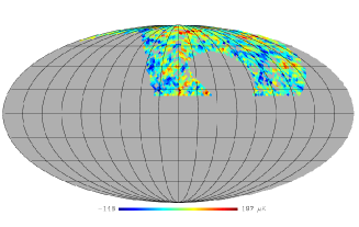
Figure 15: WCM3 Data at HEALPix resolution $N_{side}=32$ (it corresponds to a pixel size of $\approx 1.8$ degrees). This map is centered on Galactic longitude $l$ = 180 degrees. The pixels contaminated by Galactic and extragalactic emission are covered with the mask described in the text. Grid lines are spaced by 20 degrees.

6.2 Gaussianity test on WMAP data

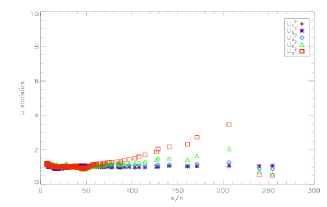
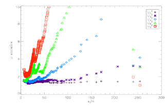
Figure 16: From left to right, mean and dispersion of $U_{i}^{2}$ statistics (where $i$ goes from 1 to 5) for different signal-to-noise cuts, corresponding to $10^{3}$ signal plus noise WCM3 simulations.

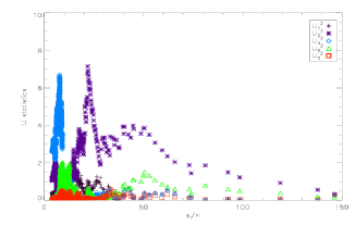
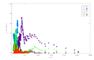
Figure 17: From left to right, $U_{i}^{2}$ statistics for WCM1 and WCM3 presented for different signal-to-noise cuts.

In order to perform the R&BT test on WCM1 and WCM3 maps we followed the same steps than for the Archeops analysis. We calculated their corresponding $S$ and $N$ matrices for the 1648 pixels available after applying the combined Archeops-WMAP mask.

We assume the best fit model of the 3-year WMAP data for both analysis, WCM1 and WCM3. At the resolution with which we are dealing, 1.8 degrees, the power spectra of the 1-year and 3-year data are very approximately the same. This assumption implies that the $S$ matrix is the same for both releases. The $S$ matrix is computed from $1.2\times 10^{5}$ Gaussian simulations following equation 6. Each simulation was produced in the same 90 dual core processors mentioned before, and took an average CPU time of 360 s and an average RAM memory of 0.4 GB.

As commented above, WMAP noise is highly uncorrelated and therefore we can assume that the noise matrices are diagonal. This means that the correlation element corresponding to pixels $i$ and $j$ is $N_{ij}=\sigma^{2}_{i}*\delta_{ij}$, where $\sigma^{2}_{i}$ is the combined noise of pixel $i$. Noise matrices for WCM1 and WCM3 must be constructed with their corresponding noise variances which differ by an approximate factor of 3.

Two additional sets of $10^{3}$ Gaussian signal plus noise simulations (corresponding to WCM1 and WCM3 maps) were performed for the calibration of the matrices. In figure 16, we present the mean and the dispersion of the $U_{i}^{2}$ statistics at different signal-to-noise cuts for the WCM3 case. Note that the numerical range for the possible signal-to-noise cuts $(s/n)_{c}$ is wider than for the Archeops case, because WCM3 noise is smaller than the Archeops one at this resolution. $(s/n)_{c}$ range for WCM1 is approximately the same than that of WCM3 reduced by a factor $\sqrt{3}$. The mean and the dispersion for WCM1 simulations are similar to those obtained for WCM3.

Table 4: Mean and dispersion of $U_{i}^{2}$ statistics from $10^{3}$ WCM1 simulations for $(s/n)_{c}=3.64$.

…	$U_{1}^{2}$	$U_{2}^{2}$	$U_{3}^{2}$	$U_{4}^{2}$	$U_{5}^{2}$	$\chi_{1}^{2}$
$\mu$	1.09	1.15	1.02	1.09	1.02	1.00
$\sigma$	1.56	1.50	1.47	1.71	2.02	1.41

Table 5: Mean and dispersion of $U_{i}^{2}$ statistics from $10^{3}$ WCM3 simulations for $(s/n)_{c}=6.33$.

…	$U_{1}^{2}$	$U_{2}^{2}$	$U_{3}^{2}$	$U_{4}^{2}$	$U_{5}^{2}$	$\chi_{1}^{2}$
$\mu$	1.00	1.18	1.04	1.10	1.22	1.00
$\sigma$	1.42	1.56	1.51	1.56	2.81	1.41

It can be seen that mean values of $U_{i}^{2}$ statistics are close to one for almost all signal-to-noise cuts and all the computed statistics, but the dispersion becomes higher than square root of two for high signal-to-noise cuts and for statistics with high order moments, like $U_{5}^{2}$ and higher order statistics.

As for the Archeops case, these high values are explained by the small errors present in the computed correlation matrices plus small numerical errors in the diagonalization of these matrices, which are amplified through the high order moments. In table 5 we present the mean and the dispersion of $U_{i}^{2}$ statistics for $10^{3}$ WCM1 simulations with noise for all the eigenmodes ($s/n\geq 3.64$). Note how the dispersion is increasing with the order of the statistics. In table 5 the same quantities are presented for $10^{3}$ WCM3, obtained also from all the eigenmodes ($s/n\geq 6.33$). The effect is the same for the high order moment statistics. The results for the $U_{i}^{2}$ statistics for WCM1 and WCM3 data maps are presented in figure 17. As can be seen, all $U_{i}^{2}$ values satisfy $U_{i}^{2}\leq 7.15$. The upper limit 7.15 corresponds to a upper tail probability of 0.7% for the theoretical distribution. In order to confirm or rule out a possible non-Gaussian detection, this result should be studied more carefully.

Figure 18: Distribution of the $\chi^{2}$ values from the Minkonwski Gaussian test for WCM3 data. Vertical line shows the data results. Their cumulative probability is 12.0%.

Table 6: WCM1 $U_{i}^{2}$ statistics for $(s/n)_{c}=21.81$, and their corresponding upper tail probabilities.

…	$U_{1}^{2}$	$U_{2}^{2}$	$U_{3}^{2}$	$U_{4}^{2}$	$U_{5}^{2}$
WCM1	0.90	7.15	0.32	0.63	0.09
Prob.	0.37	0.01	0.52	0.35	0.67

Table 7: WCM3 $U_{i}^{2}$ statistics for $(s/n)_{c}=37.92$, and their corresponding upper tail probabilities.

…	$U_{1}^{2}$	$U_{2}^{2}$	$U_{3}^{2}$	$U_{4}^{2}$	$U_{5}^{2}$
WCM3	0.13	7.15	0.00	0.61	0.01
Prob.	0.73	0.01	0.95	0.36	0.88

First of all, we have that for both WCM1 and WCM3 $U_{2}^{2}$ is the only statistic which reaches some sharp peaks above $6.6$ (which corresponds to a upper tail probability for the theoretical distribution of 1.0%). From the plots in figure 17, $U_{2}^{2}$ reaches this peak at $(s/n)_{c}=21.81$ for WCM1 and $(s/n)_{c}=37.92$ for WCM3. We estimated the upper tail probability for the $U_{i}^{2}$ statistics of data at the mentioned signal-to-noise cut by performing $10^{3}$ Gaussian simulations. These results are presented in tables 7 and 7. As we can see for the $U_{2}^{2}$ statistic, we have that this probability is 1.0% and 0.7% for WCM1 and WCM3 respectively, very similar to the theoretical value.

This probability is obtained for the precise signal-to-noise cut where $U_{2}^{2}$ reaches its maximum. Since the width of the maxima is much smaller than the range of variation of the signal-to-noise eigenvalues, it makes sense to ask for the significance of the detection. Thus, from the simulations we computed the “p-value”, i.e. the probability of finding a value of $U_{2}^{2}$ larger than 7.15 at any signal-to-noise cut, the maximum value reached by the data. This probability is 18% for WCM1 and 17% for WCM3.

From the previous discussion, we conclude that the sharp peaks found in the data are not significant. Also, well studied cases of artificial CMB non-Gaussianities, like skewness or kurtosis produced using the Edgeworth expansion (see Martínez-González E. et al. (2002) for applications of this expansion to the CMB non-Gaussianity analyses), usually show deviations of the $U_{i}^{2}$ statistics in the form of a large plateau. Besides, we would like to remark that at the signal-to-noise cuts where the maxima are found there are less than one hundred $\{y_{i}\}$ numbers to compute the $U_{i}^{2}$ statistics (around 70), and the test works correctly only asymptotically ($n>>1$).

WCM3 data were also analysed with the Minkowski functionals as in the Archeops case (that is, using 11 thresholds between $-2.5\sigma$ and $2.5\sigma$ and the three functionals). The histogram corresponding to the $\chi^{2}$ values for 1000 Gaussian simulations and the value for WCM3 data are presented in the figure 18. As we can see the WCM3 data are again compatible with Gaussianity.

Finally, we performed an analysis on simulations with $f_{nl}$ parameter as defined in equation 15. The procedure was the same as the one performed for Archeops case. As discussed in section 5.2, we only use the Minkowski functionals for the $f_{nl}$ case. The $\chi^{2}$ value for WCM3 data is minimum for $f_{nl}$ = 100. Analysing Gaussian simulations, the constraints found for $f_{nl}$ are: $f_{nl}=100_{\leavevmode\nobreak\ -200}^{\leavevmode\nobreak\ +200}$ at 68% CL, $f_{nl}=100_{\leavevmode\nobreak\ -300}^{\leavevmode\nobreak\ +400}$ at 90% CL, $f_{nl}=100_{\leavevmode\nobreak\ -400}^{\leavevmode\nobreak\ +500}$ at 95% CL. These limits are compatible with those obtained from Archeops since the tighter constraints found for WCM3 can be explained by the significantly smaller noise in that experiment. In particular, if we analyse simulated Archeops data with noise normalized to the same amplitude as that of WCM3 we find similar limits for $f_{nl}$.

7 Conclusions

The expected behaviour of the $U_{i}^{2}$ statistics as a $\chi_{1}^{2}$ distribution has been confirmed for the order index interval $1\leq i\leq 4$ with “realistic” simulations assuming Gaussian CMB anisotropies. For higher moments, $i>4$, the mean of the distribution is $\mu\simeq 1$ but the variance is $\sigma\mathrel{\raise 1.72218pt\hbox{\hbox to0.0pt{$>$\hss}\lower 5.16663pt\hbox{$\sim$}}}2$. This is because of the propagation of errors through higher order moments which in practice complicates the use of high order $U_{i}^{2}$ in our analysis.

From the analysis of both kind of Archeops maps, coaddition and Mirage, we have found that both are compatible with Gaussianity. Only the $U_{2}^{2}$ statistic for coaddition map is close to 8.0 for low $(s/n)_{c}$. Although in principle the probability that $U_{2}^{2}$ takes values bigger than 8.0 for a given signal-to-noise cut in the Gaussian hypothesis is very low (see table 3), the corresponding “p-value” for having $U_{2}^{2}$ larger than 8.0 at any signal-to-noise cut is 0.1482. This is not negligible and thus this detection is not significant. Moreover this effect does not appear in the Mirage map, and therefore should be assigned to issues related to the map-making process.

The analysis with the Minkowski functionals on the Mirage map also returns compatibility with Gaussianity.

Our analysis also implies constraints on the amount of contamination that can be present at 143 GHz. Using as template for dust and atmosphere the Archeops map at 353 GHz, we limit the possible contamination to be lower than 7.8% at 90% CL using $U_{2}$ statistic. A similar limit is obtained with the Minkowski functionals.

We have also compared the Archeops results with the WMAP 1 and 3-year data in the same region of the sky. For both sets of data a sharp peak in $U_{2}^{2}$ has been found at specific signal-to-noise cuts. Although the probability of finding such a peak at a given signal-to-noise cut is very small, the “p-value” obtained when different cuts are allowed is appreciable. Therefore we can conclude that the WMAP data, when the same region than Archeops is considered, are also consistent with Gaussianity. The same conclusion is reached when the data are analysed with the Minkowski functionals.

Finally, we have established a constraint in the value of the non-linear coupling parameter $f_{nl}$. Analysing Archeops data, we found that $f_{nl}=200_{\leavevmode\nobreak\ -600}^{\leavevmode\nobreak\ +900}$ at 90% CL, and $f_{nl}=200_{\leavevmode\nobreak\ -800}^{\leavevmode\nobreak\ +1100}$ at 95% CL. When the same analysis was done with WMC3 data using Archeops-WMAP combined mask, we found $f_{nl}=100_{\leavevmode\nobreak\ -300}^{\leavevmode\nobreak\ +400}$ at 90% CL, $f_{nl}=100_{\leavevmode\nobreak\ -400}^{\leavevmode\nobreak\ +500}$ at 95% CL. These limits are similar to the ones expected for an Archeops-like experiment with a noise amplitude similar to that of WCM3.