Stochastic excitation and damping of solar-type oscillations

Abstract

A review on acoustic mode damping and excitation in solar-type stars is presented. Current models for linear damping rates are discussed in the light of recent low-degree solar linewidth measurements with emphasis on the frequency-dependence of damping rates of low-order modes. Recent developments in stochastic excitation models are reviewed and tested against the latest high-quality data of solar-like oscillations, such as from alpha Cen A, and against results obtained from hydrodynamical simulations.

1 Introduction

Solar p modes are believed to be excited stochastically in the outer layers of the star by the turbulent convection. Accurate measurements are available from both space-borne (e.g., VIRGO, GOLF and MDI) and ground-based (GONG and BiSON) observations which provide valuable data regarding the excitation and damping processes influencing the modes. Such modes can be stochastically excited by the turbulent convection. The process can be regarded as multipole acoustical radiation (e.g. Unno 1964). For solar-like stars, the acoustic noise generated by convection in the star’s resonant cavity may be manifest as an ensemble of p modes over a wide band in frequency (Goldreich & Keeley 1977). The amplitudes are determined by the balance between the excitation and damping, and are expected to be rather low. The turbulent-excitation model predicts not only the right order of magnitude for the p-mode amplitudes (Gough 1980), but it also explains the observation that millions of modes are excited simultaneously. One particular observational detail, the frequency dependence of the energy supply rate to acoustic modes, has been shown to be a particularly important diagnostic property (e.g. Libbrecht 1988), for it has diagnostic potential for improving current stochastic-excitation models (e.g., Balmforth 1992b, Chaplin et al. 2005).

The energy flow from radiation and convection into and out of the p modes takes place very near the surface. Sun-like stars possess surface convection zones, and it is in these zones, where the energy is transported principally by the turbulence, that most of the driving takes place. Mode stability is governed not only by the perturbations in the radiative fluxes (via the $\kappa$-mechanism) but also by the perturbations in the turbulent fluxes (heat and momentum). The study of mode stability therefore demands a theory for convection that includes the interaction of the turbulent velocity field with the pulsation.

Our understanding of turbulent convection in stars is still only rudimentary. Simple phenomenological convection models based on mixing-length ideas are still the most widely used for computing just the mean stratification of the convectively unstable layers. Attempts to describe the associated physics on all scales (both temporal and spatial) have led to similar simplified formalisms, which include one or more adjustable parameters that require calibration by high-quality observations.

2 Mode parameters

Were solar p modes to be genuinely linear and stable, their power spectrum could be described in terms of an ensemble of intrinsically damped, stochastically driven, simple-harmonic oscillators, provided that the background equilibrium state of the star were independent of time (Fig. 1); if we assume further that mode phase fluctuations contribute negligibly to the width of the spectral lines, the intrinsic damping rates of the modes, $\Gamma/2$, could then be determined observationally from measurements of the pulsation linewidths $\Gamma$.

The power (spectral density), $P$, of the surface displacement $\xi_{nl}(t)$ of a damped, stochastically driven, simple-harmonic oscillator, satisfying

$$I_{nl}\left[\frac{{\rm d}^{2}{\xi_{nl}}}{{\rm d}t^{2}}+\Gamma_{nl}\frac{{\rm d}\xi_{nl}}{{\rm d}t}+\omega_{nl}^{2}\xi_{nl}\right]=f(t)\,,$$ (1)

which represents the pulsation mode of order $n$ and degree $l$, with linewidth $\Gamma_{nl}$ and frequency $\omega_{nl}$ and mode inertia $I_{\rm nl}$, satisfies

$$P\propto P_{\rm L}\,P_{\rm f}=\frac{\Gamma_{nl}/2\pi}{(\omega-\omega_{nl})^{2}+\Gamma_{nl}^{2}/4}\,P_{\rm f}\,,$$ (2)

assuming $\Gamma_{nl}\ll\omega_{nl}$, where $f(t)$ describes the stochastic forcing function. Integrating equation (2) over frequency leads to the total mean energy in the mode

$$I_{nl}\,V^{2}_{nl}\!\!\!\! := \!\!\!\!\frac{1}{2}\omega^{2}_{nl}I_{nl}\langle|A_{nl}|^{2}\rangle\propto\omega^{2}_{nl}I_{nl}\int_{-\infty}^{\infty}P(\omega)\,{\rm d}\omega$$ (3)

$$\propto \frac{P_{\rm f}(\omega_{nl})}{\Gamma_{nl}}\,,$$ (4)

where $A_{nl}$ is the displacement amplitude (angular brackets, $\langle\rangle$, denote an expectation value) and $V_{n,l}$ is the rms velocity of the displacement. The total mean energy of a mode is therefore directly proportional to the rate of work (also called excitation rate or energy supply rate) of the stochastic forcing $P_{\rm f}$ at the frequency $\omega_{nl}$ and indirectly proportional to $\Gamma_{nl}$.

Figure 1: Power spectral density of a randomly excited, damped, harmonic oscillator. $P_{\rm f}$ represents the spectral density of the random force and $P$ is the product of the Lorentzian $P_{\rm L}$ and $P_{\rm f}$ (adopted from Kosovichev 1995).

Equations (1)–(4) are discussed in terms of the displacement $\xi$ (from here on we omit the subscripts $n$ and $l$), but in order to have a direct relation between the observed velocity signal $v(t)={\rm d}\xi/{\rm d}t$ and the modelled excitation rate $P_{\rm f}$ we shall first take the Fourier transform $\tilde{V}(\nu)$ of $v(t)$ ($\nu=\omega/2\pi$). It follows that the total mean energy $E$ of the harmonic signal of a single pulsation mode is then given by (Chaplin et al. 2005)

$$E=IV^{2}=I\hat{\delta}\int_{-\infty}^{\infty}|\tilde{V}(\nu)|^{2}\,{\rm d}\nu=\frac{1}{4}I\Gamma H\,,$$ (5)

in which

$$H:=\int_{\nu-\hat{\delta}/2}^{\nu+\hat{\delta}/2}|\tilde{V}(\nu)|^{2}\,{\rm d}\nu\,,$$ (6)

is the maximum power density - which corresponds to the ‘height’ of the resonant peak in the frequency domain (see Fig. 1). The height $H$ is the maximum of the discrete power, i.e. the integral of power spectral density over a frequency bin $\hat{\delta}=1/T_{\rm obs}$, where $T_{\rm obs}$ is the total observing time. The following expressions

$$V^{2}\,:=\,\frac{P_{\rm f}}{\Gamma I}\,=\,\frac{1}{4}\Gamma H$$ (7)

and

$$H\,:=\,\frac{P_{\rm f}}{(\Gamma/2)^{2}I}$$ (8)

provide a direct relation between the observed height $H$ (in cm${}^{2}\,$s^-2Hz^-1), the modelled energy supply rate $P_{\rm f}$ (in erg s^-1), and damping rate $\eta=\Gamma/2$.

3 Model computations

The model calculations need to solve the fully nonadiabatic pulsation problem from which the damping rates are obtained from the imaginary part $\eta=\omega_{\rm i}$ of the complex eigenfrequency $\omega=\omega_{\rm r}+{\rm i}\omega_{\rm i}$. Moreover, the pulsation dynamics depends crucially on the convection treatment as reported by Balmforth (1992a) for the solar case and by Houdek et al. (1999) for solar-type stars. Consequently the model computations should also take into account the effect of the turbulent fluxes (heat and momentum) on the pulsation properties (e.g., damping rates and shape of the eigenfunctions).

Here we follow the calculations reported by Balmforth (1992a) and by Houdek et al. (1999). In these calculations the equations describing the stellar structure and pulsations are

$$\frac{\partial}{\partial m}(p_{\rm g}\!+\!p_{\rm t})\!+\!(3\!\!\!\!\! - \!\!\!\!\!\Phi)\frac{p_{\rm t}}{4\pi r^{3}\rho}\!=\!-\frac{1}{4\pi r^{2}}\left(\frac{Gm}{r^{2}}\!+\!\frac{\partial^{2}r}{\partial t^{2}}\right),$$ (9)

$$\frac{\partial r}{\partial m} = \frac{1}{4\pi r^{2}\rho}\,,$$ (10)

$$c_{p}\frac{\partial T}{\partial t}-\frac{\tilde{\delta}}{\rho}\frac{\partial p_{\rm g}}{\partial t} = -4\pi\frac{\partial}{\partial m}\left[r^{2}(F_{\rm r}\!\!+\!\!F_{\rm c})\right]\,,$$ (11)

resembling the conservation of momentum, mass and thermal energy. In equations (11) is $r$ the radius, $m$ is mass, $p_{\rm g}$ is gas pressure, $\rho$ is density, $T$ is temperature, $c_{p}$ is the specific heat at constant pressure, and $\tilde{\delta}:=-(\partial\ln\rho/\partial\ln T)_{p_{\rm g}}$. The turbulent velocity field ${\boldsymbol{u}}=(u_{1},u_{2},u_{3})$ is described in a cartesian coordinate system and for a Boussinesq fluid, $p_{\rm t}=\langle\rho{u_{3}^{2}}\rangle$ is the $(r,r)$-component of the Reynolds stress tensor (sometimes called the turbulent pressure, and here the angular brackets denote an ensemble average). In the Boussinesq approximation the convective heat flux is $F_{\rm c}\simeq\rho c_{p}\langle{u_{3}\vartheta}\rangle$ ($\vartheta$ being the convective temperature fluctuation), and $\Phi=\langle{{\boldsymbol{u}}\cdot{\boldsymbol{u}}}\rangle/\langle{u_{3}^{2}}\rangle$ is a parameter that describes the anisotropy of the turbulent velocity field ${\boldsymbol{u}}$. The radiative heat flux $F_{\rm r}$ is obtained from the Eddington approximation to radiative transfer (Unno & Spiegel 1966).
The equilibrium model is constructed from solving equations (11) but with the partial time derivatives set to zero, $\partial/\partial t=0$, which, for example, leads for the first integral of the thermal energy equation to the well-known expression $L(r)=4\pi r^{2}(F_{\rm r}+F_{\rm c})$.

The pulsation equations for radial modes are then obtained from linear perturbation theory

$$\frac{\partial}{\partial m}\left(\frac{\delta p}{p}\right) = \hat{f}\left(\frac{\delta r}{r},\frac{\delta T}{T},\frac{\delta p}{p},\frac{\delta p_{\rm t}}{p},\frac{\delta\Phi}{\Phi}\right)\,,$$ (12)

$$\frac{\partial}{\partial m}\left(\frac{\delta r}{r}\right) = -\frac{1}{4\pi r^{3}\rho}\left(3\frac{\delta r}{r}+\frac{\delta\rho}{\rho}\right)\,,$$ (13)

$$\frac{\partial}{\partial m}\left(\frac{\delta L}{L}\right) = -{\rm i}\omega\frac{c_{p}T}{L}\left(\frac{\delta T}{T}-\nabla_{\rm ad}\frac{\delta p}{p}\right)\,,$$ (14)

where $\delta$ is the Lagrangian perturbation operator, and for simplicity the right hand side of the perturbed momentum equation is formally expressed by the function $\hat{f}$ (the full set of equations can be found in, e.g., Balmforth 1992a). Equations (14) are solved subject to boundary conditions to obtain the eigenfunctions and the complex angular eigenfrequency $\omega=\omega_{\rm r}+{\rm i}\eta$, where $\omega_{\rm r}$ is the (real) pulsation frequency and $\eta=\Gamma/2$ is the damping rate in (s^-1). The turbulent flux perturbations of heat and momentum, $\delta L_{\rm c}$ and $\delta p_{\rm t}$, and the fluctuating anisotropy factor $\delta\Phi$ are obtained from the nonlocal, time-dependent convection formulation by Gough (1977a,b).

4 Amplitude ratios and phases in the solar atmosphere

A useful test of the pulsation theory, independent of an excitation model, can be performed by comparing the theoretical intensity-velocity amplitude ratios

$$\frac{\Delta L_{\rm s}}{\Delta V}:=\frac{\delta L/L}{\omega_{\rm r}r\;\delta r/r}$$ (15)

with observations. It is, however, important to realize that various instruments observe in different absorption lines and consequently at different heights in the atmosphere. This property has to be taken into account not only when comparing observations between various instruments (e.g. Christensen-Dalsgaard & Gough 1982, see also Bedding, these proceedings), but also when comparing theoretical amplitude estimates with observations (Houdek et al. 1995). Table 1 lists some of the relevant properties of various instruments.

Table 1: Absorption lines and their wavelengths $\lambda$ of various helioseismic instruments. Also listed are the optical depths $\tau_{5000}$ at 5000 Å and the corresponding approximate heights above the photosphere ($h=0$ at $T=T_{\rm eff}$) at which the lines are formed.

Instrument	line	$\lambda\,$(Å)	$\tau_{5000}$	height (km)
BBSO	Ca	6439	0.05	$\sim 129^{a}$
BiSON	K	7699	0.013	$\sim 250^{b}$
MDI	Ni I	6708	9$\times 10^{-3}$	$\sim 300^{c}$
GOLF	Na D1/D2	5690	5$\times 10^{-4}$	$\sim 500^{c}$

^afrom Libbrecht (1988), ^bfrom Christen-Dalsgaard & Gough (1982), ^cfrom Toutain et al. (1997, but see also ^cfrom Baudin et al., these proceedings).

In the top panel of Fig. 2 the theoretical amplitude ratios (equation (15)) of a solar model are plotted as function of height for several radial pulsation modes. The mode energy density (which is proportional to $r\rho^{1/2}\delta r$) increases rather slowly with height; the density $\rho$, however, decreases very rapidly and consequently the displacement eigenfunction $\delta r$ increases with height. This leads to the results shown in the upper panel of Fig. 2 where the decrease in the amplitude ratios with height is particularly pronounced for high-order modes for which the eigenfunctions vary rapidly in the evanescent outer layers of the atmosphere. It is for that reason why solar velocity amplitudes from, e.g., the GOLF instrument have larger values than the measurements from the BiSON instrument (by about 25%, Kjeldsen et al 2005).
The lower panel of Fig. 2 compares the estimated solar amplitude ratios (curves) with observed ratios (symbols) as function of frequency. The model results are depicted for velocity amplitudes computed at different atmospheric levels. The observations are obtained from accurate irradiance measurements from the IPHIR instrument of the PHOBOS 2 spacecraft with contemporaneous low-degree velocity data from the BiSON instrument at Tenerife (Schrijver et al. 1991). The thick solid curve represents a running-mean average, with a width of 300$\,\mu$Hz, of the observational data. The theoretical ratios for $h=200\,$km (dashed curve) show reasonable agreement with the observations.

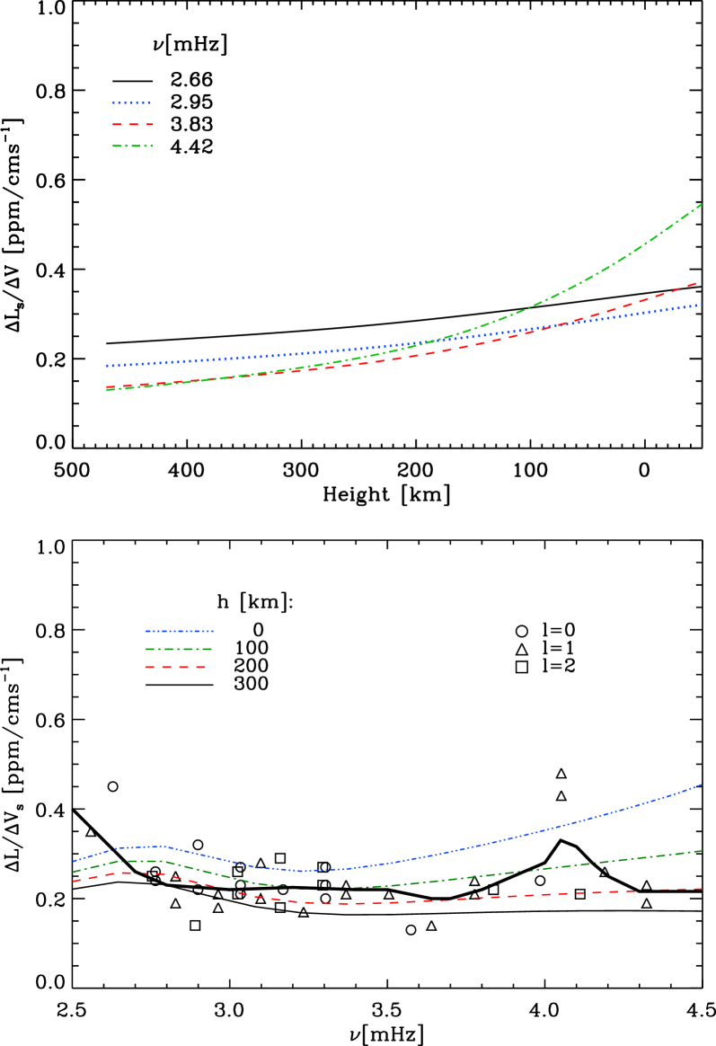
Figure 2: Top: Calculated amplitude ratios (see equation (15)) as a function of height in a solar model for modes with different frequency values. Bottom: Theoretical amplitude ratios (surface luminosity perturbation over velocity) for a solar model compared with observations by Schrijver et al. (1991). Computed results are depicted at different heights above the photosphere ($h$=0 km at $T=T_{\rm eff}$) The thick, solid curve indicates a running-mean average of the data (from Houdek et al. 1995).

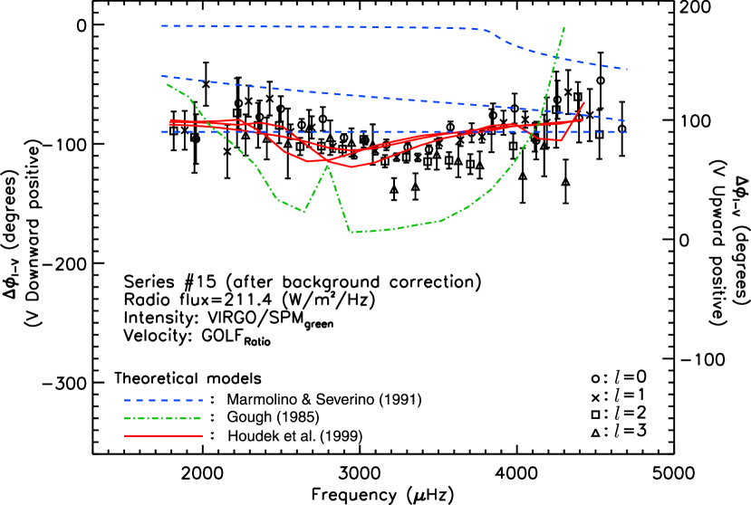
Figure 3: Intensity-velocity phase differences of low-degree p modes at the maximum of solar activity. Symbols are the results from intensity observations in the green channel of the VIRGO/SPM instrument on the SOHO spacecraft, and from contemporaneous velocity observations from the GOLF instrument. Theoretical results are depicted for three models: the dashed curves assume Newton’s cooling law for energy transfer with three different values for the damping times, the dot-dashed curve includes a local treatment of convection dynamics and the diffusion approximation to radiative transfer, and the solid curves are the results from the model discussed in Section 3 for three different sets of convection parameters (adopted from Jiménez 2002).

An additional useful property of the oscillations is the phase difference between intensity and velocity. Phase shifts between intensity observations from the VIRGO/SPM instrument and contemporaneous velocity measurements from the GOLF instrument (symbols with error bars) are plotted as function of frequency in Fig. 3 together with results from various model computations (curves). The dashed curves are the results from calculations by Marmolino & Severino (1991) who treated the energy transport with Newton’s cooling law assuming various values for the damping time; the dot-dashed curve is the result by Gough (1985) who used the diffusion approximation to radiative transfer and a local, time-dependent mixing-length model to estimate the turbulent fluxes. The solid curves are the results from the model discussed in Section 3 and for three different sets of convection parameters (Houdek et al. 1999). The latter results are in good agreement with the observations.
The results depicted in Figs 2 and 3 provide us with confidence that the pulsation computations reproduce the properties of the radial eigenfunctions in the outer atmospheric solar layers reasonably well.

5 Solar damping rates

Damping of stellar oscillations arises basically from two sources: processes influencing the momentum balance, and processes influencing the thermal energy equation. Each of these contributions can be divided further according to their physical origin, which was discussed in detail by Houdek et al. (1999).

Important processes that influence the thermal energy balance are nonadiabatic processes attributed to the modulation of the convective heat flux by the pulsation. This contribution is related to the way that convection modulates large-scale temperature perturbations induced by the pulsations which, together with the conventional $\kappa$-mechanism, influences pulsational stability.
Current models suggest that an important contribution that influences the momentum balance is the exchange of energy between the pulsation and the turbulent velocity field through dynamical effects of the fluctuating Reynolds stress. In fact, it is the modulation of the turbulent fluxes by the pulsations that seems to be the predominant mechanism responsible for the driving and damping of solar-type acoustic modes. It was first reported by Gough (1980) that the dynamical effects arising from the turbulent momentum flux perturbation $\delta p_{\rm t}$ contribute significantly to the damping $\Gamma$. Detailed analyses (Balmforth 1992a) reveal how damping is controlled largely by the phase difference between the momentum perturbation and the density perturbation. Therefore, turbulent pressure fluctuations must not be neglected in stability analyses of solar-type p modes.

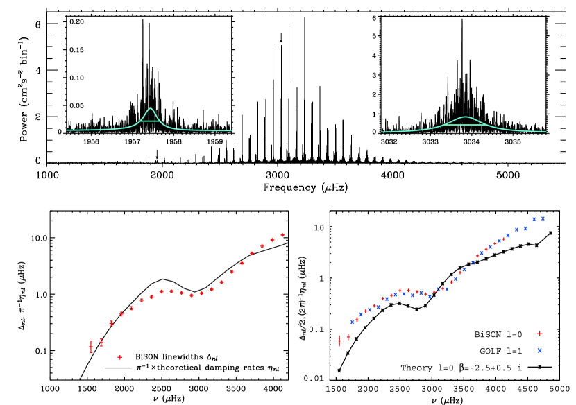
Figure 4: Top: Power spectrum of solar low-degree p modes obtained from a 3456-d data set collected by BiSON between 1991 and 2000 (Chaplin et al. 2005). The two insets show Lorentzian profile fits (and their full-width at half-maximum (FWHM); solid, blue curves) to the spectral peaks of radial modes with order $n=13$ (left) and $n=21$ (right); both spectral peaks are indicated by vertical arrows in the power spectrum. Bottom: The symbols in the left-hand panel are the measured BiSON linewidths $\Delta_{nl}=\Gamma_{nl}/2\pi$ (we denote the FWHM in unit of cyclic frequency by $\Delta_{nl}$) which are compared with the theoretical damping rates $\pi^{-1}\eta_{nl}$ (connected by the solid curve) obtained from the model computations of Section 3 (from Chaplin et al. 2005). In the right-hand panel theoretical results of $(2\pi)^{-1}\eta_{nl}$ (solid curve) by Dupret et al. (2004) are compared with observations of $\Delta_{nl}/2$ (symbols).

A comparison between the latest linewidth measurements (full-width at half-maximum) $\Delta_{nl}=\Gamma_{nl}/2\pi$ and theoretical damping rates is given in Fig. 4. The observational time series from BiSON (Chaplin et al. 2005) was obtained from a 3456-d data set and the linewidths of the temporal power spectrum (top panel) extend over many frequency bins $\hat{\delta}=1/2T_{\rm obs}$. In that case the linewidth in units of cyclic frequency is related to the damping rate according to

$$\Delta_{nl}=\pi^{-1}\eta_{nl}\,.$$ (16)

Recently Dupret et al. (2004, see also these proceedings) performed similar stability computations for the Sun using the time-dependent mixing-length formulation by Gabriel et al. (1975, 1998) which is based on the formulation by Unno (1967). The outcome of their computations is illustrated in the lower right panel of Fig. 4, which also shows the characteristic plateau near 2.8 mHz. It is, however, interesting to note that their findings suggest the fluctuating convective heat flux to be the main contribution to mode damping, whereas for the model results shown in the lower left panel of Fig. 4, which are based on Gough’s (1977a,b) convection formulation, it is predominantly the fluctuating Reynolds stress that makes all modes stable.

6 Excitation model and solar amplitudes

Because of the lack of a complete model for convection, the mixing-length formalism still represents the main method for computing the turbulent fluxes in the convectively unstable layers in a star. One of the assumptions in the mixing-length formulation is the Boussinesq approximation, which results in neglecting the acoustic wave generation by assuming the fluid to be incompressible. Consequently a separate model is needed to estimate the rate of the acoustic noise (energy supply rate) generated by the turbulence. The excitation process can be regarded as multipole acoustic radiation (Lighthill 1952). Acoustic radiation by turbulent multipole sources in the context of stellar aerodynamics has been considered by Unno & Kato (1962), Moore & Spiegel (1964), Unno (1964), Stein (1967), Goldreich & Keeley (1977), Bohn (1984), Osaki (1990), Goldreich & Kumar (1990), Balmforth (1992b), Goldreich, Murray & Kumar (1994), Musielak et al. (1994), Samadi & Goupil (2001) and Chaplin et al. (2005).

6.1 Excitation model

The mean amplitude $A$ of a mode is determined by a balance by the energy supply rated $P_{\rm f}$ from the turbulent velocity field and the thermal and mechanical dissipation rate characterized by the damping coefficient $\eta$. The procedure that we adopt to estimate $A$ is that of Chaplin et al. (2005), whose prescription follows that of Balmforth (1992b).

As in Section 2 we represent the linearized pulsation dynamics by the simplified equation

$$\rho\left(\frac{\partial^{2}\boldsymbol{\xi}}{\partial t^{2}}+2\eta\frac{\partial\boldsymbol{\xi}}{\partial t}+\mathcal{L}\boldsymbol{\xi}\right)=\boldsymbol{\mathcal{F}}(\boldsymbol{u})+\boldsymbol{\mathcal{G}}(s^{\prime})$$ (17)

for the displacement $\boldsymbol{\xi}(\boldsymbol{r},t)$, which is now also a function of radius $\boldsymbol{r}$, of a forced oscillation corresponding to a single radial mode satisfying the homogeneous equation

$${\cal L}\boldsymbol{\xi}(\boldsymbol{r})=\omega^{2}\boldsymbol{\xi}(\boldsymbol{r})$$ (18)

in which $\omega$ (and $\boldsymbol{\xi}$) are real and ${\cal L}$ is a linear spatial operator. The (inhomogeneous) fluctuating terms on the right-hand-side of equation (17) arise from the fluctuating Reynolds stresses

$$\boldsymbol{\cal F}(\boldsymbol{u})=\nabla\cdot(\rho\boldsymbol{u}\boldsymbol{u}-\langle\rho\boldsymbol{u}\boldsymbol{u}\rangle)$$ (19)

and from the fluctuating gas pressure (due to the fluctuating buoyancy force), represented by $\boldsymbol{\mathcal{G}}(s^{\prime})$, where $s^{\prime}$ is the Eulerian entropy fluctuation (Bohn 1984; Osaki 1990; Goldreich & Kumar 1990; Balmforth 1992b; Goldreich, Murray & Kumar 1994; Samadi & Goupil 2001). The latest numerical simulations by Stein et al. (2004) suggest that both forcing terms in equation (17) contribute to the energy supply rate $P_{\rm f}$ by about the same amount, a result that was also reported by Samadi et al. (2003) using the turbulent velocity field and anisotropy factors from numerical simulations (Stein & Nordlund 2001). In this paper we consider only the term of the fluctuating Reynolds stresses and because we use only radial modes, only the vertical component of $\boldsymbol{\cal F}$ is important,

$${\cal F}_{3}(u_{3})\simeq\frac{\partial}{\partial r}(\rho u^{2}_{3}-\langle\rho u^{2}_{3}\rangle)\,.$$ (20)

If we define the vertical component of the velocity correlation as $R_{33}=\langle u_{3}u_{3}\rangle$, its Fourier transform $\widehat{R}_{33}$ can be expressed in the Boussinesq-quasi-normal approximation (e.g. Batchelor 1953) as a function of the turbulent energy spectrum function $E(k,\omega)$:

$$\widehat{R}_{33}=\frac{\Psi E(k,\omega)}{12\pi k^{2}}\,,$$ (21)

where $k$ is a wavenumber and $\Psi$ is an anisotropy parameters given by

$$\Psi=\left[{2\Phi}/{3(\Phi-1)}\right]^{1/2}$$ (22)

which is unity for isotropic turbulence (Chaplin et al. 2005). This factor was neglected in previously published excitation models but it has to be included in a consistent computation of the acoustic energy supply rate. Following Stein (1967) we factorize the energy spectrum function into $E(k,\omega)=E(k)\Omega(\omega;\tau_{k})$, where $\tau_{k}=\lambda/ku_{k}$ is the correlation time-scale of eddies of size $\pi/k$ and velocity $u_{k}$; the correlation factor $\lambda$ is of order unity and accounts for uncertainties in defining $\tau_{k}$.

Figure 5: Comparison of the frequency factor $\tilde{\Omega}(\omega;\tau_{k})$ (see equation (24)) between hydrodynamical simulation results for solar convection (Stein & Nordlund 2001; symbols) and the Lorentzian frequency factor by Samadi et al. (2003) for two different values of the correlation factor $\lambda$ (solid and dashed curves). The results are plotted as function of frequency evaluated 0.99 Mm below the solar photosphere (adopted from Samadi et al. 2003).

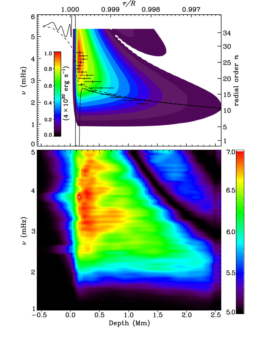
Figure 6: Top: The contours represent the integrand of the acoustic energy supply rate (23), multiplied by $I^{-1}{\rm d}r/{\rm d}\ln p$, and are plotted as function of frequency $\nu$ and the depth variable $z={\rm R}_{\odot}\!\!-\!r$. The plus symbols with (horizontal) error bars are the measured locations of the excitation regions by Chaplin & Appourchaux (1999). The solid and dashed curves denote the exact acoustic cutoff frequency and the approximation in an isothermal region, $c/2H_{p}$, where $c$ is the sound speed and $H_{p}$ is the pressure scale height. Bottom: Logarithm of integrand of the acoustic energy supply rate from Stein & Nordlund’s (2001) hydrodynamical simulations.

The energy supply rate is then given by (see Chaplin et al. 2005 for details)

$$P_{\rm f}=\frac{\pi}{9I}\int_{0}^{R}\ell^{3}\left(\Phi\Psi rp_{\rm t}\frac{\partial{\xi}_{r}}{\partial r}\right)^{2}{\cal S}(r;\omega)\,{\rm d}r\,,$$ (23)

with

$${\cal S}(r;\omega)=\int_{0}^{\infty}\kappa^{-2}\tilde{E}^{2}(\kappa)\tilde{\Omega}(\tau_{k};\omega)\,{\rm d}\kappa\,,$$ (24)

where $\kappa=k\ell/\pi$, $\ell$ is the mixing length, $R$ is surface radius, and $\xi_{r}$ is the normalized radial part of $\boldsymbol{\xi}$. The spectral function ${\cal S}$ accounts for contributions to $P_{\rm f}$ from the small-scale turbulence and includes the normalized spatial turbulent energy spectrum $\tilde{E}(k)$ and the frequency-dependent factor $\tilde{\Omega}(\tau_{k};\omega)$. For $\tilde{E}(k)$ it has been common to adopt either the Kolmogorov (Kolmogorov 1941) or the Spiegel spectrum (Spiegel 1962). The frequency-dependent factor $\tilde{\Omega}(\tau_{k};\omega)$ is still modelled in a very rudimentary way and we adopt two forms:
– the Gaussian factor (Stein 1967) ,

$$\tilde{\Omega}_{\rm G}(\omega;\tau_{k})=\frac{\tau_{k}}{\sqrt{2\pi}}\,{\rm e}^{-(\omega\tau_{k}/\sqrt{2})^{2}}\,;$$ (25)

– the Lorentzian factor (Gough 1977b; Samadi et al. 2003; Chaplin et al. 2005) ,

$$\tilde{\Omega}_{\rm L}(\omega;\tau_{k})=\frac{\tau_{k}}{\pi\sqrt{2\ln 2}}\,\frac{1}{1+(\omega\tau_{k}/\sqrt{2\ln 2})^{2}}\,.$$ (26)

The Lorentzian frequency factor is a result predicted for the largest, most-energetic eddies by the time-dependent mixing-length formulation of Gough (1977b). Recently, Samadi et al. (2003) reported that Stein & Nordlund’s hydrodynamical simulations also suggest a Lorentzian frequency factor (see Fig. 5), which decays more slowly with depth $z$ and frequency $\omega$ than the Gaussian factor. Consequently a substantial fraction to the integrand of equation (23) arises from eddies situated in the deeper layers of the Sun, resulting in a larger acoustic excitation rate $P_{\rm f}$.

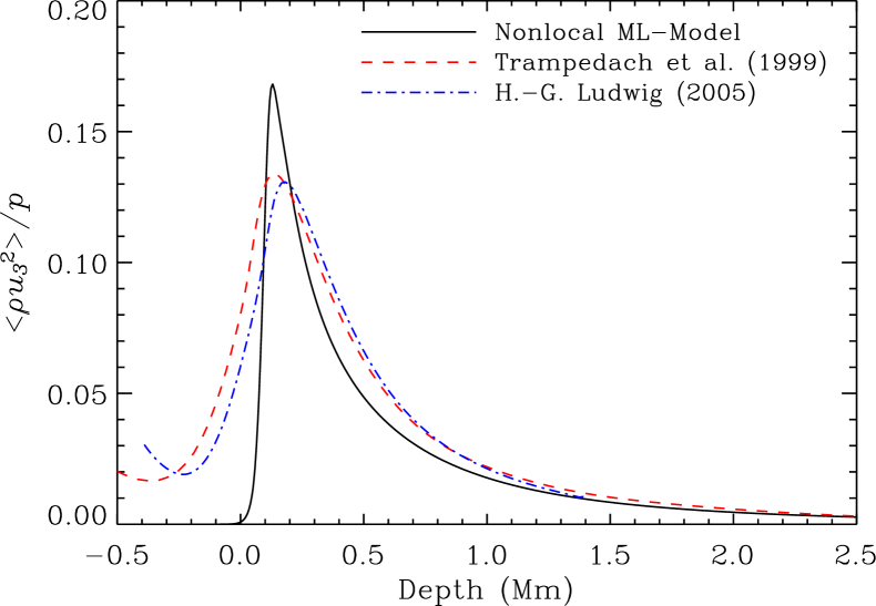
Figure 7: Reynolds stress as a function of the depth variable $z={\rm R}_{\odot}-r$ for various solar models. Results are shown for the nonlocal mixing-length model (solid, black curve) and from hydrodynamical simulations by Trampedach et al. (1999, dashed, red curve) and Ludwig (2005, dot-dashed, blue curve).

Another way to study the properties of the turbulent-excitation model is to compare the depth and frequency dependence of the integrand of $P_{\rm f}$ with solar measurements and with hydrodynamical simulations of the Sun. The results are depicted in Fig. 6: the contours in the top panel show the integrand of equation (23) multiplied by $I^{-1}$d$r$/d$\ln p$. The contours are compared with measurements of the locations of the driving regions by Chaplin & Appourchaux’s (1999), represented by the plus symbols with (horizontal) error bars. The modelled locations of the excitation regions are in good agreement with the observations, particularly for modes with frequencies larger than the acoustic cutoff frequency (these modes are therefore propagating). The cutoff frequency is the solid curve and the dashed curve is the isothermal approximation $c/2H_{p}$, where $c$ is the sound speed and $H_{p}$ is the pressure scale height. For these (propagating) modes the frequency dependence of $P_{\rm f}$ is predominantly determined by the turbulent spectrum (represented by the spectral function ${\cal S}$, cf. equation (24)). Modes with frequencies smaller than the acoustic cutoff frequency are evanescent, and their frequency dependence of $P_{\rm f}$ is predominantly determined by the shape of the eigenfunctions, i.e. by the term $(\partial\xi_{r}/\partial r)^{2}/I$, and consequently by the structure of the equilibrium model.

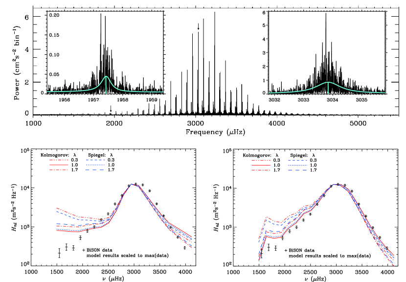
Figure 8: Top: Power spectrum of solar low-degree p modes obtained from a 3456-d data set by BiSON (Chaplin et al. 2005). The two insets show Lorentzian profile fits (and their heights $H$; solid, blue curves) to the spectral peaks of radial modes with order $n=13$ (left) and $n=21$ (right); both spectral peaks are indicated by vertical arrows in the power spectrum. Bottom: Radial mode peak heights, $H$, from observation and modelling. The crosses (with error bars) are well determined heights extracted from fits to the 3456-d BiSON spectrum. The curves show predicted heights $H$ for two turbulent spectra, due to Kolmogorov and Spiegel, with a Gaussian factor $\Omega_{\rm G}$, and assuming various values for the eddy correlation factor $\lambda$; they are scaled such that their maximum values agree with the maximum value of the data. Left-hand panel – the theoretical curves were computed using modelled values for both the forcing $P_{\rm f}$ and linear damping rates $\eta$. Right-hand panel – the theoretical curves were computed using the modelled values for the forcing $P_{\rm f}$ but with the damping rates replaced by $\pi\Delta$, where $\Delta$ are observed mode widths.

The lower panel of Fig. 6 shows the logarithm to the base 10 of the integrand of the excitation rate of the numerical simulations by Stein & Nordlund (2001). As for the model results (top panel), the extent of the driving regions decreases with frequency; however, the simulations show broader excitation regions than the model results. This is predominantly a result of the different spatial extents of the Reynolds stresses $\langle\rho u^{2}_{3}\rangle$ between the hydrodynamical simulations and the nonlocal mixing-length model. A plot of $\langle\rho u^{2}_{3}\rangle/p$ ($p$ is the total pressure) as a function of the depth variable $z={\rm R}_{\odot}-r$ is illustrated in Fig. 7. The Reynolds stress of the nonlocal mixing-length model shows a narrow peak near $z\simeq 120\,$km and falls off more rapidly with $z$ than the results from both hydrodynamical simulations. This leads to a smaller excitation rate for the mixing-length model compared with the hydrodynamical results and consequently the modelled heights $H$ need to be scaled with a scaling factor $\Lambda>1$ in order to reproduce the observed values of the mode peak heights (Chaplin et al. 2005).

Figure 9: Top: Predicted apparent velocity amplitudes (defined to be $\sqrt{2}$ times the rms value) for a model of $\alpha$ Cen A, computed according to equation (7). Bottom: Linear damping rates for a model of $\alpha$ Cen A, obtained by solving the fully nonadiabatic pulsation equations (14).

Figure 10: Top: Predicted apparent velocity amplitudes (defined to be $\sqrt{2}$ times the rms value) for a model of $\xi$ Hydrae, computed according to equation (7). Bottom: Linear damping rates for a model of $\xi$ Hydrae, obtained by solving the fully nonadiabatic pulsation equations (14) (adopted from Houdek & Gough 2002).

6.2 Solar amplitudes

Model predictions of the mode height $H$ were computed according to equation (8) assuming $\Phi$ to be constant; the value 1.13 was adopted because it produces the best fit to the linewidth data (cf. lower left panel of Fig. 4). The resulting values are joined by lines of various style in the lower panels of Fig. 8 for different values of the correlation factor $\lambda$ and for the two different forms of the spatial energy spectrum $\tilde{E}(k)$, in all cases with the Gaussian frequency factor given by equation (25). The BiSON measurements are rendered as crosses (with error bars). The maximum values of the theoretical results have been scaled to the maximum observed value. The values of the scaling factor $\Lambda$ by which we have multiplied the theoretical values are given in Chaplin et al. (2005). The scaled theoretical estimations of $H$ shown in the lower left-hand panel of the figure used modelled values of both the energy supply rate $P_{\rm f}$ and the linear damping rate $\eta$. They exceed the observed values at both low and high frequency, largely as a consequence of the modelled linewidths being larger than their measured counterparts at intermediate frequencies. This is demonstrated by comparison with the lower right-hand panel of Fig. 8, where predictions of $H$ have been made using the modelled energy supply rate but with the observed BiSON linewidths $\Delta$, rather than the modelled damping rates $\eta$. There is a dramatic improvement in the modelled spectral heights $H$, although agreement with observations remains imperfect. The discrepancy that remains when using observed linewidths is indicative of error in the equilibrium model and in the modelling of the energy supply rate $P_{\rm f}$. This comparison reveals that the principal error in the theory, at least for the Sun, rests in the calculation of the damping rates, particularly for low-order modes. These modes have upper turning points well below the region where most of the excitation takes place.
Chaplin et al. (2005) have also computed mode heights $H$ using the Lorentzian frequency factor (26), but have found that in that case the heights at low frequency are severely overestimated. This result comes about because the Lorentzian factor decreases too slowly with depth at constant frequency. This is particularly so for modes of lowest frequency, for which the Lorentzian is widest. Since it is not obvious where in the frequency spectrum the transition from a Lorentzian (largest most-energetic eddies) to a Gaussian (small-scale turbulence) frequency spectrum takes place, results are shown only for the purely Gaussian frequency factor.

7 Solar-like amplitudes in other stars

Fairly accurate measurements of solar-like oscillation amplitudes in other stars are available today from ground based observations (e.g. Kjeldsen et al. 2005; Bedding, these proceedings). Estimates of solar-like oscillation amplitudes in other stars were carried out by Christensen-Dalsgaard & Frandsen (1983), Kjeldsen & Bedding (1995), Houdek et al. (1999), Houdek & Gough (2002) and Samadi et al. (2005).

Table 2: Comparison of scaling laws and theoretical velocity estimates with the observations of solar-like oscillations. The quantity $\hat{V}_{\rm obs}$ is the typical observed maximum apparent velocity amplitude (defined to be $\sqrt{2}$ times the rms value), and $\hat{V}$ is the value obtained by the excitation theory, scaled to render $\hat{V}=\hat{\rm V}_{\odot}$ for the Sun. The solar value was taken to be $\hat{\rm V}_{\odot}$= 0.23 m s^-1 (from Houdek & Gough 2002).

Star	$M/{\rm M}_{\odot}$	$L/{\rm L}_{\odot}$	$T_{\rm e}/{\rm T}_{{\rm e}\odot}$	$L{\rm M}_{\odot}/{\rm L}_{\odot}M$	${\rm g}_{\odot}/g$	$\hat{V}/\hat{\rm V}_{\odot}$	$\hat{V}_{\rm obs}/\hat{\rm V}_{\odot}$
$\alpha$ Cen A	1.16	1.58	1.004	1.35	1.34	1.39	1.5a
$\beta$ Hyi	1.11	3.50	1.004	3.15	3.11	3.25	2.2b
Procyon	1.46	6.62	1.107	4.53	3.02	6.47	2.6c
$\xi\,$Hya	3.31	60.00	0.857	18.13	33.64	9.04	8.7d

                    ^afrom Bouchy & Carrier (2001), ^bfrom Bedding et al. (2001),                     ^cfrom Martic et al. (1999),     ^dFrandsen et al. (2002).

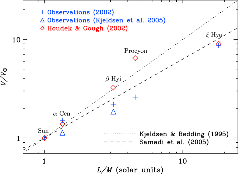
Figure 11: Predicted apparent velocity amplitudes (defined to be $\sqrt{2}$ times the rms value) as function of light-to-mass ratio for stochastically excited oscillations in other stars. Observations from several authors are plotted by the plus and triangle symbols. The theoretical estimates by Houdek & Gough (2002) are plotted as diamond symbols. The scaling law by Kjeldsen & Bedding (1995) is illustrated by the dotted line and results reported by Samadi et al. (2005) are indicated by the dashed line.

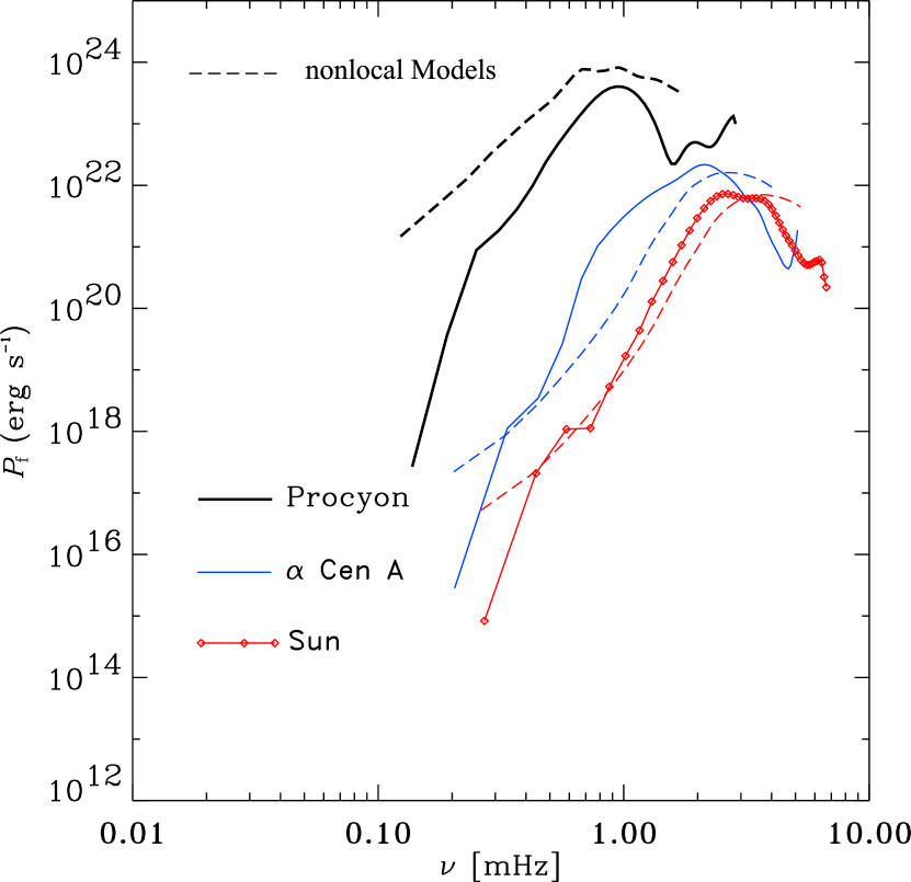
Figure 12: Acoustic excitation rates $P_{\rm f}$ of radial modes for the Sun and for the two solar-type stars $\alpha$ Cen A and Procyon. The solid curves are the results from numerical simulations by Stein et al. (2004) and the dashed curves are the model results of Sections 3 and 6. The model results have been scaled with a factor $\Lambda$ such as to obtain the same maximum solar value of $P_{\rm f}$ than that from the numerical simulations (adapted from Stein et al. 2004).

As in the solar case, damping rates for other stars are obtained from solving the eigenvalue problem (14) and from calculating the excitation rates from expression (23). With these estimates for $\eta$ and $P_{\rm f}$ Houdek & Gough (2002) predicted velocity amplitudes for several stars, using equation (7). Results for stochastically excited oscillation amplitudes and linear damping rates in the solar-like star $\alpha$ Cen A and in the sub-giant $\xi$ Hydrae are illustrated in Figs 9 and 10. Bedding et al. (2004) reported mode lifetimes for $\alpha$ Cen A between 1–2 days (see also Fletcher, these proceedings) which are in reasonable agreement with the theoretical estimates of about $1.7$ days for the most prominent modes (the mode lifetime $\tau\!=\!\eta^{-1}$; see lower panel of Fig. 9). For $\xi$ Hydrae, however, the theoretical mode lifetimes of the most prominent modes are $\tau\simeq 17$ days which are in stark contrast to the measured values of about 2–3 days by Stello et al. (2004, 2006), yet the estimated velocity amplitudes for $\xi\,$ Hydrae are in almost perfect agreement with the observations by Frandsen et al. (2002). The estimated velocity amplitudes, together with theoretical results for other solar-like oscillators, are compared with measurements from various observing campaigns and with the suggested scaling laws by Kjeldsen & Bedding (1995, 2001) in Table 2. For the cooler stars the theoretical results are in reasonable agreement with the observations. For the rather hotter star Procyon, however, the theoretical velocity amplitudes are severely overestimated (see Table 2).
This comparison between predicted and observed velocity amplitudes is illustrated in Fig. 11. The dotted line is the scaling law by Kjeldsen & Bedding (1995), and the dashed line is the scaling relation reported by Samadi et al. (2005) using the convective velocity profiles from numerical simulations (Stein & Nordlund 2001), a Lorentzian frequency factor in equation (24), and the theoretical damping rates from Houdek et al. (1999). For hotter stars they find better agreement with observations.

8 Comparison with numerical simulations

Recently Stein et al. (2004) reported stochastic excitation rates for radial p modes in various stars obtained from hydrodynamical simulations of their surface convection zones. By comparing the excitation rates between these simulation results and the model computations discussed in the previous sections, we can put some constraints on the modelled oscillation amplitudes. In Fig. 12 the excitation rates for the Sun and for the two solar-like pulsators $\alpha$ Cen A and Procyon are plotted versus frequency. The solid curves are the results from the numerical simulations and the dotted curves are the excitation rates obtained from equation (23). The theoretical values were multiplied with a scaling factor $\Lambda$ such as to obtain for the solar model the same maximum value of $P_{\rm f}$ than that from the numerical simulations. This allows us to compare the results for Procyon and $\alpha$ Cen A between the simulation ($P_{\rm sim}$) and model ($P_{\rm model}$) computations (from here on we omit the subscript f).

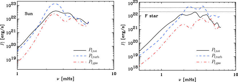
Figure 13: Total excitation rate $P_{\rm f,tot}$ and individual contributions from the turbulent $P_{\rm f,turb}$ and gas $P_{\rm f,gas}$ pressure fluctuations obtained from numerical simulations for a solar model (left panel) and for a model of an F star (right panel). For the solar model the two individual excitation sources are roughly similar in magnitude but for the hotter F star the driving from the Reynolds stress (turbulent pressure) fluctuations dominates. Partial cancellation between the Reynolds stress and gas pressure (buoyancy) fluctuations leads to a total excitation rate $P_{\rm f,tot}$ that is smaller (by a factor of about two in the F star, indicated by the two horizontal, dotted lines) than the contribution from the Reynolds stresses $P_{\rm f,turb}$ (adopted from Stein et al. 2004).

From this comparison (see Fig. 12) we obtain for Procyon

$$P_{\rm model}\simeq 2\times P_{\rm sim}\,,$$ (27)

and from Table 2 we obtain for the ratio between the modelled ($V_{\rm model}$) and observed ($V_{\rm obs}$) velocity amplitude for Procyon

$$V_{\rm model}\simeq 2.5\times V_{\rm obs}\,.$$ (28)

With the assumption that the numerical simulations provide the “correct” maximum value for the excitation rate $P=P_{\rm sim}$, we can estimate from the expressions $V=\sqrt{P/2\eta I}$ (see equation (7)), (27) and (28) the amount by which the modelled values of $P_{\rm model}$ and of $(2\eta I)^{-1}$ are at variance with the observations:

$$V_{\rm model}\simeq\sqrt{2}\times 1.77\times V_{\rm obs}\,,$$ (29)

suggesting that the modelled excitation rate $P_{\rm model}$ is too large by a factor of about two and the modelled value of $\sqrt{2\eta I}$ too small by a factor of about 1.77. In Section 4 we concluded that the modelled eigenfunctions, and therefore mode inertia $I$, reproduce the observations reasonably well. Consequently we can argue that it is predominantly the theoretical damping rate $\eta$ in $\sqrt{2\eta I}$ which contributes to the factor of 1.77, i.e. $\eta$ is too small (or the modelled mode lifetime too large).
A similar analysis can be done with $\alpha$ Cen A, for which we obtain from Fig.12 and Table 2:

$$V_{\rm model}\simeq\sqrt{0.8}\times 1.04\times V_{\rm obs}\,,$$ (30)

suggesting that for this star the modelled damping rates $\eta$ are in good agreement with the observations (see also lower panel of Fig.9).

It is interesting to note that the numerical simulations by Stein et al. (2004) show partial cancellation between the two excitation sources ${\boldsymbol{\cal F}}(\boldsymbol{u})$ and ${\boldsymbol{\cal G}}(s^{\prime})$ (see equation (17)) arising from the fluctuating turbulent pressure (Reynolds stresses) and gas pressure (buoyancy force); cancellation between acoustic multipole sources was discussed before by Goldreich & Kumar (1990) and Osaki (1990). This effect is illustrated in Fig. 13 which shows the total excitation rate $P_{\rm f,tot}$ and the individual contributions $P_{\rm f,turb}$ and $P_{\rm f,gas}$ from the turbulent and gas pressure fluctuations obtained from numerical simulations of the surface convection in the Sun and in a hotter star of spectral type F, the latter having model properties that are similar to that of Procyon. It is particularly striking that for the F star the effect of this partial cancellation leads, for the most prominent modes, to a total excitation rate $P_{\rm f,tot}$ which is, on average, by a factor of about two smaller than the excitation rate from only the turbulent pressure fluctuations $P_{\rm f,turb}$ (illustrated by the two dotted horizontal lines). One is therefore tempted to argue that the overestimated values of the modelled excitation rate $P_{\rm f}$ in Procyon (which is an F5 star) could be partially attributed to having neglected the gas pressure fluctuations in equation (17) and more importantly its cancellation effect with the turbulent pressure fluctuations. Including a formulation of this cancellation effect into the excitation model of Section 6.1 could bring the estimated velocity amplitudes, particularly for hotter stars, in better agreement with the observations.

References

- (1) Balmforth N.J. 1992a, MNRAS 255, 603
- (2) Balmforth N.J. 1992b, MNRAS 255, 639
- (3) Batchelor G.K., 1953, Homogeneous Turbulence, Cambridge University Press, Cambridge
- (4) Bedding T.R., Butler R.P., Kjeldsen H., et al. 2001, ApJ 549, L105
- (5) Bedding T.R., Kjeldsen H., Butler R.P., et al. 2004, ApJ 614, 380
- (6) Bohn H.U., 1984, A&A 136, 338
- (7) Bouchy F., Carrier F. 2001, A&A 374, L5
- (8) Chaplin W.J., Appourchaux T. 1999, MNRAS 309, 761
- (9) Chaplin W.J., Houdek G., Elsworth Y., Gough D.O., Isaak, G.R., New R. 2005, MNRAS 360, 859
- (10) Chaplin W.J., Elsworth Y., Isaak G.R., Lines R., McLeod C.P., Miller B.A., New R. 1998, MNRAS 298, L7
- (11) Christensen-Dalsgaard J., Gough D. 1982, MNRAS 198, 141
- (12) Christensen-Dalsgaard J., Frandsen S. 1983, Solar Phys. 82, 469
- (13) Dupret M.-A., Grigahcène A., Garrido R., Gabriel M., Noels A., in Proc. SOHO 14/GONG 2004 Workshop, ed. D.Danesy, ESA SP-559, (Noordwijk: ESTEC), 207
- (14) Frandsen S., Carrier F., Aerts C., et al. 2002, A&A 394, L5
- (15) Gabriel M., Scuflaire R., Noels A, Boury A. 1975, A&A 208, 122
- (16) Gabriel M., in Proc. SOHO 6/GONG 98 Workshop, eds S. Korzennik, A. Wilson, ESA SP-418 (Noordwijk: ESTEC), 863
- (17) Goldreich P., Keeley D.A. 1977, ApJ 212, 243
- (18) Goldreich P., Kumar P. 1990, ApJ 363, 694
- (19) Goldreich P., Murray N., Kumar P. 1994, ApJ 423, 466
- (20) Gough D.O. 1977a, in Problems of stellar convection, eds E. Spiegel, J.-P. Zahn (Berlin: Springer-Verlag), 15
- (21) Gough D.O. 1977b, ApJ 214, 196
- (22) Gough D.O. 1980, in Nonradial and Nonlinear Stellar Pulsation, eds H.A. Hill, W.A. Dziembowski, (Berlin: Springer-Verlag), 273
- (23) Gough D.O. 1985, in Proc. Future Missions in Solar, Heliospheric and Space Plasma Physics, eds E. Rolfe, B. Battirck, ESA SP-235, (Noordwijk:ESTEC), 183
- (24) Houdek G., Balmforth N., Christensen-Dalsgaard J. 1995, in Proc. 4th SOHO Workshop, eds J.T. Hoeksema, V. Domingo, B. Fleck, B. Battrick, ESA SP-376, Vol. 2, (Noordwijk: ESTEC), 447
- (25) Houdek G., Balmforth N.J., Christensen-Dalsgaard J., Gough D.O. 1999, A&A 351, 582
- (26) Houdek G., Gough D.O. 2002, MNRAS 336, L65
- (27) Jiménez A., ApJ 581, 736
- (28) Kjeldsen H., Bedding T.R. 1995, A&A 293, 87
- (29) Kjeldsen H., Bedding T.R., 2001, in Proc. SOHO 10/GONG 2000 Workshop, ed. A. Wilson, ESA SP-464, (Noordwijk: ESTEC), 361
- (30) Kjeldsen H., Bedding T.R., Butler R.P., et al. 2005, ApJ 635, 1281
- (31) Kolmogorov A.N. 1941, Dokl. Akad. Nauk SSSR, 30, 299
- (32) Kosovichev A.G. 1995, in Proc. of Fourth SOHO Workshop, eds J.T. Hoeksama, V. Domingo, B. Fleck, ESA SP-376, vol.2, (Noordwijk: ESTEC), 165
- (33) Libbrecht K.G. 1988, ApJ 334, 510
- (34) Lighthill M.J. 1952, Proc. Roy. Soc. London A211, 564
- (35) Ludwig H.-G. 2005, personal communication
- (36) Marmolino C., Stebbins R.T. 1989, Solar Phys. 124, 23
- (37) Musielak Z.E., Rosner R., Stein R.F., Ulmschneider P. 1994, ApJ 423, 474
- (38) Martic M., Schmitt J., Lebrun J.-C., Barban C., Connes P., Bouchy F., Michel E., Baglin A., Appourchaux T., Bertaux J.-L. 1999, A&A 351, 993
- (39) Moore D.W., Spiegel E.A. 1964, ApJ 139, 48
- (40) Osaki Y. 1990, in Progress of Seismology of the Sun and Stars, eds Y. Osaki Y., H. Shibahashi, (Berlin: Springer-Verlag), 145
- (41) Samadi R., Goupil M.-J. 2001, A&A 370, 136
- (42) Samadi R., Nordlund Å., Stein R.F., Goupil M.-J., Roxburgh I., 2003, A&A 404, 1129
- (43) Samadi R., Goupil M.-J., Alecian E., et al. 2005, J. Astrophys Astr. 26, 171
- (44) Schrijver C.J., Jiménez A., Däppen W. 1991, A&A 251, 655
- (45) Spiegel E. 1962, J. Geophys. Res. 67, 3063
- (46) Stein R.F. 1967, Solar Phys. 2, 385
- (47) Stein R.F., Nordlund Å. 2001, ApJ 546, 585
- (48) Stein R., Georgobani D., Trampedach R., Ludwig H.-G., Nordlund Å. 2004, Solar Phys. 220, 229
- (49) Stello D., Kjeldsen H., Bedding T.R., et al. 2004, Solar Phys. 200, 207
- (50) Stello D., Kjeldsen H., Bedding T.R., Buzasi D. 2006, A&A 448, 709
- (51) Toutain T., Appourchaux T., Baudin F., et al. 1997, Solar Phys. 172, 311
- (52) Trampedach R., Stein R.F., Christensen-Dalsgaard J., Nordlund Å. 1999, in Theory and Tests of Convection in Stellar Structure, eds A. Giménez, E.F. Guinan, B. Montesinos, ASP Conf. Ser. 173, 233
- (53) Unno W. 1964, Trans. Int. astr. Un. XII(B), 555
- (54) Unno W. 1967, PASJ 19, 140
- (55) Unno W., Kato S. 1962, PASJ 14, 416
- (56) Unno W., Spiegel E.A. 1966, PASJ 18, 85