The formation and gas content of high redshift galaxies and minihalos

Abstract

We investigate the suppression of the baryon density fluctuations compared to the dark matter in the linear regime. Previous calculations predict that the suppression occurs up to a characteristic mass scale of $\sim 10^{6}$ M_⊙, which suggests that pressure has a central role in determining the properties of the first luminous objects at early times. We show that the expected characteristic mass scale is in fact substantially lower (by a factor of $\sim 3$–10, depending on redshift), and thus the effect of baryonic pressure on the formation of galaxies up to reionization is only moderate. This result is due to the influence on perturbation growth of the high pressure that prevailed in the period from cosmic recombination to $z\sim 200$, when the gas began to cool adiabatically and the pressure then dropped. At $z\sim 10$ the suppression of the baryon fluctuations is still sensitive to the history of pressure in this high-redshift era. We calculate the fraction of the cosmic gas that is in minihalos and find that it is substantially higher than would be expected with the previously-estimated characteristic mass. Expanding our investigation to the non-linear regime, we calculate in detail the spherical collapse of high-redshift objects in a $\Lambda$CDM universe. We include the gravitational contributions of the baryons and radiation and the memory of their kinematic coupling before recombination. We use our results to predict a more accurate halo mass function as a function of redshift.

1 Introduction

The detection of the cosmic microwave background (CMB) temperature anisotropies (Bennett et al., 1996) confirmed the notion that the present-day galaxies and large-scale structure (LSS) evolved from the primordial inhomogeneities in the density distribution at very early times. After cosmic recombination, the gas decoupled from its mechanical drag on the CMB, and the baryons subsequently began to fall into the pre-existing gravitational potential wells of the dark matter. Regions that were denser than average collapsed and formed bound halos. First the smallest, least massive objects collapsed, and later, larger objects formed through a mixture of mergers and accretion. The formation and properties particularly of early galaxies at high redshift are being actively studied in anticipation of many expected observational probes (e.g., Barkana & Loeb, 2001; Barkana, 2006).

A well-known solution for the collapse of a halo that consists of dark matter only in an Einstein de Sitter (EdS) universe was presented by Gunn & Gott (1972). This solution considers a spherical region initially with a small uniform overdensity compared to the background universe. As the universe expands, the overdensity expands slower than the background until it reaches a maximum radius, turns around, and collapses. The critical overdensity, in the corresponding linearly-extrapolated calculation, marks the collapse time of a dark matter halo in this case as $\delta_{c}=1.686$, a value that does not depend on the halo mass or collapse redshift. The mathematical solution gives a singularity as the final state, but physically we know that even a small initial asymmetry will make the object stabilize with a finite size after reaching a virial equilibrium between motion and gravity.

Extensive work has been done on spherical collapse models, especially models that include a cosmological constant or a dark energy background (e.g., Lahav et al., 1991; Deshingkar et al., 2001; Lokas & Hoffman, 2001; Horellou & Berge, 2005; Maor & Lahav, 2005; Wang, 2005); in particular, the cosmological constant $\Lambda$ changes the above value of overdensity ($\delta_{c}$) by about $0.6\%$. In addition, many numerical simulations of the formation of primordial objects at $z\sim 20$–30 have been performed. However, the earliest stars formed at $z\sim 65$ (Naoz, Noter & Barkana, 2006), and even for a halo that collapsed at $z\sim 30$, $\delta$ must have started significantly non-linear ($\sim 9\%$) even for a simulation that begins as early as $z\sim 600$.

With the $\Lambda$CDM cosmological parameters (Spergel et al., 2006), the contribution of the photons to the expansion of the universe cannot be neglected when considering the formation of the first objects (Naoz, Noter & Barkana, 2006). Moreover, the baryons have a non-negligible contribution compared to the dark matter, and their different evolution must be included in the collapse process.

When considering the formation and properties of the first luminous objects, we must investigate the relation between the baryon and the dark matter fluctuations. Gnedin & Hui (1998) defined a fiducial “filtering mass” that describes the highest mass at which the baryonic pressure still manages to suppress the linear baryonic fluctuations significantly. Gnedin (2000) extended the usefulness of the filtering mass to the fully non-linear regime by showing that it is also related to another characteristic mass scale – the largest halo mass for which the gas content is substantially suppressed compared to the cosmic fraction. As we show below, if we follow previous calculations (Gnedin & Hui, 1998; Gnedin, 2000; Gnedin et al., 2003), we find a characteristic mass at high redshift of $\sim 10^{6}M_{\odot}$, approximately constant at $z\ga 60$ and decreasing only slowly with time afterwards. This is somewhat larger than the mass scale of the first objects and suggests a potent effect on the formation of the first objects.

Here we present an improved calculation of the characteristic mass that is mainly based on the improved calculation of the baryon density and temperature fluctuations that we presented in Naoz & Barkana (2005). We first review the basic equations of linear perturbation growth (Section 2.1). We then divide the power spectrum into several different ranges of scales that are associated with large-scale structure (Section 2.2), the filtering scale (Section 2.3), and small scales (Section 2.4). Note that we define the filtering mass with a different normalization than in previous works, as explained in Section 2.3. For completeness we compare our calculation to the older, inaccurate approximation of a spatially-uniform sound speed along with other approximations (Sections 2.5 and 2.6). We use our results for the filtering mass to estimate the gas fraction in minihalos (Section 2.7). In Section 3 we calculate in detail the critical overdensity for collapse of halos that form at very high redshifts, following the evolution of perturbations outside the horizon (Section 3.1) and inside it (Section 3.2). We also predict the halo abundance at different redshifts (Section 3.3). Finally, we summarize and discuss our results in Section 4.

Our calculations are made in a $\Lambda$CDM universe, including dark matter, baryons, radiation, and a cosmological constant. We assume cosmological parameters matching the three year WMAP data together with weak lensing observations (Spergel et al., 2006), i.e., $\Omega_{m}=0.299$, $\Omega_{\Lambda}=0.74$, $\Omega_{b}=0.0478$, $h=0.687$, $n=0.953$ and $\sigma_{8}=0.826$. We also consider the effect of current uncertainties in the values of cosmological parameters on some of our results, by comparing to the results with a different cosmological parameter set specified by Viel et al. (2006): $\Omega_{m}=0.253$, $\Omega_{\Lambda}=0.747$, $\Omega_{b}=0.0425$, $h=0.723$, $n=0.957$ and $\sigma_{8}=0.785$. These parameters represent typical 1-$\sigma$ errors, in terms of the parameter uncertainties given by Spergel et al. (2006).

2 Linear Growth of Perturbations

2.1 The Basic Equations

Naoz & Barkana (2005) showed that the baryonic sound speed varies spatially, so that the baryon temperature and density fluctuations must be tracked separately. Thus, the evolution of the linear density fluctuations of the dark matter ($\delta_{\mathrm{dm}}$) and the baryons ($\delta_{\mathrm{b}}$) is described by two coupled second-order differential equations:

$$\ddot{\delta}_{\mathrm{dm}}+2H\dot{\delta}_{\mathrm{dm}} = \frac{3}{2}H_{0}^{2}\frac{\Omega_{m}}{a^{3}}\left(f_{\mathrm{b}}\delta_{\mathrm{b}}+f_{\mathrm{dm}}\delta_{\mathrm{dm}}\right)\ ,$$ (1)

$$\ddot{\delta}_{\mathrm{b}}+2H\dot{\delta}_{\mathrm{b}} = \frac{3}{2}H_{0}^{2}\frac{\Omega_{m}}{a^{3}}\left(f_{\mathrm{b}}\delta_{\mathrm{b}}+f_{\mathrm{dm}}\delta_{\mathrm{dm}}\right)-\frac{k^{2}}{a^{2}}\frac{k_{B}\bar{T}}{\mu}\left(\delta_{\mathrm{b}}+\delta_{T}\right)\ ,$$

where $\Omega_{m}$ is the present matter density as a fraction of the critical density, $k$ is the comoving wavenumber, $a$ is the scale factor, $\mu$ is the mean molecular weight, $H_{0}$ marks the present value of the Hubble constant $H$, and $\bar{T}$ and $\delta_{T}$ are the mean baryon temperature and its dimensionless fluctuation, respectively. These equations can be derived by linearizing the continuity, Euler, and Poisson equations. The baryon equation includes a pressure term whose form comes from the equation of state of an ideal gas. The linear evolution of the temperature fluctuations is given by (Barkana & Loeb, 2005; Naoz & Barkana, 2005)

$$\frac{d\delta_{T}}{dt}=\frac{2}{3}\frac{d\delta_{\mathrm{b}}}{dt}+\frac{x_{e}(t)}{t_{\gamma}}a^{-4}\left\{\delta_{\gamma}\left(\frac{\bar{T}_{\gamma}}{\bar{T}}-1\right)+\frac{\bar{T}_{\gamma}}{\bar{T}}\left(\delta_{T_{\gamma}}-\delta_{T}\right)\right\}\ ,$$ (2)

where $x_{e}(t)$ is the electron fraction out of the total number density of gas particles at time $t$, $\delta_{\gamma}$ is the photon density fluctuation, $t_{\gamma}=8.55\times 10^{-13}{\mathrm{yr}}^{-1}$, and $T_{\gamma}$ and $\delta_{T_{\gamma}}$ are the mean photon temperature and its dimensionless fluctuation, respectively. Equation (2) results from the first law of thermodynamics, where in the post-recombination era before the formation of galaxies, the only external heating arises from Compton scattering of the remaining free electrons with CMB photons. The first term of equation (2) comes from the adiabatic cooling or heating of the gas, while the second term is the result of the Compton interaction. Note that prior analyses (e.g., Peebles, 1980; Ma & Bertschinger, 1995) had assumed a spatially uniform speed of sound for the gas, but this assumption is inaccurate.

It is often useful to express the evolution in terms of two linear combinations of the dark matter and baryon fluctuations. Defining $\delta_{\mathrm{tot}}=f_{\mathrm{b}}\delta_{\mathrm{b}}+f_{\mathrm{dm}}\delta_{\mathrm{dm}}$ (in terms of the cosmic baryon and dark matter mass fractions $f_{\mathrm{b}}$ and $f_{\mathrm{dm}}$) and $\Delta=\delta_{\mathrm{b}}-\delta_{\mathrm{tot}}$ (following the derivation in Barkana & Loeb, 2005), and using equations (1) we can write two differential equations that describe the evolution of $\delta_{\mathrm{tot}}$ and $\Delta$:

$$\ddot{\delta}_{\mathrm{tot}}+2H\dot{\delta}_{\mathrm{tot}} = \frac{3}{2}H_{0}^{2}\frac{\Omega_{m}}{a^{3}}\delta_{\mathrm{tot}}-f_{\mathrm{b}}\frac{k^{2}}{a^{2}}\frac{k_{B}\bar{T}}{\mu}\left(\delta_{\mathrm{tot}}+\Delta+\delta_{T}\right)\ ,$$

$$\ddot{\Delta}+2H\dot{\Delta} = -f_{\mathrm{dm}}\frac{k^{2}}{a^{2}}\frac{k_{B}\bar{T}}{\mu}\left(\delta_{\mathrm{tot}}+\Delta+\delta_{T}\right)\ .$$ (3)

Note that the gravitational force depends directly on $\delta_{\mathrm{tot}}$, which is the fluctuation in the total matter density, while $\Delta$ describes the difference between the baryon fluctuations and $\delta_{\mathrm{tot}}$. Before recombination, the baryons are dynamically strongly coupled to the photons while the dark matter fluctuations continue to grow independently. At lower redshifts the dominant contribution to the baryon fluctuation growth is the gravitational attraction to the dark matter gravitational wells (e.g., see Figure 1 in Naoz & Barkana (2005)).

2.2 Large-Scale Structure: Small-$k$ Limit

In the small-$k$ limit, the pressure terms can be neglected and equations (2.1) can be approximated as (following the derivation in Barkana & Loeb, 2005)

$$\ddot{\delta}_{\mathrm{tot}}+2H\dot{\delta}_{\mathrm{tot}} = \frac{3}{2}H_{0}^{2}\frac{\Omega_{m}}{a^{3}}\delta_{\mathrm{tot}}\ ,$$ (4)

$$\ddot{\Delta}+2H\dot{\Delta} = 0\ .$$

Each of these equations has two independent solutions. Assuming that the universe is accurately described as EdS before reionization, these solutions are simple. The solutions for the $\delta_{\mathrm{tot}}$ equation are growing and decaying modes $D_{\mathrm{tot},1}\propto a$ and $D_{\mathrm{tot},2}\propto a^{-3/2}$, while for the $\Delta$ equation we obtain $D_{\Delta,1}\propto 1$ and $D_{\Delta,2}\propto a^{-1/2}$. Moreover, with standard inflationary initial conditions, equations (4) satisfy $\Delta(k)\propto\delta_{\mathrm{tot}}(k)$ at a given redshift. In other words, the relation between $\Delta$ and $\delta_{\mathrm{tot}}$ is independent of wavenumber, for the range of redshifts and $k$ values that we are considering here. We therefore find it useful to define

$$r_{\rm LSS}\equiv\frac{\Delta}{\delta_{\mathrm{tot}}}\ ,$$ (5)

in terms of the solutions of equations (4) in the large-scale structure regime. The ratio $r_{\rm LSS}$ (which is negative) is independent of $k$ in this regime, and its magnitude decreases in time approximately $\propto 1/a$, since $\Delta$ is roughly constant and $\delta_{\mathrm{tot}}$ is dominated by the growing mode $\propto a$. Figure 1 (top panel) shows $|r_{\rm LSS}|$ as a function of redshift in the regime of large-scale structure. Although $|r_{\rm LSS}|$ decreases as $z\to 0$, the initial difference between the dark matter and the baryon fluctuations has a large effect on the filtering mass even at $z<10$, as we show below. The small-$k$ regime ($k\ll k_{F}$) can be seen in Figure 1 (bottom panel), in terms of the filtering wavenumber $k_{F}$ which is defined precisely in the following subsection. Note that remnants of the acoustic oscillations in the photon-baryon plasma can be seen on the largest scales ($k/k_{F}\sim 10^{-4}$, which corresponds to comoving $k\sim 0.01$–0.1 Mpc^-1), but these are much larger scales than those of high-redshift halos and the oscillations do not affect our results.

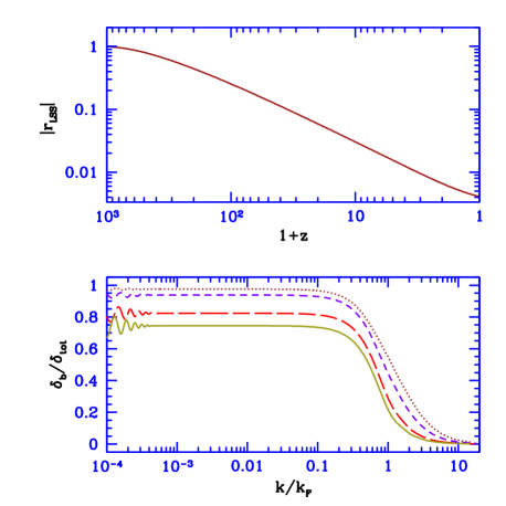
Figure 1: The top panel shows $|r_{\rm LSS}|$ (equation (5)) versus redshift. The bottom panel shows the baryon to total fluctuation ratio versus $k/k_{F}$ for various redshifts. We consider, from bottom to top, $z=100$, 65, 20, and 7.

A good numerical fit for $r_{\rm LSS}$ in the redshift range of $z=7-150$ is given by

$$r_{\rm LSS}=\frac{\alpha_{1}(\Omega_{m})}{a}+\frac{\alpha_{2}(\Omega_{m})}{a^{3/2}}+\alpha_{3}(\Omega_{m})\ ,$$ (6)

where the form is motivated by the definition of $r_{\rm LSS}$ (equation (5)) and the EdS solutions of equations (4). The fitted coefficients are

$$\alpha_{1}(\Omega_{m}) = 10^{-4}\times(-1.99\,\Omega_{m}^{2}+2.41\,\Omega_{m}+0.21)\ ,$$ (7)

$$\alpha_{2}(\Omega_{m}) = 10^{-3}\times(6.37\,\Omega_{m}^{2}-6.99\,\Omega_{m}-1.76)\ ,$$

$$\alpha_{3}(\Omega_{m}) = 10^{-2}\times(-1.83\,\Omega_{m}^{2}+2.4\,\Omega_{m}-0.54)\ ,$$

where the maximum residual error of the fit is $0.2\%$, over the range $\Omega_{m}=$0.25–0.4 in $\Lambda$CDM.

2.3 The Filtering Scale

In a $\Lambda$CDM universe, virialized CDM halos form on extremely small scales at extremely early times. The minimum mass scale on which galaxies form within these halos is determined through a combination of two physical properties of the infalling gas. These are cooling and pressure, and each produces a characteristic minimum scale, so that the larger of the two scales becomes the dominant factor that determines the minimum mass of star-forming halos.

During the gravitational collapse, the gas potential energy is transformed into kinetic and thermal energy through virialization and adiabatic compression. Unless the gas is able to dissipate its thermal energy with an effective cooling mechanism, the temperature will continue to rise, allowing the increasing pressure to halt the collapse. At very high redshifts, before metals were produced in supernovae and efficiently distributed in the intergalactic medium, the only cooling mechanism at temperatures below 10,000 K was cooling by molecular hydrogen, which itself is efficient only above a few hundred K. Thus, the first objects are expected to be fairly massive. Numerical calculations and simulations have shown that the minimum cooling mass is $\sim 10^{5}M_{\odot}$ at $z\sim 100$ and increases with time (Tegmark, 1997; Abel et al., 2002; Fuller, 2000; Yoshida, 2005). An object more massive than this minimum mass, after it goes through the virialization process, will cool and collapse further, producing high-density clumps in which stars can form.

Haiman et al. (1997) showed that the UV flux needed to dissociate H₂ in a collapsing environment is lower by more than two orders of magnitude than the flux that is necessary to reionize the universe. Therefore, once stars reach a certain abundance, the formation of stars through H₂ cooling is suppressed, and atomic cooling becomes the only available mechanism. This mechanism requires a much higher virial temperature ($T_{vir}\geq 10^{4}K$) which is associated with a halo mass of $\sim 10^{8}M_{\odot}$. Therefore, in order to study the first generations of objects we must consider halo masses of $\sim 10^{5}-10^{8}M_{\odot}$ (see also the review by Barkana (2006)).

On large scales (small wavenumbers) gravity dominates halo formation and pressure can be neglected. On small scales, on the other hand, the pressure dominates, and the baryon density fluctuations are suppressed compared to the dark matter fluctuations. The relative force balance at a given time can be characterized by the Jeans scale, which is the minimum scale on which a small perturbation will grow due to gravity overcoming the pressure gradient. If the gas has a uniform sound speed $c_{s}$, then the comoving Jeans wavenumber is

$$k_{J}=\frac{a}{c_{s}}\sqrt{4\pi G\bar{\rho}}\ .$$ (8)

Once the universe is matter-dominated, the Jeans scale is constant in time as long as $T\sim 1/a$, i.e., as long as the Compton scattering of the CMB with the residual free electrons after cosmic recombination keeps the gas temperature coupled to that of the CMB. At redshift $z\sim 200$ the gas temperature decouples from the CMB temperature and the Jeans scale decreases with time as the gas cools adiabatically. Any halo more massive than the Jeans mass can begin to collapse despite the pressure gradients. Figure 3 is a reminder that the Jeans mass (dotted curve) is in the range $10^{4}$– $10^{5}M_{\odot}$ during the formation of the earliest generations of galaxies.

The Jeans mass is related only to the evolution of perturbations at a given time. When the Jeans mass itself varies with time, the overall suppression of the growth of perturbations depends on a time-averaged Jeans mass. Following Gnedin & Hui (1998), we define a “filtering” scale and use it to identify the largest scale on which the baryon fluctuations are substantially suppressed compared to those of the dark matter. While Gnedin & Hui (1998) assumed a spatially-uniform sound speed and made a number of other approximations (see Section 2.5), we calculate here the fitering scale obtained from the exact numerical solution of equations (1). In particular, our initial conditions at high redshift account for the coupling of the baryons and photons, i.e., $\delta_{\mathrm{b}}\ll\delta_{\mathrm{dm}}$ up to cosmic recombination.

We define the filtering wavenumber $k_{F}$ based on the scale at which the baryon-to-total fluctuation ratio drops substantially below its value on large scales. Thus, we expand this ratio up to linear order in $k^{2}$, and write the expansion in the following form:

$$\frac{\delta_{\mathrm{b}}}{\delta_{\mathrm{tot}}}=1-\frac{k^{2}}{k_{F}^{2}}+r_{\rm LSS}\ ,$$ (9)

where $r_{\rm LSS}$ was defined in equation (5). Our definition of $k_{F}$ is a generalization of that by Gnedin & Hui (1998), who did not include the $r_{\rm LSS}$ term. To find $k_{F}$ in our more general case we first write it in the form:

$$k^{2}_{F}(t)=\frac{\delta_{\mathrm{tot}}(t)}{u(t)}\ ,$$ (10)

where $u(t)$ is to be determined. Substituting the expansion into equations (1) and (4), we obtain an equation for $u$:

$$\ddot{u}+2H\dot{u}=f_{\mathrm{dm}}\frac{1}{a^{2}}\frac{k_{B}\bar{T}}{\mu}\left(\delta_{\mathrm{tot}}+r_{\rm LSS}\delta_{\mathrm{tot}}+\delta_{T}\right)\ ,$$ (11)

where we have neglected terms of higher order in $k^{2}$. We can solve this equation to find the parameter $u$:

$$u(t)=\int^{t}_{t_{\rm rec}}\frac{dt^{\prime\prime}}{a^{2}(t^{\prime\prime})}\int_{t_{\rm rec}}^{t^{\prime\prime}}dt^{\prime}f_{\mathrm{dm}}\frac{k_{B}\bar{T}(t^{\prime})}{\mu}$$

$$\ \ \ \times\left(\delta_{\mathrm{tot}}(t^{\prime})+r_{\rm LSS}(t^{\prime})\delta_{\mathrm{tot}}(t^{\prime})+\delta_{T}(t^{\prime})\right)\ .$$

We have started the integral from the time of cosmic recombination ($t_{\rm rec}$), since before recombination the contribution of the baryon density and temperature fluctuations is negligible, i.e., the integrand essentially vanishes (Note that $\delta_{\mathrm{tot}}+r_{\rm LSS}\delta_{\mathrm{tot}}+\delta_{T}=\delta_{\mathrm{b}}+\delta_{T}$). As we discuss in Section 2.6, this integral at high redshift (before cosmic reionization) gives a significantly different result from the approximate formula of Gnedin & Hui (1998).

Figure 1 (bottom panel) shows the baryon-to-total ratio versus $k/k_{F}$ at several different redshifts. The different values in the large-scale structure regime for different redshifts are due to the different values of $r_{\rm LSS}$ (see top panel, Figure 1). The ratio drops on small scales. We have found a functional form that can be used to produce a good fit for the drop with wavenumber:

$$\frac{\delta_{\mathrm{b}}}{\delta_{\mathrm{tot}}}=(1+r_{\rm LSS})\left(1+\frac{1}{n}\frac{x}{1+r_{\rm LSS}}\right)^{-n}\ ,$$ (13)

where $x=k^{2}/k^{2}_{F}$, and $n$ must be adjusted at each redshift. Defining

$$\eta=\frac{1}{1+r_{\rm LSS}}\,\frac{k^{2}}{k_{F}^{2}}\ ;\quad y=\frac{1}{1+r_{\rm LSS}}\,\frac{\delta_{\mathrm{b}}}{\delta_{\mathrm{tot}}}\ ,$$ (14)

we can write the same fit as

$$y=\left(1+\frac{1}{n}\eta\right)^{-n}\ .$$ (15)

To second order, this gives: $y\approx 1-\eta+(n+1)\eta^{2}/(2n)$.

We show in Figure 2 both the first and second-order approximations, as well as the full formula of equation (15), compared to the exact numerical results. We choose two redshifts that bracket the interesting range, $z=100$ (bottom panel) for the dark ages and $z=7$ (top panel) for the latest possible beginning of reionization. From equation (15) we can see that the first-order approximation is independent of redshift. The figure also shows the exponential approximation, generalized from the suggestion made by Gnedin et al. (2003) for the post-reionization regime. In the universe prior to reionization, the exponential approximation $y=\exp(-\eta)$ (which is also independent of redshift) becomes highly inaccurate at low redshifts. The figure makes clear that the drop of the fluctuations with $k$ (or with $\eta$) has a functional form that varies with redshift. With equation (15) we find that the power index at $z=100$ is $n=23$ (with behavior similar to an exponential which would correspond to $n\to\infty$), while at $z=7$ it is $n=0.5$. The values of $n$ were found by matching the numerical result up to second order in $\eta$.

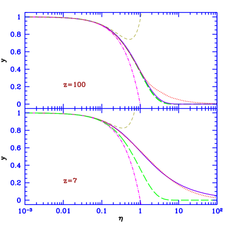
Figure 2: $y$ versus $\eta$ for two redshifts, $z=100$ (top panel) and $z=7$ (bottom panel). We compare the exact numerical results (dotted curves) to several approximations: the formula of equation (15) (solid curves), the redshift-independent first-order approximation (dot-dashed curves), the second-order approximation (short-dashed curves), and the redshift-independent exponential approximation (long-dashed curves) suggested by Gnedin et al. (2003) for the post-reionization regime.

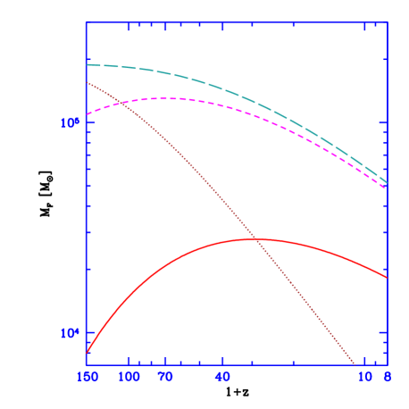
Figure 3: The filtering mass versus redshift. The exact calculation (solid curve), which can be fitted by equations (17) and (18), is compared to a couple versions of the mean sound speed approximation (see Sections 2.5 and 2.6): where the integrals in equation (25) are begun at time zero as written (long-dashed curve), or at cosmic recombination (short-dashed curve). Also shown is the Jeans mass (dotted curve), which is constant at $z\ga 150$.

We define the filtering mass in terms of the filtering wavenumber using the traditional convention used to define the Jeans mass:

$$M_{F}=\frac{4\pi}{3}\bar{\rho_{0}}\left(\frac{1}{2}\frac{2\pi}{k_{F}}\right)^{3}\ .$$ (16)

Note that this relation, which we use consistently in this paper, is one eighth of the definition in Gnedin (2000). The filtering mass essentially describes the largest mass scale on which pressure must be taken into account. Thus, in comparing different scenarios, those with higher gas temperatures will tend to have higher pressures, leading to higher values of the filtering mass.

Figure 3 shows the evolution of the filtering mass with redshift. Since the baryon fluctuations are very small before cosmic recombination, the gas pressure (which depends on $\delta_{b}$) is small compared to gravity (which depends on $\delta_{\mathrm{tot}}$; see equations (1)). Thus, the filtering mass starts from low values and rises with time at $z\sim 100$. At lower redshifts the gas cools and the pressure drops. Therefore, even at $z\sim 10$ the integral in equation (2.3) receives a large contribution from much higher redshifts ($z>100$).

We have found a simple, accurate fit for the evolution of the filtering mass in the redshift range of $z=7-150$. Using the notation $L_{M}\equiv\log(M_{F}/M_{\odot})$ and $L_{z}\equiv\log(1+z)$, the fit is of the form

$$L_{M}=\beta_{1}(\Omega_{m})L_{z}^{3}+\beta_{2}(\Omega_{m})L_{z}^{2}+\beta_{3}(\Omega_{m})L_{z}+\beta_{4}(\Omega_{m}).$$ (17)

The fitted coefficients are

$$\beta_{1}(\Omega_{m}) = -0.38\,\Omega_{m}^{2}+0.41\,\Omega_{m}-0.16\ ,$$ (18)

$$\beta_{2}(\Omega_{m}) = 3.3\,\Omega_{m}^{2}-3.38\,\Omega_{m}+1.15\ ,$$

$$\beta_{3}(\Omega_{m}) = -9.64\,\Omega_{m}^{2}+9.75\,\Omega_{m}-2.37\ ,$$

$$\beta_{4}(\Omega_{m}) = 9.8\,\Omega_{m}^{2}-10.68\,\Omega_{m}+11.6\ ,$$

where the maximum residual error of the fit is $0.2\%$, over the range $\Omega_{m}=$0.25–0.4 in $\Lambda$CDM.

2.4 Small Scale, Large-$k$ Limit

In this limit the pressure dominates and makes $\delta_{b}\ll[\delta_{\mathrm{tot}},\delta_{\mathrm{dm}}]$, and therefore the first equation (1) becomes:

$$\ddot{\delta}_{\mathrm{dm}}+2H\dot{\delta}_{\mathrm{dm}}\cong f_{\mathrm{dm}}\frac{3}{2}H_{0}^{2}\frac{\Omega_{m}}{a^{3}}\delta_{\mathrm{dm}}\ .$$ (19)

Equation (19) has a simple analytical solution in the EdS regime: $\delta_{\mathrm{dm}}\propto t^{\alpha}$, where $\alpha=\left(-1\pm\sqrt{1+24f_{\mathrm{dm}}}\right)/6$. In particular, the growing mode of the dark matter is reduced compared to the usual $\delta_{\mathrm{dm}}\propto t^{2/3}$ solution, since while the baryons contribute to the cosmic expansion rate (in the Friedmann equation) they do not, on small scales, contribute to perturbation growth. Thus, since the dark matter fluctuations on large scales grow by a factor of $\sim 300$ between recombination and $z=10$, then for $f_{\mathrm{dm}}=0.84$ the total growth of the dark matter fluctuations is reduced on small scales by a factor of $\sim 1.8$ relative to large scales. This linear calculation is limited to redshifts $\ga 10$, since even without reionization, by $z=10$ the filtering scale becomes non-linear.

2.5 Mean Sound Speed Approximation

Naoz & Barkana (2005) showed that the presence of spatial fluctuations in the sound speed modifies the calculation of perturbation growth significantly. Nevertheless, for completeness and ease of comparison with previous results we compare the above analysis to earlier, approximate calculations. Thus, we proceed by applying a similar derivation as in the previous sections. In this approximation of a uniform sound speed, however, the evolution of the density fluctuations is described by a different set of coupled second order differential equations:

$$\ddot{\delta}_{\mathrm{dm}}+2H\dot{\delta}_{\mathrm{dm}} = \frac{3}{2}H_{0}^{2}\frac{\Omega_{m}}{a^{3}}\left(f_{\mathrm{b}}\delta_{\mathrm{b}}+f_{\mathrm{dm}}\delta_{\mathrm{dm}}\right)\ ,$$ (20)

$$\ddot{\delta}_{\mathrm{b}}+2H\dot{\delta}_{\mathrm{b}} = \frac{3}{2}H_{0}^{2}\frac{\Omega_{m}}{a^{3}}\left(f_{\mathrm{b}}\delta_{\mathrm{b}}+f_{\mathrm{dm}}\delta_{\mathrm{dm}}\right)-\frac{k^{2}}{a^{2}}c^{2}_{s}\delta_{\mathrm{b}}\ ,$$

where $c_{s}^{2}=dp/d\rho$ is assumed to be spatially uniform (i.e., independent of $k$). With this assumption, the temperature fluctuations (as a function of $k$) are simply proportional at any given time to the gas density fluctuations:

$$\frac{\delta_{T}}{\delta_{\mathrm{b}}}=\frac{c_{s}^{2}}{k_{B}\bar{T}/\mu}-1\ .$$ (21)

This leads to different expressions for the filtering mass.

2.6 Mean Sound Speed Approximation: The Filtering Scale

We again expand the ratio of the baryon fluctuations to dark matter fluctuations in powers of $k^{2}$. In this case we follow the derivation in Gnedin & Hui (1998) and thus make several additional assumptions: that the baryon fraction is small $(f_{\mathrm{b}}\ll f_{\mathrm{dm}})$, that the dark matter perturbation growth is dominated by the growing mode ($\delta_{\mathrm{dm}}\propto D_{+}$), and that there is no initial difference between the baryon and the dark matter fluctuations. Although this derivation includes several different approximations, for simplicity we refer to it as the “mean sound speed approximation”. With these assumptions,

$$\frac{\delta_{\mathrm{b}}}{\delta_{\mathrm{dm}}}=1-\frac{k^{2}}{k_{F,c_{s}}^{2}}\ .$$ (22)

Writing this as

$$k^{2}_{F,c_{s}}(t)=\frac{\delta_{\mathrm{dm}}(t)}{u_{c_{s}}(t)}\ ,$$ (23)

and substituting into equations (20), we obtain an equation for the evolution of the parameter $u_{c_{s}}$ (analogous to equation (11)):

$$\ddot{u}_{c_{s}}+2H\dot{u}_{c_{s}}=\frac{c_{s}^{2}}{a^{2}}D_{+}(t)\ .$$ (24)

The solution (in analogy with equation (2.3)) is

$$u_{c_{s}}(t)=\int^{t}_{0}\frac{dt^{\prime\prime}}{a^{2}(t^{\prime\prime})}\int_{0}^{t^{\prime\prime}}dt^{\prime}c^{2}_{s}(t^{\prime})D_{+}(t^{\prime})\ .$$ (25)

We note that the lower limit of the integral here is $z\to\infty$, and not recombination as in equation (2.3). Before recombination, the coupling of the baryons with the radiation suppresses the baryon density fluctuations, but this is unaccounted for in this approximate calculation. Indeed, this formula implicitly assumes that the baryon perturbations grow like those of the dark matter, except for the effect of pressure. In particular, the filtering scale in this approximation does not depend on the relative contributions of the baryons and the dark matter to the total matter density.

In Figure 3, we show the filtering mass with this approximation from Gnedin & Hui (1998). The correct filtering mass at $z\sim 10$ is substantially lower than predicted by the mean sound speed approximation. As noted before, this is mainly due to the fact that pressure forces depend on gradients in the gas density, and the baryon perturbations are reduced on all scales until they catch up with the dark matter fluctuations (at $z\ll 100$). In the approximate model, on the other hand, the initial difference between the baryon and the dark matter fluctuations is incorrectly neglected.

In the Figure, we consider also the mean sound speed approximation where we start the integral in equation (25) at recombination ($z=1200$). This should be more realistic than starting at time zero, since the baryon density fluctuation before recombination were negligible. This causes a rise in the filtering mass at $z\sim 100$, as in the correct calculation (i.e., the solid curve). However, the rise at high redshift is still much too fast, since this approximation still assumes that the baryons catch up with the dark matter fluctuations immediately after recombination.

To summarize, the Figure shows that the difference between the the correct calculation and the approximate one persists with time. This difference is remembered through the integrated effect of pressure, since at low redshift the Jeans mass is lower and thus the pressure is lower as well. Therefore, the high redshifts contribute most to the integrated pressure, and thus even though the difference between the baryon and the dark matter fluctuations declines with time (e.g., see Figure 1 top panel), the system still remembers the initial difference.

2.7 Gas Fraction

One useful application of the filtering mass is to the estimation of the fraction of gas inside halos. Gnedin (2000, his equation (8)) estimated the mean baryonic mass $M_{g}$ in halos of total mass $M_{\mathrm{tot}}$ using a formula fitted to his post-reionization simulation:

$$\bar{M}_{g}(M_{\mathrm{tot}},t)\approx\frac{f_{\mathrm{b}}M_{\mathrm{tot}}}{\left[1+(2^{1/3}-1)M_{c}(t)/M_{\mathrm{tot}}\right]^{3}}\ ,$$ (26)

where $M_{c}(t)$ is a characteristic halo mass that corresponds to a gas fraction of $50\%$ of the cosmic baryon fraction. It is natural to expect a close relation between the characteristic halo mass and the filtering mass, since the gas fraction in a collapsing halo reflects the amount of gas that was able to accumulate in the central, collapsing region, during the entire extended collapse process. In particular, if the Jeans mass changes suddenly, this does not immediately affect then-collapsing halos. A change of pressure immediately begins to affect gas motions (through the pressure-gradient force), but has only a gradual, time-integrated effect on the overall amount of gas in a given region.

As mentioned before, our definition of the filtering mass (equation (16)) is one eighth of the previous definition of Gnedin (2000). Thus the characteristic mass that matches the Gnedin (2000) simulations corresponds to about 8 times our filtering mass. Assuming that this is true also prior to reionization, we can evaluate the total gas fraction in halos as a function of redshift as

$$F_{g}(z)=\int{f_{ST}(M_{\mathrm{tot}},z)\,\frac{\bar{M}_{g}(M_{\mathrm{tot}},t)}{M_{\mathrm{tot}}}\,dS}\ ,$$ (27)

where $S=\sigma^{2}(M,z)$ is the variance and $f_{ST}$ is the Sheth & Tormen (2001) function for the fraction of mass associated with halos of mass $M$ (explicitly given in equation (33), below).

The total fraction of gas that is in halos is shown in Figure 4, for our correct calculation of the filtering mass as well as for the previous calculation (which we have referred to as the mean sound speed approximation). We also compare to the fraction of gas in halos above the minimum $H_{2}$ cooling mass, and to the fraction above the minimum atomic cooling mass. In the correct calculation, a significant part (10–$50\%$) of the total gas in halos arises from halos that are below the characteristic mass. The prediction of the gas fraction in halos in our correct calculation is higher than that based on the previous approximation, by a factor $>2$ at high redshifts and still by $10\%$ at redshift 7. In this redshift range, around half the gas in halos is in potentially star-forming halos (i.e., those with efficient $H_{2}$ cooling), and the rest is in gas minihalos. In particular, this means that the smallest star-forming halos (i.e., those with a mass equal to the minimum $H_{2}$ cooling mass) are moderately affected by pressure, and have their gas content reduced to around half the cosmic baryon ratio.

The importance of the pressure in halos of mass equal to the minimum H₂ cooling mass is illustrated in Figure 5. We consider the improved calculation (solid curve) and the mean sound speed approximation (short-dashed curve). This Figure shows that for the very first stars the previous calculation underestimates the gas fraction in these halos by more than an order of magnitude. E.g., at $1+z=66$ (the formation of the first star) the improved calculation predicts that the gas is about $35\%$ of the cosmic baryon fraction in halos with mass equal to the H₂ cooling mass, while the mean sound speed approximation predicts only $1.3\%$. Thus, we conclude that the effect of pressure on the very first stars is only moderate, unlike the result suggested by the mean sound speed approximation. The discrepancy decreases with the redshift. However, at $1+z=20$ the previous calculation still underestimates the gas fraction by a factor of 2, and even at $1+z=8$ the previous calculation underestimates the gas fraction by about $10\%$ compared with the improved calculation.

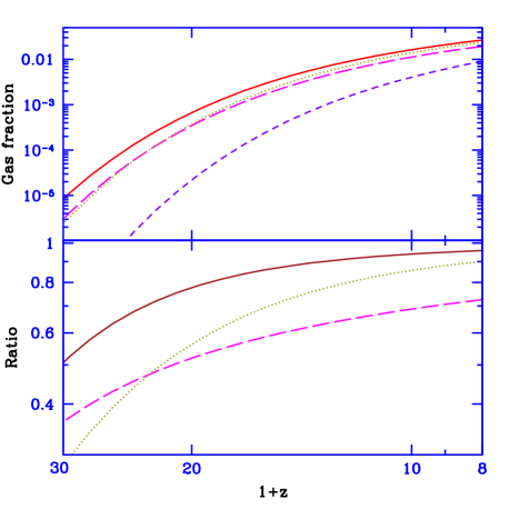
Figure 4: Top panel: Gas fraction in halos versus redshift. We show our correct calculation (solid curve) and the previous calculation using the filtering mass in the mean sound speed approximation (dotted curve). We also compare to the fraction of gas in halos above the $H_{2}$ cooling mass (long-dashed curve), and the fraction above the atomic cooling mass (short-dashed curve). Bottom panel: Ratio of gas fractions in different cases. We consider the gas fraction in halos above the characteristic mass (solid curve), the gas fraction in halos above the $H_{2}$ cooling mass (long-dashed curve), and the gas fraction in the mean sound speed approximation (dotted curve); each is divided by the total gas fraction in halos in our correct calculation.

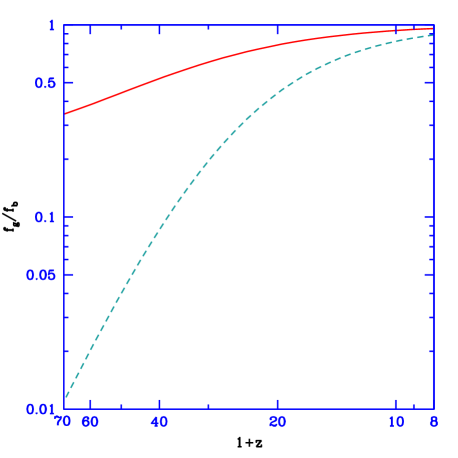
Figure 5: The gas fraction in halos of mass equal to the minimum H₂ cooling mass compared to the cosmic fraction. We plot the improved calculation (solid curve) and the mean sound speed approximation (short-dashed curve). In the latter case we have used the previous estimate, starting the integrals in eq. (25) at $t=0$.

3 Formation of Non-Linear Objects

The small amplitude density fluctuations probed by the CMB grow over time as described by equations (1) and (2), as long as the perturbations are linear. However, when $\delta$ in some region becomes of order unity, the full non-linear problem must be considered. The standard calculation that describes the formation of spherical non-linear objects was done for a dark matter halo only, as was explained in Section 1. Here, we generalize the calculation to the high-redshift regime, including the gravitational effects of the baryons and the radiation.

The initial conditions in N-body simulations of the first galaxies are set long after the recombination epoch (usually at $z\sim 200$ or later). Halos that collapse early ($z\sim 20$ and earlier) thus cannot arise from fluctuations that are linear at the beginning of the simulation, regardless of the size of the corresponding perturbed region. Now, perturbations that correspond to galaxies or clusters start from a comoving length below 100 Mpc and are thus expected to have entered the horizon at some time $t_{enter}$ in the radiation dominated era. The perturbations then do not grow significantly until equality ($z\sim 3000$). If we follow the evolution of a collapsing halo, then the linear $\delta$ grows approximately $\propto a$ after equality. Thus a region that collapses to a halo at $z\sim 100$ must have entered equality already in the weakly non-linear regime ($\delta\sim 1.686/30\sim 5\%$); since growth was slow before then, even when the halo entered the horizon in the radiation dominated universe, the perturbation was not extremely small. In practical applications, we find that the largest $\delta$ gets at horizon crossing is $\sim 10^{-3}$, for halos hosting the very first stars (Naoz, Noter & Barkana, 2006), so that non-linear corrections are always small. For completeness, however, we first consider the behavior of spherical fluctuations outside the horizon.

3.1 Fluctuation Growth Outside the Horizon

We consider a spherical top-hat fluctuation bigger than the Hubble radius at an early cosmic time. Since the fluctuation is outside the horizon, we cannot use Newtonian perturbation theory, and must apply General Relativity.

We consider a spherical overdensity with a uniform density $\rho=\bar{\rho}\left(1+\delta\right)$. Birkhoff’s theorem implies that the Friedmann equation is the correct solution within the spherical region (which has a curvature $\tilde{k}$):

$$H_{sph}^{2}=H_{0}^{2}\left[\frac{\Omega_{m}}{a^{3}}\left(1+\delta\right)+\frac{\Omega_{r}}{a^{4}}\left(1+\delta\right)^{\frac{4}{3}}+\frac{\Omega_{\tilde{k}}}{a_{sph}^{2}}+\Omega_{\Lambda}\right]\ ,$$ (28)

where $H_{sph}$ and $a_{sph}$ are the Hubble constant and expansion parameter, respectively, associated with the evolution of the perturbed region, while $a$ describes the cosmic expansion of the mean universe. The $4/3$ power is a result of the difference between the non-relativistic (dark matter and baryon) density fluctuation $\delta$ and the radiation density fluctuation.

Just as in the regular top-hat collapse, we wish to compare the exact non-linear evolution (given by equation (28)) to the linearly-extrapolated evolution. Comparing the above non-linear equation to the evolution of the background universe and linearizing, we obtain:

$$2H\alpha\dot{\delta}=I^{2}\delta-\frac{\tilde{k}}{a^{2}},$$ (29)

where $I^{2}=H_{0}^{2}[\Omega_{m}/a^{3}+(4/3)\Omega_{r}/a^{4}]$, and $\alpha=0.5\,I^{2}/\dot{H}$; at high redshift, in the radiation-dominated regime, $\alpha\approx-0.25$ and then $\delta\propto a^{2}$ (corresponding to the synchronous gauge; Ma & Bertschinger (1995); Padmanabhan (2002)). We start early enough so that $\delta=1\times 10^{-4}$ initially, and assume the growing mode for the initial perturbation. Solving numerically the non-linear and linear equations (equations (28) and (29)), until the fluctuation enters the horizon, yields the initial value of the fluctuation entering the horizon in the radiation dominated universe. As noted above, in practice, linear initial conditions at horizon crossing would suffice for the parameter space we consider in this paper.

3.2 Fluctuation Growth Inside the Horizon

In the Newtonian regime the non-linear growth is described by the Newtonian equation (or, more precisely, the equation for the acceleration that results from the Einstein equations):

$$\ddot{r}=-\frac{GM}{r^{2}}-\frac{4\pi G}{3}\left(\rho+3P\right)_{rest}r\ ,$$ (30)

where the rest stands for all matter that does not participate in the collapse, and thus only contributes to the expansion of the universe. We define $r_{\mathrm{dm}}$ and $r_{\mathrm{b}}$ to be physical radii that enclose a fixed mass of dark matter and of baryons, respectively, assuming a tophat perturbation in each. Then we obtain two coupled non-linear equations of motion:

$$\ddot{r}_{\mathrm{dm}} = \frac{-1}{r^{2}_{\mathrm{dm}}}\frac{4\pi G}{3}r_{\mathrm{dm}}^{3}\left(\rho_{\mathrm{dm}}+\rho_{\mathrm{b}}\right)+H_{0}^{2}\Omega_{\Lambda}r_{\mathrm{dm}}-\frac{8\pi G}{3}\rho_{r}r_{\mathrm{dm}}\ ,$$

$$\ddot{r}_{\mathrm{b}} = \frac{-1}{r^{2}_{\mathrm{b}}}\frac{4\pi G}{3}r_{\mathrm{b}}^{3}\left(\rho_{\mathrm{dm}}+\rho_{\mathrm{b}}\right)+H_{0}^{2}\Omega_{\Lambda}r_{\mathrm{b}}-\frac{8\pi G}{3}\rho_{r}r_{\mathrm{b}}\ .$$ (31)

We have assumed that the radiation is kept smooth by its own pressure and does not participate in the collapse; the factor $8\pi/3$ is the result of inserting $P_{r}=\rho_{r}/3$ in equation (30). Since the time when the fluctuation enters the horizon is substantially early in the radiation-dominated universe, the baryon-photon coupling yields $\delta_{\mathrm{b}},\delta_{\gamma}\ll\delta_{\mathrm{dm}},\delta_{\mathrm{tot}}$ initially. We calculate separately the linear and non-linear growth of the fluctuations. The resulting critical (linear) overdensity at the time of collapse is shown in Figure 6. For the cosmological parameters that we use in this paper, we find that $\delta_{c}$ is essentially independent of $M$, and is lower than the EdS value by $\sim 1\%\times(1+z)/20$ in the range of $z=9-100$. When dealing with very rare halos, even a change of a few percent in $\delta_{c}$ can change the halo abundance at a given redshift by over an order of magnitude (see Figure 2 of Naoz, Noter & Barkana (2006)). The results are insensitive to the cosmological parameters: also shown in Figure 6 are the results for the set of other parameters (Section 1) specified by Viel et al. (2006), which differ by 1-$\sigma$ from our standard WMAP parameters; the results are almost identical in the EdS regime ($1+z=2-10$), with only a $\la 0.2\%$ difference at high redshift (and even less at $z<1$).

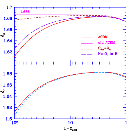
Figure 6: Critical overdensity versus collapse redshift. We compare $\delta_{c}$ for the full calculation (solid curves) to the results with other assumptions. The top panel compares to several cases that include only some of the physical ingredients that affect the spherical collapse calculation. We show the results of previous calculations that did not properly include the baryons and photons at high redshift (dotted curve), the results if the baryons are treated correctly but the contribution of the uniform radiation background is neglected (long-dashed curve), and the results if the radiation is included but the baryon-photon coupling is neglected (i.e., the baryons are treated like dark matter: short-dashed curve). The bottom panel shows results also for the Viel et al. (2006) set of parameters (dashed curve).

The effect of various physical ingredients on $\delta_{c}$ can be illustrated using the different cases shown in the upper panel of Figure 6. In general, collapse is most efficient in the EdS case where all the matter participates in the collapse (resulting in $\delta_{c}=1.686$); any smooth component that does not collapse (a cosmological constant at low redshift, radiation and baryons at high redshift) reduces the collapse efficiency since only the dark matter component takes part in the collapse throughout. Now, any reduction in the matter fraction that collapses depresses the linear evolution of the density perturbation more strongly, while the non-linear perturbation is larger and is thus less affected by the components that do not help in the collapse. Therefore the linear perturbation reaches a lower value of $\delta_{c}$ when the non-linear perturbation collapses. As shown in the upper panel of Figure 6, the extended period at high redshift when the baryon perturbations remain suppressed is the main cause of the reduction of the value of $\delta_{c}$, but the contribution of the photons to the expansion of the universe also makes a significant contribution.

3.3 The Mass Function and Halo Abundance

In addition to characterizing the properties of individual halos, it is important for any model of structure formation to predict also the abundance of halos. We calculate in this section the number density of halos as a function of mass, at any redshift. We start with the simple analytical model of Press & Schechter (1974), which is based on Gaussian random fields, linear growth and spherical collapse. It predicts that the abundance of halos depends on mass and redshift through the two functions $\sigma(M,z)$ and $\delta_{c}(z)$, where $\sigma^{2}(M,z)$ is the variance (calculated from the power spectrum) as a function of halo mass at $z$, and $\delta_{c}(z)$ is the critical collapse overdensity from Section 3.2.

In Figure 7 we show the number of $\sigma$ that a fluctuation must be in order for it to collapse, at various redshifts from the first star until the present. For example, a $10^{5}M_{\odot}$ halo that collapses and forms the first star is a 9.5-$\sigma$ fluctuation according to this criterion (but see below). Halos of mass $10^{5}M_{\odot}$ become 1-$\sigma$ fluctuations only at $z\sim 5$, while today the 1-$\sigma$ collapsing fluctuations are $10^{13}M_{\odot}$ group halos.

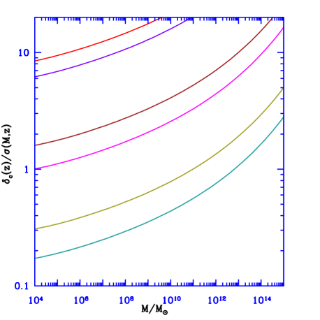
Figure 7: Rarity of fluctuations that produce halos at various redshifts. We show the size of a fluctuation that produces a collapsed halo on the scale $M$ at redshift $z$, in terms of the typical fluctuation level (i.e., measured as a number of $\sigma$). This includes $\sigma(M,z)$ from the correct calculation of the power spectrum (Naoz & Barkana, 2005), and $\delta_{c}(z)$ from the correct spherical collapse calculation (Section 3.2). We consider, from bottom to top, $z=0$, 1.2, 6.5, 11, 47 and 66. Redshift 66 corresponds to the formation of the first star, while $z=47$ corresponds to the redshift of the second generation of stars, i.e., the first collapse via atomic cooling. Redshift 11 corresponds to the first halo as massive as that of the Milky Way and $z=1.2$ is associated with the formation of the first cluster as massive as Coma (see Naoz, Noter & Barkana (2006)). We also show the results at $z=6.5$ associated with observations of the most distant quasars (and perhaps with the end of reionization).

The growth of the density fluctuations in our correct calculation can be described by an effective growth factor which depends on the mass scale: $D_{\rm eff}\equiv\sigma(M,z)/\sigma(M,z=0)$. We compare this effective growth factor to the traditional growing mode $D(z)$ (Peebles, 1980) in Figure 8, where we show $D_{\rm eff}/D-1$ as a function of mass, illustrated at the same redshifts as in Figure 7. The source of the difference is in the smoothness of the radiation and baryons at high redshifts; in addition, pressure suppresses growth on small mass scales. These effects make $D_{\rm eff}$ larger at high redshift compared to its value today (since there has been less growth).

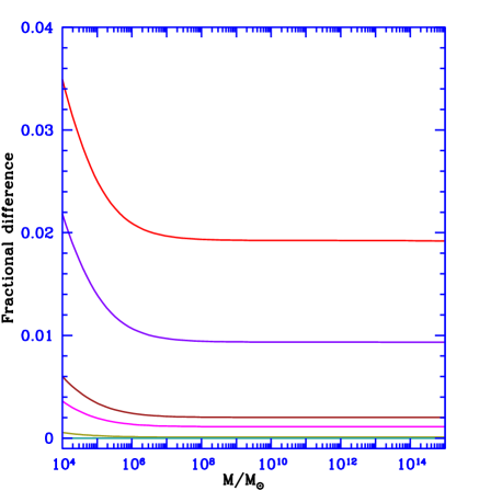
Figure 8: The fractional difference between the effective growth factor of our correct calculation, $\sigma(M,z)/\sigma(M,z=0)$, and the traditional growth factor $D(z)$, as a function of mass at various redshifts. We consider, from bottom to top, $z=0$, 1.2, 6.5, 11, 47 and 66, as in Figure 7.

The comoving number density of halos of mass $M$ at redshift $z$ is

$$\frac{dn}{dM}=\frac{\rho_{0}}{M}f_{ST}\left|\frac{dS}{dM}\right|\ ,$$ (32)

were we have used the Sheth & Tormen (2001) mass function that fits simulations, and includes non-spherical effects on the collapse. The function $f_{ST}$ is the fraction of mass associated with halos of mass $M$:

$$f_{ST}(\delta_{c},S)=A^{\prime}\frac{\nu}{S}\sqrt{\frac{a^{\prime}}{2\pi}}\left[1+\frac{1}{\left(a^{\prime}\nu^{2}\right)^{q^{\prime}}}\right]\exp\left[\frac{-a^{\prime}\nu^{2}}{2}\right]\ ,$$ (33)

where $\nu=\delta_{c}/\sqrt{S}$. We use best-fit parameters $a^{\prime}=0.75$ and $q^{\prime}=0.3$ (Sheth & Tormen, 2002), and ensure normalization to unity by taking $A^{\prime}=0.322$. We apply this formula with $\delta_{c}(z)$ and $\sigma^{2}(M,z)$ as the arguments. The Sheth & Tormen (2001) mass function makes it easier for rare fluctuations to collapse compared to Press & Schechter (1974). This, for instance, makes the first star-forming halo effectively only an 8.3-$\sigma$ density fluctuation on the mass scale of $10^{5}M_{\odot}$, in terms of the total cosmic mass fraction contained in halos above this mass.

The cumulative comoving number density of halos $n(>M_{\rm min})$ is given by

$$n(>M_{\rm min})=\int_{M_{\rm min}}^{\infty}\frac{dn}{dM}\,dM\ .$$ (34)

In Figure 9 we plot the cumulative number density of halos. In addition to our standard WMAP cosmological parameter set, we have also compared to the Viel et al. (2006) set of parameters (Section 1). We obtained for these parameters that the first star formed at $z=60.0$ (instead of 65.8) and the first Coma size cluster formed at $z=1.06$ (instead of 1.24). The difference between the two sets of cosmological parameter arises mainly from the difference in $\sigma_{8}$. The difference in the values of $\delta_{c}$ is negligible (see Figure 6).

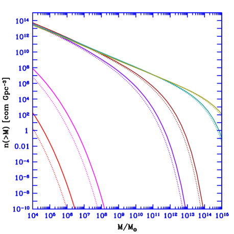
Figure 9: The halo abundance as a function of the halo mass at different redshifts. From top to bottom (at the high-mass end): $z=0,1.2,6.5,11,47$ and finally $z=66$ which corresponds to the formation of the first star (Naoz, Noter & Barkana, 2006). We consider our standard WMAP cosmological parameters (solid curves), and compare to the Viel et al. (2006) set of parameters (dotted curves).

4 Conclusions

We have calculated the filtering mass correctly at high redshift and compared it to previous estimates. We have found that at high redshift the filtering mass is lower by about an order of magnitude compared to previous calculations. The difference declines with time but remains a factor of $\sim 3$ even at $z=7$ (Figure 3). Our calculation predicts a lower filtering mass because it includes the initial difference between the dark matter and baryon fluctuations, due to the baryon-photon coupling, and this lowers the pressure. This means that in contrast with the previous prediction, pressure has only a moderate effect on the formation of the earliest luminous objects.

Before recombination the baryon fluctuations were suppressed compared to the dark matter fluctuations due to tight coupling with the radiation. The filtering mass rises with time at high redshift because after recombination the baryon pressure gradients start to increase. However, after the baryon temperature decouples from the CMB temperature the gas cools adiabatically, the Jeans mass drops, and eventually (at lower redshifts) the filtering mass drops as well (see Figure 3). The high pressure at very high redshift still contributes significantly to the filtering mass at redshift below 10. The delay in the drop of the filtering mass compared to the Jeans mass is a signature of the continuing contribution of the memory of the pressure from very high redshifts. We have found numerical fits to the difference between the baryon and the total density fluctuations on large scales (equations (6)); we have also fit the filtering mass as a function of $\Omega_{m}$ and $z$ (equations (17) and (18)).

Using the new prediction of the filtering mass we have shown that at high redshift there is more gas in halos than in previous estimates. This difference is as large as a factor of 2, but remains $\sim 10\%$ even at redshift 7. Around half of the gas is in halos with efficient $H_{2}$ cooling, and the rest is in gas minihalos. The previous calculation also suggests a greatly reduced gas fraction in the halo that hosts the first star, while we find only a moderate effect (Figure 5).

In addition, we have computed the evolution of linear as well as non-linear spherical overdensities, outside and inside the horizon, in a $\Lambda$CDM universe. Previous analyses showed that the cosmological constant contribution to the expansion of the universe results in a drop of the value of $\delta_{c}$ by $\sim 0.6\%$ today (e.g., Lahav et al., 1991). This makes a significant difference in the abundance of clusters. Considering structure formation at high redshift, we investigated the effect on $\delta_{c}$ and on the halo abundance of the contribution of radiation to the expansion of the universe, and of the contribution of the baryons to the collapsing halo, given their different initial conditions compared to the dark matter. We have found that there is a $3\%$ change in the value of the overdensity $\delta_{c}$ at $z\sim 60$ (Figure 6). This changed value translates to a much larger difference in the halo abundance at high redshift (Figure 9); these differences decline at low redshift. The large difference in the halo abundance is the result of the difference in the exponent in the mass function (equation (33)), and shows that even small effects on halo formation can in some cases be very important.

References

- Abel et al. (2002) Abel T., Bryan G. L., Norman M. L., 2002, Sci, 295, 93
- Barkana & Loeb (2001) Barkana R., Loeb A., 2001, PhR, 349, 125
- Barkana & Loeb (2005) Barkana R., Loeb A., 2005, MNRAS, 363, L36
- Barkana (2006) Barkana R., 2006, Sci, 313, 931
- Bennett et al. (1996) Bennett C. L., et al., 1996, ApJ, 464, 1
- Deshingkar et al. (2001) Deshingkar S. S., Jhingan S., Chamorro A., Joshi P. S., 2001, PhRvD, 63, 124005
- Fuller (2000) Fuller T. M., Couchman H. M. P., 2000, ApJ, 544, 6
- Gnedin & Hui (1998) Gnedin N. Y., Hui, L., 1998, MNRAS, 296, 44
- Gnedin (2000) Gnedin N. Y., 2000, ApJ, 542, 535
- Gnedin et al. (2003) Gnedin N. Y., et al., 2003, ApJ, 583, 525
- Gunn & Gott (1972) Gunn J. E., Gott J. R., 1972, ApJ, 176, 1
- Haiman et al. (1997) Haiman Z., Rees M. J., Loeb A., 1997, ApJ, 476, 458
- Horellou & Berge (2005) Horellou C., Berge J., 2005, MNRAS, 360, 1393
- Kashlinsky et al. (2005) Kashlinsky, A., Arendt, R. G., Mather J., Moseley S. H., 2005, Natur, 438, 45
- Lahav et al. (1991) Lahav O., Lilje P. B., Primack J. R., Rees M. J., 1991, MNRAS, 251, 128
- Lokas & Hoffman (2001) Lokas E. L., Hoffman Y., 2001, Proc. 3rd Int. Workshop on the Identification of Dark Matter, World Scientific, Singapore, p. 121
- Ma & Bertschinger (1995) Ma C., Bertschinger E., 1995, ApJ, 455, 7
- Maor & Lahav (2005) Maor I., Lahav O., 2005, MNRAS, 7, 3
- Naoz & Barkana (2005) Naoz S., Barkana R., 2005, MNRAS, 362, 1047
- Naoz, Noter & Barkana (2006) Naoz S., Noter S., Barkana R., 2006, MNRAS, 373, L98
- Ostriker & Steinhardt (2003) Ostriker J. P., Steinhardt P., 2003, Sci, 300, 1909
- Padmanabhan (2002) Padmanabhan T., 2002, Theoretical Astrophysics, Volume III: Galaxies and Cosmology, Cambridge Univ. Press, Cambridge, UK.
- Peebles (1980) Peebles P. J. E., 1980, The Large-Scale Structure of the Universe, Princeton Univ. Press, Princeton
- Press & Schechter (1974) Press W. H., Schechter P., 1974, ApJ, 187, 425
- Riess et al. (1998) Riess A. G., et al., 1998, AJ, 116, 1009
- Sheth & Tormen (2001) Sheth R. K., Mo H. J., Tormen G., 2001 ,MNRAS, 323, 1
- Sheth & Tormen (2002) Sheth R. K., Tormen G., 2002, MNRAS, 329, 61
- Spergel et al. (2003) Spergel D. N., et al., 2003, ApJ, 148, 175
- Spergel et al. (2006) Spergel D. N., et al., 2006, astro-ph/0603449
- Tegmark (1997) Tegmark M., et al., 1997, ApJ, 474, L77
- Viel et al. (2006) Viel M., Haehnelt M. G., Lewis, A., 2006, MNRAS, 370, L51
- Wang (2005) Wang, P., 2005, astro-ph/0507195
- Yoshida (2005) Yoshida N., 2005, PThPS, 158, 117