Neutralino Dark Matter and the Curvaton

Abstract

We build a realistic model of curvaton cosmology, in which the energy content is described by radiation, WIMP dark matter and a curvaton component. We calculate the curvature and isocurvature perturbations, allowing for arbitrary initial density perturbations in all fluids, following all species and their perturbations from the onset of dark matter freeze-out onto well after curvaton decay. We provide detailed numerical evaluations as well as analytical formulae which agree well with the latter. We find that substantial isocurvature perturbations, as measured relatively to the total curvature perturbation, can be produced even if the curvaton energy density is well underdominant when it decays; high precision measurements of cosmic microwave background anisotropies may thus open a window on underdominant decoupled species in the pre-nucleosynthesis early Universe. We also find that in a large part of parameter space, curvaton decay produces enough dark matter particles to restore WIMP annihilations, leading to the partial erasure of any pre-existing dark matter - radiation isocurvature perturbation.

I Introduction

According to standard lore, the cosmological density perturbations at the origin of large scale structure were seeded at some very early time by the decay of the field that is also responsible for inflation. In the past few years, there has been growing interest in a variant of this cosmological scenario, in which another field, denoted the “curvaton”, communicates its own perturbations to matter and radiation. In the simplest version, the curvaton plays a negligible rôle in determining the dynamics of the Universe at the time of inflation, but comes to dominate the energy density in the radiation era, and as such, it becomes the seed of energy density perturbations through its decay. From a technical point of view, the curvaton scenario transforms an initially isocurvature perturbation into an adiabatic (or curvature) perturbation, as demonstrated in another context in Ref. [1] and more recently in Ref. [2] (see also Ref. [3]).

In the “simplest” curvaton model, radiation is composed of a single fluid deprived of an intrinsic density perturbation before curvaton decay; the final perturbation is then purely adiabatic. However, as already noted in [2], radiation is generically a mixture of different interacting fluids, so that if the curvaton decays after the decoupling of one of the constituents, an isocurvature perturbation will appear between this latter and the rest of radiation. Detailed calculations have been provided in Refs. [6, 7] for isocurvature perturbations generated between photons and baryons, between photons and neutrinos as well as between photons and dark matter and their impact on the CMB anisotropies. Non-gaussian signatures are also to be expected [8, 9]. The implementation of a curvaton scenario in the framework of high energy physics and supersymmetric theories has been proposed in several studies, see for instance [10].

Since any pre-existing isocurvature perturbation between two interacting fluids is erased on a short timescale if the fluids share thermal equilibrium [11], an isocurvature perturbation can only be generated when the curvaton decays after the decoupling of one of these components. In this respect, the case of WIMP dark matter - photon isocurvature perturbation appears particularly interesting. Dark matter is indeed expected to decouple very early on from radiation, hence this leaves significant room for the curvaton to decay after decoupling and before big-bang nucleosynthesis (as required by cosmology). This may be put in contrast with baryons and neutrinos which decouple just before big-bang nucleosynthesis.

To our knowledge, there is no exhaustive survey of the curvature and isocurvature perturbations generated in a “realistic” curvaton model which takes into account the existence of radiation and dark matter, the influence of the freeze-out of this latter fluid, the influence of initial density perturbations in radiation and dark matter and the different decay widths of curvaton into radiation and dark matter. For instance, Ref. [6] has computed the isocurvature and curvature perturbations under specific assumptions on the origin of dark matter, neglecting the effect of freeze-out and of different branching ratios. The generation of a net isocurvature fluctuation during dark matter freeze-out consecutive to the presence of the curvaton has been computed in Ref. [9] but without discussing the evolution through curvaton decay. In [12], an initial density perturbation in the radiation fluid has been taken into account but the presence of dark matter was neglected. Ref. [13], building on the general formalism developed in [14], has considered a three-fluid model of curvaton decay, albeit assuming that dark matter fully originates in the decay of the curvaton. Finally, Ref. [15] has presented a detailed numerical evaluation of the curvature and isocurvature perturbations in a three-fluid model of curvaton decay and their impact on CMB anisotropies, without however specifying the origin of dark matter.

Our present objective is to make progress along these lines and to present a comprehensive model of curvaton - radiation and WIMP dark matter cosmology, building on the above earlier studies. We will present analytical and numerical calculations of the perturbations produced, following in detail the freeze-out of equilibrium of dark matter annihilations and curvaton decay, with non-vanishing initial perturbations in the radiation - dark matter sector and in the curvaton field. We focus on WIMP (neutralino) dark matter, since it offers at present one of the best motivated candidates for dark matter. It further allows one to set a specific framework for the thermal history of the different fluids, without having to rely on the details of the underlying particle physics models. The scenario, and its cosmological consequences, would certainly be different for axion like dark matter, whose scrutiny is postponed to future study.

The paper is arranged as follows. In the following section, i.e. Sec. II, we describe the three-fluid model and establish the equations of motion both at the background level, see Sec. II.1, and at the perturbed level, see Sec. II.2. In Sec. III, we solve these equations by approximate analytical methods. In Sec. IV, in order to assess the validity of our approximations, we investigate the evolution of the background and of the perturbations by means of numerical calculations. The physical interpretation of our results is also discussed at length in this section. Finally, in Sec. V, we present our conclusions. Some specific technical details are also presented in three appendices at the end of the paper. In App. A, we briefly recall how the gauge-invariant quantities relevant to the present work are defined and how their equations of motion can be derived. In App. B, we explain how to quantify the influence of the curvaton perturbations during freeze-out [our Eq. (22)] using junction conditions. In App. C, we provide an extended discussion of the theorem of Weinberg [11] on the approach to adiabaticity for the perturbations of interacting fluids in terms of gauge-invariant quantities.

II Detailed three-fluid model

We are interested in computing the curvature and isocurvature perturbations produced in a three-fluid model composed of radiation (denoted by the subscript $\gamma$ in what follows), a curvaton component (denoted $\sigma$) and dark matter (denoted by $\chi$). The dark matter particles share thermal equilibrium with radiation until their freeze-out of equilibrium after having turned non-relativistic. We denote by $x_{\rm f}$ the ratio of mass $m_{\chi}$ to temperature at which freeze-out occurs: $x_{\rm f}\equiv m_{\chi}/T_{\rm f}$. In the particular case of neutralino dark matter, one generically finds $x_{\rm f}\simeq 20$. Unless otherwise noted, we use $x_{\rm f}=20$ as a fiducial value in what follows.

We further assume that the curvaton is very weakly coupled to the visible sector (radiation + dark matter) and that it decays into this sector after dark matter freeze-out. Were it to decay earlier, there would be no final isocurvature perturbation between $\chi$ and $\gamma$, in virtue of the theorem of Weinberg on the approach to adiabaticity of interacting fluids [11]. This point is addressed with greater scrutiny in Appendix C, where it is shown, in particular, to be in excellent agreement with numerical computations. If the curvaton were to couple to the visible sector so that it had at some point shared thermal equilibrium, any pre-existing isocurvature perturbation between itself and radiation or dark matter would likewise have been erased. Hence the above assumption is one of non-triviality. It is furthermore consistent, in the sense that a late decay is a generic consequence of a very weak coupling; moduli fields, in particular, emerge as natural candidates in this curvaton scenario.

We denote by $\Gamma_{\sigma}$ the total decay width of the curvaton, $\Gamma_{\sigma\gamma}$ and $\Gamma_{\sigma\chi}$ its partial decay widths into radiation and dark matter, respectively. Decay of the curvaton occurs when $\Gamma_{\sigma}\approx H$, hence our previous assumption corresponds to $\Gamma_{\sigma}\ll\Gamma_{\chi\chi|\rm f}$, where the latter quantity $\Gamma_{\chi\chi|\rm f}\equiv n_{\chi|\rm f}\langle\sigma_{\chi\chi}v\rangle$ denotes the $\chi-\chi$ annihilation rate at freeze-out. The annihilation cross-section is related to the time of freeze-out by the standard formula [16]:

$$\langle\sigma_{\chi\chi}v\rangle\,\simeq\,\frac{g_{*}^{1/2}}{0.038g}{\rm e}^{x_{\rm f}}\frac{\sqrt{x_{\rm f}}}{m_{\chi}m_{\mathrm{Pl}}}\,,$$ (1)

with $m_{\mathrm{Pl}}=G^{-1/2}\simeq 1.2\times 10^{19}\,$GeV, $g=2$ and $g_{*}\simeq 230$. In the following, we describe how the previous physical situations can be modeled at the background and perturbative level.

II.1 Equations for background quantities

In the non-relativistic era, and in the absence of dark matter production from curvaton decay, the number density of dark matter particles decreases due to expansion and annihilation, see e.g. [16]:

$$\frac{{\rm d}n_{\chi}}{{\rm d}t}+3Hn_{\chi}=-\left\langle\sigma_{\chi\chi}v\right\rangle\left(n_{\chi}^{2}-n_{\chi,{\rm eq}}^{2}\right)\,,$$ (2)

where $n_{\chi,{\rm eq}}$ is the density at thermal equilibrium defined by

$$n_{\chi,{\rm eq}}\equiv\frac{g}{2\pi^{2}}\int_{m_{\chi}}^{\infty}\frac{\left(E^{2}-m_{\chi}^{2}\right)^{1/2}E}{\exp(E/T)+1}{\rm d}E\simeq\frac{g}{(2\pi)^{3/2}}m_{\chi}^{3}x^{-3/2}{\rm e}^{-x}\,,$$ (3)

where $g$ is the number of spin states. The last equality assumes that the dark matter particles have become non-relativistic, i.e. $x\equiv m_{\chi}/T\gg 1$. Since $\rho_{\chi}\simeq m_{\chi}n_{\chi}$ in the non-relativistic era, the equation of evolution for $\rho_{\chi}$ takes a similar form. In order to take into account a source term arising from curvaton decay, it suffices to add a term $\Gamma_{\sigma\chi}\rho_{\sigma}$ in the r.h.s. of the above equation. One thus arrives at

$$\frac{{\rm d}\rho_{\chi}}{{\rm d}t}+3H\rho_{\chi}=-\frac{\left\langle\sigma_{\chi\chi}v\right\rangle}{m_{\chi}}\left(\rho_{\chi}^{2}-\rho_{\chi,{\rm eq}}^{2}\right)\,+\,\Gamma_{\sigma\chi}\rho_{\sigma}\,.$$ (4)

Dark matter annihilations produce radiation, consequently the evolution of the energy density in the radiation fluid is described by a similar equation:

$$\frac{{\rm d}\rho_{\gamma}}{{\rm d}t}+4H\rho_{\gamma}=+\frac{\left\langle\sigma_{\chi\chi}v\right\rangle}{m_{\chi}}\left(\rho_{\chi}^{2}-\rho_{\chi,{\rm eq}}^{2}\right)\,+\,\Gamma_{\sigma\gamma}\rho_{\sigma}\,.$$ (5)

Finally, the energy density of the curvaton component decreases through expansion and decay:

$$\frac{{\rm d}\rho_{\sigma}}{{\rm d}t}+3H\rho_{\sigma}=-\,\Gamma_{\sigma}\rho_{\sigma}\,,$$ (6)

where, since $\Gamma_{\sigma}=\Gamma_{\sigma\chi}+\Gamma_{\sigma\gamma}$, one has conservation of the total energy density. Note that we treat the curvaton as a non-relativistic fluid or as a coherent scalar field oscillating in a quadratic potential.

These equations, as well as the Friedmann equations, can be recast in dimensionless forms in terms of the density parameters $\Omega_{\gamma}$, $\Omega_{\chi}$, $\Omega_{\sigma}$, the Hubble factor $H$, and the $e-$fold number $N$ (or equivalently the parameter $x\equiv m_{\chi}/T$), which is defined in terms of the scale factor $a$ by ${\rm d}N\,\equiv\,{\rm d}\ln a\,=\,{\rm d}\ln x$:

$$\frac{{\rm d}\Omega_{\chi}}{{\rm d}N} = \Omega_{\sigma}\frac{\Gamma_{\sigma\chi}}{H}+\Omega_{\chi}\Omega_{\gamma}-\frac{3\langle\sigma_{\chi\chi}v\rangle m_{\mathrm{Pl}}^{2}}{8\pi}\frac{H}{m_{\chi}}\left(\Omega_{\chi}^{2}-\Omega_{\chi,{\rm eq}}^{2}\right)\,,$$ (7)

$$\frac{{\rm d}\Omega_{\gamma}}{{\rm d}N} = \Omega_{\sigma}\frac{\Gamma_{\sigma\gamma}}{H}+\Omega_{\gamma}\left(\Omega_{\gamma}-1\right)+\frac{3\langle\sigma_{\chi\chi}v\rangle m_{\mathrm{Pl}}^{2}}{8\pi}\frac{H}{m_{\chi}}\left(\Omega_{\chi}^{2}-\Omega_{\chi,{\rm eq}}^{2}\right)\,,$$ (8)

$$\frac{{\rm d}\Omega_{\sigma}}{{\rm d}N} = \Omega_{\sigma}\left(\Omega_{\gamma}-\frac{\Gamma_{\sigma\gamma}+\Gamma_{\sigma\chi}}{H}\right)\,,$$ (9)

$$\frac{{\rm d}H}{{\rm d}N} = -\frac{3H}{2}\left(1+\frac{\Omega_{\gamma}}{3}\right)\,.$$ (10)

We assume that radiation is always in a state of thermal equilibrium, so that the parameter $x$ which enters the formula for $\rho_{\chi,{\rm eq}}$ can be written in terms of the radiation energy density, hence $H$ and $\Omega_{\gamma}$:

$$x\,=\,\frac{m_{\chi}}{T}\,=\,\left(\frac{\pi^{2}g_{*}}{30}\frac{8\pi}{3m_{\mathrm{Pl}}^{2}}\right)^{1/4}m_{\chi}H^{-1/2}\Omega_{\gamma}^{-1/4}\ .$$ (11)

For the sake of simplicity, we ignore any temperature dependence of the function $g_{*}$.

II.2 Equations for perturbed quantities

We now turn to the description of the equations of motion for the perturbed quantities. In Appendix A, it is shown how to find the corresponding expressions from the general perturbation of a fully covariant expression for the annihilation and decay terms. Using these results, one can write the evolution equations for the gauge invariant dimensionless quantities $\Delta_{(\alpha)}\,\equiv\,\Delta\rho_{(\alpha)}/\rho_{(\alpha)}$ with $\alpha=\gamma,\chi,\sigma$, and $\Phi$:

$$\frac{{\rm d}\Delta_{\chi}}{{\rm d}N} = -\frac{\Gamma_{\sigma\chi}}{H}\frac{\Omega_{\sigma}}{\Omega_{\chi}}\left(\Delta_{\chi}-\Delta_{\sigma}\right)-\frac{3}{2}\left(\Omega_{\sigma}\Delta_{\sigma}+\Omega_{\gamma}\Delta_{\gamma}+\Omega_{\chi}\Delta_{\chi}\right)-\Phi\left(3-\frac{\Gamma_{\sigma\chi}}{H}\frac{\Omega_{\sigma}}{\Omega_{\chi}}\right)+\frac{3H\langle\sigma_{\chi\chi}v\rangle m_{\mathrm{Pl}}^{2}}{8\pi m_{\chi}}\frac{1}{\Omega_{\chi}}$$ (12)

$$\times\left[-\Phi\left(\Omega_{\chi}^{2}-\Omega_{\chi,{\rm eq}}^{2}\right)-2\left(\Omega_{\chi}^{2}\Delta_{\chi}-\Omega_{\chi,{\rm eq}}^{2}\Delta_{\rm eq}\right)+\left(\Omega_{\chi}^{2}-\Omega_{\chi,{\rm eq}}^{2}\right)\Delta_{\chi}\right]\,,$$

$$\frac{{\rm d}\Delta_{\gamma}}{{\rm d}N} = -\frac{\Gamma_{\sigma\gamma}}{H}\frac{\Omega_{\sigma}}{\Omega_{\gamma}}\left(\Delta_{\gamma}-\Delta_{\sigma}\right)-2\left(\Omega_{\sigma}\Delta_{\sigma}+\Omega_{\gamma}\Delta_{\gamma}+\Omega_{\chi}\Delta_{\chi}\right)-\Phi\left(4-\frac{\Gamma_{\sigma\gamma}}{H}\frac{\Omega_{\sigma}}{\Omega_{\gamma}}\right)+\frac{3H\langle\sigma_{\chi\chi}v\rangle m_{\mathrm{Pl}}^{2}}{8\pi m_{\chi}}\frac{1}{\Omega_{\gamma}}$$ (13)

$$\times\left[\Phi\left(\Omega_{\chi}^{2}-\Omega_{\chi,{\rm eq}}^{2}\right)+2\left(\Omega_{\chi}^{2}\Delta_{\chi}-\Omega_{\chi,{\rm eq}}^{2}\Delta_{\rm eq}\right)-\left(\Omega_{\chi}^{2}-\Omega_{\chi,{\rm eq}}^{2}\right)\Delta_{\gamma}\right]\,,$$

$$\frac{{\rm d}\Delta_{\sigma}}{{\rm d}N} = -\frac{3}{2}\left(\Omega_{\sigma}\Delta_{\sigma}+\Omega_{\gamma}\Delta_{\gamma}+\Omega_{\chi}\Delta_{\chi}\right)-\Phi\left(3+\frac{\Gamma_{\sigma\gamma}+\Gamma_{\sigma\chi}}{H}\right)\,,$$ (14)

$$\frac{{\rm d}\Phi}{{\rm d}N} = -\Phi-\frac{1}{2}\left(\Omega_{\sigma}\Delta_{\sigma}+\Omega_{\gamma}\Delta_{\gamma}+\Omega_{\chi}\Delta_{\chi}\right)\,,$$ (15)

where we have introduced the short-hand notation

$$\Delta_{\rm eq}\equiv\frac{1}{4}\left(\frac{3}{2}+\frac{m}{T}\right)\Delta_{\gamma}\,.$$ (16)

This formula follows from Eq. (3), writing the temperature fluctuations in terms of $\Delta\rho_{\gamma}$ according to Eq. (11). Note also that, throughout this study, we assume that $\langle\sigma_{\chi\chi}v\rangle$ is a constant, independent of temperature, meaning that annihilations only occur through $s-$wave interactions.

It is also interesting to re-write these equations in the following form:

$$3\frac{{\rm d}}{{\rm d}N}\left(-\Phi+\frac{1}{3}\Delta_{\chi}\right) = -\frac{\Gamma_{\sigma\chi}}{H}\frac{\Omega_{\sigma}}{\Omega_{\chi}}\left(\Delta_{\chi}-\Delta_{\sigma}\right)+\Phi\frac{\Gamma_{\sigma\chi}}{H}\frac{\Omega_{\sigma}}{\Omega_{\chi}}+\frac{3H\langle\sigma_{\chi\chi}v\rangle m_{\mathrm{Pl}}^{2}}{8\pi m_{\chi}}\frac{1}{\Omega_{\chi}}$$ (17)

$$\times\left[-\Phi\left(\Omega_{\chi}^{2}-\Omega_{\chi,{\rm eq}}^{2}\right)-2\left(\Omega_{\chi}^{2}\Delta_{\chi}-\Omega_{\chi,{\rm eq}}^{2}\Delta_{\rm eq}\right)+\left(\Omega_{\chi}^{2}-\Omega_{\chi,{\rm eq}}^{2}\right)\Delta_{\chi}\right]\,,$$

$$4\frac{{\rm d}}{{\rm d}N}\left(-\Phi+\frac{1}{4}\Delta_{\gamma}\right) = -\frac{\Gamma_{\sigma\gamma}}{H}\frac{\Omega_{\sigma}}{\Omega_{\gamma}}\left(\Delta_{\gamma}-\Delta_{\sigma}\right)+\Phi\frac{\Gamma_{\sigma\gamma}}{H}\frac{\Omega_{\sigma}}{\Omega_{\gamma}}+\frac{3H\langle\sigma_{\chi\chi}v\rangle m_{\mathrm{Pl}}^{2}}{8\pi m_{\chi}}\frac{1}{\Omega_{\gamma}}$$ (18)

$$\times\left[\Phi\left(\Omega_{\chi}^{2}-\Omega_{\chi,{\rm eq}}^{2}\right)+2\left(\Omega_{\chi}^{2}\Delta_{\chi}-\Omega_{\chi,{\rm eq}}^{2}\Delta_{\rm eq}\right)-\left(\Omega_{\chi}^{2}-\Omega_{\chi,{\rm eq}}^{2}\right)\Delta_{\gamma}\right]\,,$$

$$3\frac{{\rm d}}{{\rm d}N}\left(-\Phi+\frac{1}{3}\Delta_{\sigma}\right) = -\Phi\frac{\Gamma_{\sigma\gamma}+\Gamma_{\sigma\chi}}{H}\,.$$ (19)

When the r.h.s. of the previous expressions vanish and/or are negligible, the equation of state of each component does not evolve in time, and one finds that the quantities (where a dot means a derivative with respect to cosmic time)

$$\zeta_{(\alpha)}\,\equiv\,-\Phi-H\frac{\Delta\rho_{(\alpha)}}{\dot{\rho}_{(\alpha)}}\,\simeq-\Phi+\frac{\Delta_{(\alpha)}}{3\left[1+\omega_{(\alpha)}\right]}\,,$$ (20)

are conserved, a well-known result for isolated fluids. In this expression, $\omega_{(\alpha)}=p_{(\alpha)}/\rho_{(\alpha)}$ is the equation of state parameter for fluid $\alpha$.

III Curvature and isocurvature perturbations: analytical calculation

We now compute the isocurvature and curvature perturbations that arise in this three-fluid model using analytical approximations for the freeze-out of dark matter and for the decay of the curvaton. In the next section, we compare the results of numerical evaluations of the above equations to these analytical calculations.

Since we assume that the curvaton never interacts with radiation nor dark matter until it decays, $\zeta_{\sigma}$ is conserved (provided that the equation of state of $\sigma$ does not change, which we assume to be the case). Until dark-matter freeze-out, radiation and dark matter share thermal equilibrium, hence $\zeta_{\gamma}=\zeta_{\chi}$ as shown by Weinberg [11], see also Appendix C. Therefore, we can set the initial conditions just prior to dark matter freeze-out, and write $\zeta_{\sigma}^{\rm(i)}$, and $\zeta_{\gamma}^{\rm(i)}=\zeta_{\chi}^{\rm(i)}$ the initial gauge-invariant $\zeta_{(\alpha)}$ quantities in curvaton, radiation and dark matter at that time as defined in Eq. (20). We use standard notations for the isocurvature modes, namely:

$$S_{\chi\gamma}\,\equiv\,3\left(\zeta_{\chi}-\zeta_{\gamma}\right),\quad S_{\sigma\gamma}\,\equiv\,3\left(\zeta_{\sigma}-\zeta_{\gamma}\right)\ .$$ (21)

Hence, initially $S_{\chi\gamma}^{\rm(i)}=0$ but $S_{\sigma\gamma}^{\rm(i)}$ is generically non-zero.

In the presence of a curvaton, a net isocurvature perturbation $S_{\chi\gamma}$ may be generated at two different epochs: during dark matter freeze-out, and at curvaton decay. Lyth and Wands [9] have shown indeed that $S_{\chi\gamma}\neq 0$ after freeze-out since the very definition of freeze-out, $\Gamma_{\chi\chi}=H$ defines a hypersurface which does not necessarily coincide with the hypersurface of uniform radiation energy density. In other words, on this latter hypersurface, dark matter and radiation do not present density perturbations prior to freeze-out, yet freeze-out does not occur at the same time at all space points as a result of the non-uniformity of the Hubble factor on this hypersurface. In Appendix B we derive the resulting isocurvature perturbation using the properties of junction conditions in general relativity. We obtain, in perfect agreement with Lyth and Wands [9]:

$$\zeta_{\chi}^{>_{\rm f}}=\zeta_{\chi}^{<_{\rm f}}+\frac{\left(\alpha_{\rm f}-3\right)\Omega_{\sigma}^{>_{\rm f}}}{2\left(\alpha_{\rm f}-2\right)+\Omega_{\sigma}^{>_{\rm f}}}\left(\zeta_{\sigma}^{<_{\rm f}}-\zeta_{\gamma}^{<_{\rm f}}\right)=\zeta_{\chi}^{<_{\rm f}}+\frac{1}{3}\frac{\left(\alpha_{\rm f}-3\right)\Omega_{\sigma}^{>_{\rm f}}}{2\left(\alpha_{\rm f}-2\right)+\Omega_{\sigma}^{>_{\rm f}}}S_{\sigma\gamma}^{<_{\rm f}}\,,$$ (22)

where quantities denoted by a superscript $>_{\rm f}$ (resp. $<_{\rm f}$) are evaluated just after (resp. just before) freeze-out. Notice that we could also replace $\zeta_{\chi}^{<_{\rm f}}$ by $\zeta_{\gamma}^{<_{\rm f}}$ because of the Weinberg theorem as discussed before. The variable $\alpha$ is related to the scaling of the annihilation rate with temperature; in practice, $\alpha_{\rm f}=x_{\rm f}+3/2\sim 20$. Freeze-out of annihilations does not affect radiation nor the curvaton, hence one can safely assume: $\zeta_{\gamma}^{>_{\rm f}}=\zeta_{\gamma}^{<_{\rm f}}$ and $\zeta_{\sigma}^{>_{\rm f}}=\zeta_{\sigma}^{<_{\rm f}}$, as long as curvaton decay has not yet occured. Therefore, a net isocurvature perturbation $S_{\chi\gamma}$ is generated from the pre-existing $S_{\sigma\gamma}$ curvaton – radiation isocurvature perturbation:

$$S_{\chi\gamma}^{>_{\rm f}}\,=\,\frac{\left(\alpha_{\rm f}-3\right)\Omega_{\sigma}^{>_{\rm f}}}{2\left(\alpha_{\rm f}-2\right)+\Omega_{\sigma}^{>_{\rm f}}}S_{\sigma\gamma}^{\rm(i)}\ .$$ (23)

As expected, $S_{\chi\gamma}^{>_{\rm f}}$ vanishes in the limit $\Omega_{\sigma}^{>_{\rm f}}\rightarrow 0$. In Fig. 1, we compare the above analytical approximation with detailed numerical integration of the equations for the perturbed quantities that were presented in the previous section. There is overall agreement although the two curves tend to differ by a factor of a few at small values of $\Omega_{\sigma}^{>_{\rm f}}$, the energy density parameter in the curvaton at the time of freeze-out.

Figure 1: Comparison of numerical (red solid line) and analytical (dotted blue line) calculations of the isocurvature perturbation $S_{\chi\gamma}$ generated by the curvaton during the freeze-out of $\chi-\chi$ annihilations, before curvaton decay.

During curvaton decay, a net isocurvature perturbation $S_{\chi\gamma}$ may also be produced if either dark matter or radiation (but not both) inherits (part or all of) the curvaton perturbation. This isocurvature perturbation can be calculated as follows. In the time interval following dark matter freeze-out and preceding curvaton decay, the various $\zeta_{(\alpha)}$ are separately conserved since the various fluids do not interact with each other. In order to compute the evolution of the curvature perturbations through curvaton decay, one may use the total $\zeta$, namely

$$\zeta=\sum_{(\alpha)}\frac{\dot{\rho}_{(\alpha)}}{\dot{\rho}}\zeta_{(\alpha)}=r\zeta_{\sigma}+s\zeta_{\gamma}+\left(1-r-s\right)\zeta_{\chi}\,,$$ (24)

where

$$r\equiv\frac{3\Omega_{\sigma}}{3\Omega_{\sigma}+3\Omega_{\chi}+4\Omega_{\gamma}}\,\qquad s\equiv\frac{4\Omega_{\gamma}}{3\Omega_{\sigma}+3\Omega_{\chi}+4\Omega_{\gamma}}\,.$$ (25)

Although $\zeta$ evolves in time due to the evolution of $r$ and $s$, it is conserved through decay if one assumes curvaton decay to be instantaneous. Hence one can relate the quantities immediately after decay, denoted by the superscript $>_{\rm d}$, to those immediately before decay, denoted $<_{\rm d}$, through the relation:

$$r^{<_{\rm d}}\zeta_{\sigma}^{<_{\rm d}}+s^{<_{\rm d}}\zeta_{\gamma}^{<_{\rm d}}+\left(1-r^{<_{\rm d}}-s^{<_{\rm d}}\right)\zeta_{\chi}^{<_{\rm d}}\,=\,t^{>_{\rm d}}\zeta_{\gamma}^{>_{\rm d}}+(1-t^{>_{\rm d}})\zeta_{\chi}^{>_{\rm d}}\ ,$$ (26)

with

$$t\,=\,s\left(\Omega_{\sigma}=0\right)=\frac{4\Omega_{\gamma}}{4\Omega_{\gamma}+3\Omega_{\chi}}\ .$$ (27)

We may further assume that the energy density contained in dark matter immediately before and immediately after decay is negligible. Curvaton decay must indeed proceed before big-bang nucleosynthesis, and dark matter domination well after. Then we may set $t^{>_{\rm d}}\simeq 1$, $(1-r^{<_{\rm d}}-s^{<_{\rm d}})\simeq 0$, so that:

$$\zeta_{\gamma}^{>_{\rm d}}\,=\,(1-r^{<_{\rm d}})\zeta_{\gamma}^{<_{\rm d}}+r^{<_{\rm d}}\zeta_{\sigma}^{<_{\rm d}}=\zeta_{\gamma}^{<_{\rm d}}+\frac{1}{3}r^{<_{\rm d}}S_{\sigma\gamma}^{<_{\rm d}}\,.$$ (28)

This result for $\zeta_{\gamma}$ had been obtained previously in two-fluid models of the curvaton scenario. If one removes the assumption $t^{>_{\rm d}}\simeq 1$ (which implicitly implies $B_{\gamma}\equiv\Gamma_{\sigma\gamma}/\Gamma_{\sigma}\simeq 1$), it is possible to show that, in the limit $B_{\gamma}\rightarrow 0$, one finds $\zeta_{\gamma}^{>_{\rm d}}\rightarrow\zeta_{\gamma}^{<_{\rm d}}$ independently of $r^{<_{\rm d}}$, as it should. Moreover, the coefficient $r^{<_{\rm d}}\propto\Omega_{\sigma}^{<_{\rm d}}$ and, therefore, in the absence of a curvaton, the quantity $\zeta_{\gamma}$ is unaffected as expected. Finally, if there is no pre-existing isocurvature perturbation between the curvaton and radiation, $\zeta_{\gamma}$ is also left unchanged as the perturbations share a common origin.

Let us also remark that, since $\zeta_{\gamma}^{<_{\rm d}}\simeq\zeta_{\gamma}^{>_{\rm f}}\simeq\zeta_{\gamma}^{<_{\rm f}}\simeq\zeta_{\gamma}^{\rm(i)}$ and similarly $\zeta_{\sigma}^{<_{\rm d}}\simeq\zeta_{\sigma}^{\rm(i)}$, the above equation allows to express the final perturbation in radiation in terms of the initial perturbations. This will be done further below.

In order to evaluate the final curvature perturbation in dark matter, it is convenient to construct a compound fluid that comprises the dark matter and a fraction $B_{\chi}\equiv\Gamma_{\sigma\chi}/\Gamma_{\sigma}$ of the curvaton fluid such that the source term coming from curvaton decay vanishes in its equation of energy conservation [13]:

$$\rho_{\rm comp}\,\equiv\,\rho_{\chi}+B_{\chi}\rho_{\sigma}\ .$$ (29)

For this compound fluid, the curvature perturbation $\zeta_{\rm comp}$ is conserved, with:

$$\zeta_{\rm comp}\,=\,\frac{\Omega_{\chi}}{\Omega_{\chi}+B_{\chi}\Omega_{\sigma}}\zeta_{\chi}+\frac{B_{\chi}\Omega_{\sigma}}{\Omega_{\chi}+B_{\chi}\Omega_{\sigma}}\zeta_{\sigma}\ .$$ (30)

The conservation of $\zeta_{\rm comp}$ comes from the fact that the source terms also cancel out at the perturbed level. Notice that this is possible only because the curvaton and the dark matter have the same equation of state; in particular, one could not construct a simple compound fluid made of radiation and the non-relativistic curvaton. Then, writing $\zeta_{\rm comp}^{>_{\rm d}}=\zeta_{\rm comp}^{<_{\rm d}}$ and $\Omega_{\sigma}^{>_{\rm d}}=0$ leads to:

$$\zeta_{\chi}^{>_{\rm d}}\,=\,\frac{\Omega_{\chi}^{>_{\rm f}}}{\Omega_{\chi}^{>_{\rm f}}+B_{\chi}\Omega_{\sigma}^{>_{\rm f}}}\zeta_{\chi}^{>_{\rm f}}+\frac{B_{\chi}\Omega_{\sigma}^{>_{\rm f}}}{\Omega_{\chi}^{>_{\rm f}}+B_{\chi}\Omega_{\sigma}^{>_{\rm f}}}\zeta_{\sigma}^{>_{\rm f}}=\zeta_{\chi}^{<_{\rm d}}+\frac{1}{3}\frac{B_{\chi}\Omega_{\sigma}^{>_{\rm f}}}{\Omega_{\chi}^{>_{\rm f}}+B_{\chi}\Omega_{\sigma}^{>_{\rm f}}}S_{\sigma\chi}^{<_{\rm d}}\ .$$ (31)

This equation has a structure very similar to Eq. (28). It indicates that dark matter perturbations inherit a contribution from curvaton perturbations only if the branching ratio $B_{\chi}$, the curvaton contribution before decay and the pre-existing $S_{\sigma\chi}^{<_{\rm d}}$ do not vanish, as is intuitively clear.

Combining Eqs. (31) and (28), one may thus write the isocurvature perturbation $S_{\chi\gamma}$ generated through curvaton decay as a function of the pre-existing $S_{\chi\gamma}$, $S_{\chi\sigma}$ and/or $S_{\sigma\gamma}$:

$$S_{\chi\gamma}^{>_{\rm d}}\,=\,S_{\chi\gamma}^{<_{\rm d}}+\frac{B_{\chi}\Omega_{\sigma}^{>_{\rm f}}}{\Omega_{\chi}^{>_{\rm f}}+B_{\chi}\Omega_{\sigma}^{>_{\rm f}}}S_{\sigma\chi}^{>_{\rm f}}-r^{<_{\rm d}}S_{\sigma\gamma}^{<_{\rm d}}\ .$$ (32)

In the r.h.s. of the above equation, terms can be evaluated at any time in the interval from post-freeze-out to pre-decay, except $r$ which must be calculated immediately before decay.

To summarize, the final radiation curvature perturbation can be expressed as

$$\zeta^{\rm(f)}_{\gamma} \,=\, \zeta_{\gamma}^{\rm(i)}+\frac{1}{3}r^{<_{\rm d}}S_{\sigma\gamma}^{\rm(i)}\ .$$ (33)

This final $\zeta^{\rm(f)}_{\gamma}$ is in fact nothing but $\zeta_{\gamma}$ given by Eq. (28) because the perturbations in the radiation fluid (and in the curvaton) are not affected by the freeze-out. On the other hand, using Eqs. (31) and (28), the final dark matter curvature perturbations can be written as the sum of two contributions, one from the freeze-out and one from the curvaton decay, namely

$$\zeta^{\rm(f)}_{\chi} = \zeta_{\chi}^{<_{\rm f}}+\frac{1}{3}\frac{\left(\alpha_{\rm f}-3\right)\Omega_{\sigma}^{>_{\rm f}}}{2\left(\alpha_{\rm f}-2\right)+\Omega_{\sigma}^{>_{\rm f}}}S_{\sigma\gamma}^{<_{\rm f}}+\frac{1}{3}\frac{B_{\chi}\Omega_{\sigma}^{>_{\rm f}}}{\Omega_{\chi}^{>_{\rm f}}+B_{\chi}\Omega_{\sigma}^{>_{\rm f}}}S_{\sigma\chi}^{<_{\rm d}}$$ (34)

$$= \zeta_{\chi}^{<_{\rm f}}+\frac{1}{3}\frac{\left(\alpha_{\rm f}-3\right)\Omega_{\sigma}^{>_{\rm f}}}{2\left(\alpha_{\rm f}-2\right)+\Omega_{\sigma}^{>_{\rm f}}}\frac{\Omega_{\chi}^{>_{\rm f}}}{\Omega_{\chi}^{>_{\rm f}}+B_{\chi}\Omega_{\sigma}^{>_{\rm f}}}S_{\sigma\gamma}^{<_{\rm f}}+\frac{1}{3}\frac{B_{\chi}\Omega_{\sigma}^{>_{\rm f}}}{\Omega_{\chi}^{>_{\rm f}}+B_{\chi}\Omega_{\sigma}^{>_{\rm f}}}S_{\sigma\chi}^{<_{\rm f}}$$

Therefore, combining Eqs. (33) and (34), our result for the final isocurvature perturbation in terms of the initial isocurvature perturbation can be written as

$$S^{\rm(f)}_{\chi\gamma} \,=\, \left[\frac{(\alpha_{\rm f}-3)\Omega_{\sigma}^{>_{\rm f}}}{2(\alpha_{\rm f}-2)+\Omega_{\sigma}^{>_{\rm f}}}\frac{\Omega_{\chi}^{>_{\rm f}}}{\Omega_{\chi}^{>_{\rm f}}+B_{\chi}\Omega_{\sigma}^{>_{\rm f}}}+\frac{B_{\chi}\Omega_{\sigma}^{>_{\rm f}}}{\Omega_{\chi}^{>_{\rm f}}+B_{\chi}\Omega_{\sigma}^{>_{\rm f}}}-r^{<_{\rm d}}\right]S_{\sigma\gamma}^{\rm(i)}\ ,$$ (35)

where we have used the results: $\zeta_{\chi}^{<_{\rm f}}=\zeta_{\gamma}^{({\rm i})}$ and $S_{\sigma\gamma}^{<_{\rm f}}=S_{\sigma\chi}^{<_{\rm f}}=S_{\sigma\gamma}^{\rm(i)}$. Assuming radiation domination all throughout freeze-out, the energy densities just after freeze-out are given by [see Ref. [16], especially Eq. (5.45)]:

$$\Omega_{\sigma}^{>_{\rm f}}\,=\,\Omega_{\sigma}^{\rm(i)}\frac{x_{\rm f}}{x_{\rm i}},\quad\Omega_{\chi}^{>_{\rm f}}\,\simeq\,1.67\times 10^{-3}\,x_{\rm f}^{3/2}{\rm e}^{-x_{\rm f}}\ .$$ (36)

It proves interesting to discuss various limits of Eq. (35). Consider for instance the case $B_{\chi}\Omega_{\sigma}^{>_{\rm f}}\gg\Omega_{\chi}^{>_{\rm f}}$. Physically, this means that curvaton decay will produce more dark matter than existed prior to decay, hence dark matter entirely inherits the curvature perturbation of the curvaton: $\zeta_{\chi}^{\rm(f)}\sim\zeta_{\sigma}^{\rm(i)}$ and consequently, $S_{\chi\gamma}^{\rm(f)}\simeq(1-r^{<_{\rm d}})S_{\sigma\gamma}^{\rm(i)}$. In the limit in which the curvaton density parameter is negligible at the time of decay, $r^{<_{\rm d}}\ll 1$, only a negligible fraction of radiation has been produced during curvaton decay, hence radiation conserves its initial curvature perturbation: $\zeta_{\gamma}^{\rm(f)}\sim\zeta_{\gamma}^{\rm(i)}$, and therefore the isocurvature perturbation $S_{\chi\gamma}^{\rm(f)}$ is maximal. We find it important to stress that in this limit, a large isocurvature perturbation may be generated during curvaton decay, even if the curvaton contributes a negligible amount to the total energy density at the time of its decay. This result comes about because the energy density of dark matter in the very early Universe, prior to big-bang nucleosynthesis, is itself very small, hence it can be strongly affected by the decay of underdominant species.

In the opposite limit, $r^{<_{\rm d}}\sim 1$, meaning $\Omega_{\sigma}^{<_{\rm d}}\sim 1$, the decay of the curvaton regenerates both radiation and dark matter, hence the final isocurvature perturbation turns out negligible.

It may also be that the branching ratio $B_{\chi}$ of curvaton to dark matter is negligibly small, or even zero, for instance if the decay is kinematically forbidden. In this case, a net isocurvature perturbation may arise from two different sources: freeze-out and/or transfer of $\sigma$ perturbations to radiation, as can be seen in Eq. (35). The former depends on the magnitude of the curvaton density parameter at the time of freeze-out: it is negligible if $\Omega_{\sigma}^{>_{\rm f}}\ll 1$, but tends to $\approx 50\,$% as $\Omega_{\sigma}^{>_{\rm f}}\rightarrow 1$. The latter increases with $r^{<_{\rm d}}$, as it should. In particular, $S_{\chi\gamma}^{\rm(f)}$ is maximal if $\Omega_{\sigma}^{>_{\rm f}}\ll 1$, so that $\zeta_{\chi}^{\rm(f)}\sim\zeta_{\chi}^{\rm(i)}$, but $r^{<_{\rm d}}\sim 1$, so that $\zeta_{\gamma}^{\rm(f)}\sim\zeta_{\sigma}^{\rm(i)}$, i.e. all of the curvaton perturbations is transfered to radiation but none to dark matter.

These limits will be encountered in the following Section, in which we compare the above analytical results to numerical integration of the equations derived in the previous section.

IV Curvature and isocurvature perturbations: numerical evaluation and discussion

The above analytical calculations assume instantaneous dark matter freeze-out and instantaneous curvaton decay. In order to assess the validity of the previous results, we have integrated numerically the equations of motion given in Section II, starting before freeze-out at $x_{\rm i}=3$, until well after curvaton decay. In general, the previous analytical formulae are found to be accurate but they tend to overestimate the final isocurvature perturbation in a substantial fraction of parameter space, by a factor sometimes as large as an order of magnitude. The source of this error lies in the neglect in the above analytical calculations of the coupling between dark matter and radiation after freeze-out. Indeed, when a significant amount of dark matter particles is produced by curvaton decay, annihilations may become effective again, which leads to a erasure of the pre-existing $S_{\chi\gamma}$ isocurvature perturbation. This will be detailed and quantified in what follows. The numerical integration also allows to follow the evolution of the curvature and isocurvature perturbations in the different components in parallel with their abundance, which as we will show, offers a sound and intuitive understanding of their behavior.

IV.1 Background and perturbations evolution

The parameters that control this evolution are obviously: $\Omega_{\sigma}^{\rm(i)}$, which controls the relative magnitude of the curvaton energy density at decay and at freeze-out, $\Gamma_{\sigma}$ (as measured relative to the fixed quantity $\Gamma_{\chi\chi|\rm f}$) which controls the time of decay, the branching ratio $B_{\chi}=\Gamma_{\sigma\chi}/\Gamma_{\sigma}$, which controls the amount of dark matter produced relative to radiation during curvaton decay, and $\zeta_{\gamma}^{\rm(i)}/\zeta_{\sigma}^{\rm(i)}$, the ratio of initial density perturbations in radiation (or dark matter) and the curvaton. However, the value of $\zeta_{\gamma}^{\rm(i)}/\zeta_{\sigma}^{\rm(i)}$ only influences the final total curvature perturbation $\zeta_{\gamma}^{\rm(f)}$ [or $\zeta_{\chi}^{\rm(f)}$] as expressed relatively to $\zeta_{\sigma}^{\rm(i)}$, see Eq. (35). The isocurvature perturbation $S_{\chi\gamma}^{\rm(f)}/S_{\sigma\gamma}^{\rm(i)}$, i.e. measured relatively to the initial isocurvature perturbation, does not depend on this parameter, see Eq. (35). We may therefore keep $\zeta_{\gamma}^{\rm(i)}/\zeta_{\sigma}^{\rm(i)}$ to a fixed value (here, $0.31$) without affecting the generality of our results.

In principle, one could determine these various parameters if the couplings of the curvaton to the differents sectors of the theory as well as the early dynamics of the curvaton and the inflaton and their perturbed components during the inflationary era were specified. This however lies well beyond the goals of the present study. Furthermore, our objective is to present a complete survey of the various alternative cosmological effects, hence we have chosen to select reasonable values for these parameters in order to bring to light the most relevant consequences.

The time of freeze-out, encoded in $x_{\rm f}$, also affects the discussion since it directly determines the dark matter energy density. We will keep this value fixed to the generic $x_{\rm f}=20$ in most of our discussion, but discuss its influence, and show one particular case of the evolution in the case $x_{\rm f}=30$. We have also decided to keep the time of radiation-matter equality free although it should of course be fixed to $T_{\rm equ}\simeq 5.5\Omega_{0}h^{2}\,$eV ($x_{\rm equ}\sim 10^{11}$) [16]. It is always possible to achieve the right dark matter abundance by tuning the above parameters, but this would be obtained at the price of unnecessary complexity. However, we set the time of curvaton decay to take place before big-bang nucleosynthesis, which starts at $x_{{}_{\rm BBN}}\simeq 10^{5}(m_{\chi}/100\,{\rm GeV})$.

In order to survey the various effects in this extended parameter space, we plot in a first series of figures typical cases of the evolution of the background and perturbed variables as a function of $e-$foldings of the scale factor (actually $x\equiv m_{\chi}/T$) for various values of $\Omega_{\sigma}^{\rm(i)}$ and $B_{\chi}$.

Figure 2: Evolution of background quantities (upper panel) $\Omega_{\chi}$ (dashed line), $\Omega_{\gamma}$ (solid line), $\Omega_{\sigma}$ (dotted line), curvature perturbations (middle panel) $\zeta_{\gamma}/\zeta_{\sigma}^{\rm(i)}$ (solid line) and $\zeta_{\chi}/\zeta_{\sigma}^{\rm(i)}$ (dashed line), and the isocurvature perturbation $S_{\chi\gamma}^{\rm(f)}/S_{\sigma\gamma}^{\rm(i)}$ (lower panel). Parameters are: $B_{\chi}=10^{-3}$, $\Gamma_{\sigma}=10^{-6}\Gamma_{\chi\chi|\rm f}$, and $\Omega_{\sigma}^{\rm(i)}=3\times 10^{-7}$ corresponding to $\Omega_{\sigma}^{<_{\rm d}}=2.7\times 10^{-4}$.

In Figure 2, the evolution of $\Omega_{\chi}$ (upper panel, dashed line), $\Omega_{\gamma}$ (upper panel, solid line), $\Omega_{\sigma}$ (upper panel, dotted line), $\zeta_{\gamma}/\zeta_{\sigma}^{\rm(i)}$ (middle panel, solid line), $\zeta_{\chi}/\zeta_{\sigma}^{\rm(i)}$ (middle panel, dashed line), and $S_{\chi\gamma}/S_{\sigma\gamma}^{\rm(i)}$ (lower panel), is displayed as a function of $m_{\chi}/T$ for an initial value $\Omega_{\sigma}^{\rm(i)}=3\times 10^{-7}$, which corresponds to $\Omega_{\sigma}^{>_{\rm f}}=2.0\times 10^{-6}$ [see Eq. (36)] and to a “small” value of $\Omega_{\sigma}^{<_{\rm d}}\,=\,2.7\times 10^{-4}$, that is to say a small value of $r^{<_{\rm d}}$. The branching ratio is taken to be $B_{\chi}=10^{-3}$; the curvaton decay width is set to $\Gamma_{\chi}=10^{-6}\Gamma_{\chi\chi|\rm f}$, which corresponds to a time of decay $x_{\rm d}=4.7\times 10^{3}$ (defined as the time at which $H=\Gamma_{\chi}$), or, in terms of temperature, $T^{>_{\rm d}}\simeq 21\,$MeV (assuming $m_{\chi}=100\,$GeV).

As shown in the upper panel of this figure, the Universe remains radiation dominated at all times before radiation-dark matter equality. The curvaton energy density increases relative to that of radiation in proportion to $a(t)\propto x$, which is characteristic of non-relativistic matter, then vanishes exponentially as the curvaton decays. The dark matter energy density parameter first decreases exponentially due to annihilations in the non-relativistic regime, then stagnates when freeze-out occurs at $x_{\rm f}=20$ and finally increases linearly with $a$, just as the curvaton, in the post-freeze-out era. The curvaton decay produces a significant number of dark matter particles at $x\simeq 0.5-1.0\times 10^{4}$, which translates in a faster increase of $\Omega_{\chi}$ in this region.

The middle panel in this figure illustrates the concomittant evolution of the curvature perturbations $\zeta_{\alpha}$ in these components. The spikes that appear for $\zeta_{\gamma}/\zeta_{\sigma}^{\rm i}$ and $\zeta_{\chi}/\zeta_{\sigma}^{\rm i}$ in the pre-freeze-out era come about because the curvature perturbations involve the inverses of the time derivatives of $\rho_{\gamma}$ and $\rho_{\chi}$, see Eq. (20), which may become singular locally when production/annihilation terms are present in the equations of motion ; this, nevertheless, does not signify that perturbation becomes inapplicable but rather that the spatial hypersurfaces are ill-defined at that point [14].

Since the curvaton and dark matter are so much underabundant with respect to radiation, this latter fluid is isolated in a good approximation, hence its curvature perturbation $\zeta_{\gamma}$ remains conserved, as seen in the middle panel. In contrast, the dark matter perturbation deviates from its initial value at $x\sim 10^{3}-10^{4}$ as it acquires the curvaton perturbations through the decay of this latter. The radiation-dark matter isocurvature perturbation then becomes non-vanishing.

The physical situation depicted in this figure is particularly interesting because it confirms that a significant isocurvature perturbation $S_{\chi\gamma}^{\rm(f)}/S_{\sigma\gamma}^{\rm(i)}\simeq 90\,$% is generated even though the curvaton field never contributes significantly to the total energy density content. This stems from the very small energy density of the dark matter component at the time of curvaton decay relative to the amount of energy transfer from curvaton to dark matter at that time ($B_{\chi}\Omega_{\sigma}^{<_{\rm d}}$). Equivalently, in terms of these quantities evaluated at the time of freeze-out: $B_{\chi}\Omega_{\sigma}^{>_{\rm f}}\sim 2\times 10^{-9}>\Omega_{\chi}^{>_{\rm f}}\sim 3\times 10^{-10}$, see Eq. (36). Accordingly, one can see $\zeta_{\chi}$ deviate from its initial value at the time of curvaton decay in Fig. 2 and the value of $S_{\chi\gamma}$ evolves simultaneously.

Figure 3: Same as Fig. 2 for the following parameters: $B_{\chi}=10^{-6}$, $\Gamma_{\sigma}=10^{-6}\Gamma_{\chi\chi|\rm f}$ and $\Omega_{\sigma}^{\rm(i)}=10^{-2}$ corresponding to $\Omega_{\sigma}^{<_{\rm d}}=0.65$.

Figure 3 shows a similar case, but with a higher initial curvaton energy density, $\Omega_{\sigma}^{\rm(i)}=10^{-2}$, and a smaller branching ratio to dark matter ($B_{\chi}=10^{-6}$). This implies $\Omega_{\sigma}^{>_{\rm f}}=6.7\times 10^{-2}$ and $\Omega_{\sigma}^{<_{\rm d}}=0.65$.

The evolution is similar to that seen in the previous figure, although in the present case, the curvaton comes to dominate the energy density before it decays, which implies that $\Omega_{\gamma}$ decreases somewhat during this period, before being regenerated during curvaton decay. The middle panel shows that the curvature perturbation of dark matter tends toward that of the curvaton well before decay at $x\sim 10^{2}-10^{3}$. Indeed, the time at which $\zeta_{\chi}$ departs from its initial value is set by matching the amount of dark matter produced by curvaton decay with that initially present. Furthermore the energy density in the curvaton is larger here than in the previous figure, hence this equality occurs earlier. Since the limit $B_{\chi}\Omega_{\sigma}^{>_{\rm f}}>\Omega_{\chi}^{>_{\rm f}}$ remains valid, a net isocurvature sets up, but gets erased as radiation is in turn regenerated by curvaton decay ($r^{<_{\rm d}}\sim 1$ in this case).

Figure 4: Same as Fig. 2 for the following parameters: $B_{\chi}=10^{-7}$, $\Gamma_{\sigma}=10^{-6}\Gamma_{\chi\chi|\rm f}$ and $\Omega_{\sigma}^{\rm(i)}=3\times 10^{-1}$ corresponding to $\Omega_{\sigma}^{<_{\rm d}}=0.66$.

In Fig. 4, $\Omega_{\sigma}^{\rm(i)}=3\times 10^{-1}$ so that the curvaton dominates the energy density from $x\simeq 10$ to $x\simeq 6\times 10^{4}$, at which time it decays. Correspondingly, the dark matter energy density parameter remains constant in the post-freeze era, until it becomes sourced by curvaton decay at $x\simeq 10^{3}$; the radiation energy density parameter decreases in proportion to $1/a(t)\propto 1/x$ until curvaton decay. As $\Omega_{\sigma}^{\rm(i)}$ increases, its influence during freeze-out becomes noticeable, see Fig. 4 where $\Omega_{\sigma}^{\rm(i)}=3\times 10^{-1}$ and $B_{\chi}=10^{-7}$. The isocurvature perturbation $S_{\chi\gamma}$ is then generated at freeze-out due to the effect discussed by Lyth & Wands [9]. Closer to curvaton decay, the dark matter perturbation tends further toward that of the curvaton. However, as in the previous example, $B_{\chi}\Omega_{\sigma}^{>_{\rm f}}>\Omega_{\chi}^{>_{\rm f}}$, $r^{<_{\rm d}}=\Omega_{\sigma}^{<_{\rm d}}\sim 1$ so that the isocurvature perturbation gets erased as the radiation perturbation catches up with that of dark matter.

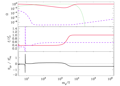
Figure 5: Same as Fig. 2 for the following parameters: $B_{\chi}=0$, $\Gamma_{\sigma}=10^{-6}\Gamma_{\chi\chi|\rm f}$ and $\Omega_{\sigma}^{\rm(i)}=10^{-1}$ corresponding to $\Omega_{\sigma}^{<_{\rm d}}=0.66$.

Finally, Fig. 5 provides an example of the case in which the decay of curvaton to dark matter is forbidden, i.e. $B_{\chi}=0$. Since $\Omega_{\sigma}^{<_{\rm d}}\sim 1$, all of radiation is produced during the decay. However, dark matter nevertheless inherits part of the curvaton perturbation through the influence of this latter on the freeze-out, as is apparent at times $x\simeq 30-10^{3}$ in Fig. 5. Therefore the final $S_{\chi\gamma}$ isocurvature perturbation is not maximal, but of the order of 70%, as measured relatively to the initial $S_{\sigma\gamma}$.

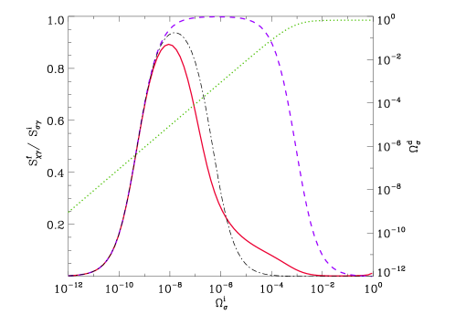
Figure 6: Final isocurvature perturbation $S_{\chi\gamma}$ expressed relatively to the initial $S_{\sigma\gamma}$ isocurvature perturbation (left $y-$axis), as a function of $\Omega_{\sigma}^{\rm(i)}$: numerical calculation (solid line), the analytical approximation given by Eq. (35) (dashed line) and a refined approximation taking into account the late time annihilation due to the curvaton decay (dotted-dashed line). The dotted line indicates the corresponding value of $\Omega_{\sigma}^{<_{\rm d}}$ (right $y-$axis) for convenience. The parameters are chosen to be: $\Gamma_{\sigma}/\Gamma_{\chi\chi|\rm f}=10^{-6}$ and $B_{\chi}=10^{-1}$.

IV.2 Final isocurvature perturbation

In a second series of figures, we explore the dependence of $S_{\chi\gamma}^{\rm(f)}/S_{\sigma\gamma}^{\rm(i)}$ on the initial abundance of the curvaton (or, equivalently, its abundance at the time of decay, $\Omega_{\sigma}^{<_{\rm d}}$) for different values of the branching ratio $B_{\chi}$ of curvaton to dark matter, and compare the numerical results to the analytical formulae.

In Fig. 6, the branching ratio is chosen as $B_{\chi}=0.1$. Let us describe this plot in more details. For very small values of $\Omega_{\sigma}^{({\rm i})}$, there is no isocurvature perturbation (as expected). This is also the case for large values of $\Omega_{\sigma}^{({\rm i})}$, i.e. when dark matter and radiation mostly originate in curvaton decay and, hence, have a common origin. Moreover, from our previous discussion of the analytical calculations, one expects that $S_{\chi\gamma}^{\rm(f)}$ will be maximal as long as $B_{\chi}\Omega_{\sigma}^{>_{\rm f}}>\Omega_{\chi}^{>_{\rm f}}$ but $(1-B_{\chi})\Omega_{\sigma}^{<_{\rm d}}\ll\Omega_{\gamma}^{<_{\rm d}}\sim 1$; this region corresponds to the peak plateau of the dashed line in Fig. 6. Indeed, combining Eqs. (36), the condition $B_{\chi}\Omega_{\sigma}^{>_{\rm f}}\gg\Omega_{\chi}^{>_{\rm f}}$ reads:

$$B_{\chi}\Omega_{\sigma}^{\rm(i)}\gg 5\times 10^{-3}x_{\rm f}^{1/2}{\rm e}^{-x_{\rm f}}\ ,$$ (37)

with $x_{\rm f}^{1/2}\exp(-x_{\rm f})\simeq 0.92\times 10^{-8}$ for $x_{\rm f}=20$ while the condition $(1-B_{\chi})\Omega_{\sigma}^{<_{\rm d}}\ll 1$ can be written as:

$$(1-B_{\chi})\Omega_{\sigma}^{\rm(i)}\left(\frac{\Gamma_{\sigma}}{\Gamma_{\chi\chi|{\rm f}}}\right)^{-1/2}\ll 3x_{\rm f}^{-1}\ ,$$ (38)

since one assumes radiation domination all throughout and $x_{\rm i}=3$. Recall that the ratio $\Gamma_{\sigma}/\Gamma_{\chi\chi|{\rm f}}$ represents the ratio of the Hubble factors at curvaton decay and at freeze-out.

As an example, consider the case depicted in Fig. 6: $x_{\rm f}=20$, $\Gamma_{\sigma}/\Gamma_{\chi\chi|\rm f}=10^{-6}$ and $B_{\chi}=10^{-1}$. Condition (37) shows that significant isocurvature perturbation can be produced when $\Omega_{\sigma}^{\rm(i)}\gtrsim 4.6\times 10^{-10}$, which agrees well with the results shown in Fig. 6. Condition (38) further limits this region to $\Omega_{\sigma}^{\rm(i)}\lesssim 1.7\times 10^{-4}$, which, again, agrees with the limit of the dashed line (analytical calculation).

Despite the above considerations, one notices in Fig. 6 that, when $S_{\chi\gamma}^{\rm(f)}/S_{\sigma\gamma}^{\rm(i)}$ is significant and $\Omega_{\sigma}^{\rm(i)}$ not too small, there is a mismatch between the analytical and numerical results by a factor of a few to an order of magnitude over most of the above parameter space. The reason of this discrepancy has been alluded to earlier; it lies in the neglect of the annihilation term in the post-freeze-out era. If a sufficient number of dark matter particles are produced during curvaton decay, this term may become significant, even at values $x\gg x_{\rm f}$, and regenerates some form of coupling between dark matter and radiation, leading to the partial or nearly complete erasure of the isocurvature perturbation. One can actually observe a typical example of the evolution of $S_{\chi\gamma}$ under the influence of regenerated dark matter annihilations in Fig. 2 at times $x\simeq 10^{3.6}\rightarrow 10^{4}$: the isocurvature perturbation decreases slightly to achieve its final value during this time interval; the impact of annihilations on $\Omega_{\chi}$ is not apparent in this figure but becomes clear if one plots $\Omega_{\chi}/a\propto a^{3}n_{\chi}$. Note that dark matter annihilations at around the time of big-bang nucleosynthesis may have interesting phenomenological consequences and distinct astrophysical signatures, see notably Ref. [17].

One can assess the range of parameters in which the annihilation term becomes significant, hence the analytical calculation inaccurate, as follows. If curvaton decay is instantaneous and all of dark matter originates in this decay (so as to produce a substantial $S_{\chi\gamma}$), one has: $\Omega_{\chi}^{>_{\rm d}}\,\simeq\,B_{\chi}\Omega_{\sigma}^{<_{\rm d}}$. After curvaton decay, one must compare the influence of the terms scaling with $\langle\sigma_{\chi\chi}v\rangle$ in Eq. (12) with the terms due to expansion. Since $\Delta_{\chi}$ and $\Phi$ are of the same order of magnitude, it suffices to compare the prefactors; furthermore, $\Omega_{\chi,{\rm eq}}\ll\Omega_{\chi}$ when $x\gg x_{\rm f}$, so that, finally, the analytical calculation should be valid provided:

$$\frac{3H\langle\sigma_{\chi\chi}v\rangle m_{\mathrm{Pl}}^{2}}{8\pi m_{\chi}}\Omega_{\chi}\ll 1\ .$$ (39)

Of course, it is understood that all terms in this equation should be evaluated immediately after curvaton decay. Since $\Omega_{\chi}=n_{\chi}m_{\chi}/\rho$, using the Friedmann equation one can rewrite the above constraint in the more intuitive way:

$$\Upsilon\,\equiv\,\frac{\Gamma_{\chi\chi}^{>_{\rm d}}}{H^{>_{\rm d}}}\,\ll\,1\ ,$$ (40)

which indeed expresses the fact that dark matter annihilations do not occur since the annihilation rate remains smaller than the Hubble rate. Note also that, in this sudden decay approximation, annihilations cannot occur in the interval separating freeze-out from curvaton decay.

Alternatively, one can discuss the case in which curvaton decay is not instantaneous, assuming here as well that $\Omega_{\chi}^{>_{\rm d}}\,\simeq\,B_{\chi}\Omega_{\sigma}^{<_{\rm d}}$. One must now compare the influence of the terms scaling with $\langle\sigma_{\chi\chi}v\rangle$ in Eq. (12) with the term due to curvaton decay, which leads to the following condition:

$$\frac{3H\langle\sigma_{\chi\chi}v\rangle m_{\mathrm{Pl}}^{2}}{8\pi m_{\chi}}\Omega_{\chi}^{2}\ll B_{\chi}\frac{\Gamma_{\sigma}}{H}\Omega_{\sigma}\ ,$$ (41)

at all times before curvaton decay. By considering the time evolution of the various terms, one can convince oneself that the l.h.s. increases faster with $x$ than the r.h.s. Let us discuss this last point in greater detail. The r.h.s. scales as $\propto x^{3}$ since $\Omega_{\sigma}\propto x$ and $H\propto x^{-2}$ in a radiation dominated phase. After freeze-out, but before curvaton decay, one might think that, in Eq. (7), only the term $\Omega_{\chi}\Omega_{\gamma}$ matters. In this case, $\Omega_{\chi}\propto x$ and the l.h.s. is constant, i.e. does not increase faster than the r.h.s. However, the influence of curvaton decay is felt before the time $H=\Gamma_{\sigma}$ so that the term proportional to $\Omega_{\sigma}$ in Eq. (7) cannot always be ignored. When this term dominates, $\Omega_{\chi}\propto x^{4}$ hence the l.h.s. indeed increases faster than the r.h.s. This scaling will last as long as the annihilation term remains negligible. When this latter becomes important, the evolution becomes such that the annihilation term and the term proportional to $\Omega_{\sigma}$ balance each other, thus scaling in the same way, which leads to $\Omega_{\chi}\propto x^{5/2}$ after the period where $\Omega_{\chi}\propto x^{4}$ and until $H=\Gamma_{\sigma}$. These considerations justify the fact that the l.h.s. increases faster than the r.h.s.; hence it suffices to evaluate the inequality (41) at the time of curvaton decay: if it is then satisfied, it will have always been verified prior to decay. After decay, of course, curvaton decay does not source anymore the evolution of $\Omega_{\chi}$ and all perturbations stay constant, as seen in previous figures. Since the time of curvaton decay is set by $H\sim\Gamma_{\sigma}$, and $\Omega_{\chi}^{>_{\rm d}}\sim B_{\chi}\Omega_{\sigma}^{<_{\rm d}}$, the previous condition of validity of the analytical calculation can be simplified down to the same condition (40) than obtained in the sudden decay approximation. In terms of our parameters, this reads:

$$B_{\chi}\Omega_{\sigma}^{\rm(i)}\left(\frac{\Gamma_{\sigma}}{\Gamma_{\chi\chi|{\rm f}}}\right)^{1/2}\,\ll\,5.0\times 10^{-3}x_{\rm f}^{1/2}{\rm e}^{-x_{\rm f}}\ .$$ (43)

Hence, the r.h.s. becomes $1.0\times 10^{-11}$ for $x_{\rm f}=20$. For the example considered above, namely $\Gamma_{\sigma}/\Gamma_{\chi\chi|\rm f}=10^{-6}$ and $B_{\chi}=10^{-1}$, condition (43) shows that the isocurvature perturbation remains maximal as long as: $\Omega_{\sigma}^{\rm(i)}\lesssim 4.6\times 10^{-7}$, in good agreement with Fig. 6.

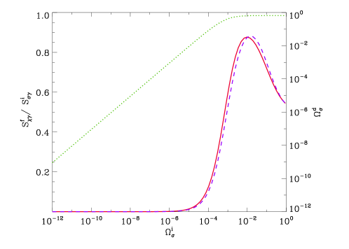
Figure 7: Same as Fig. 6, but for $B_{\chi}=0$.

In order to model the effect of regenerated annihilations on the perturbations, one can proceed as follows. One can study the evolution of $\zeta_{\chi}$ and $\zeta_{\gamma}$ after curvaton decay, assumed to be instantaneous for simplicity. In this case, one can safely neglect the first term in Eq. (7) since it is proportional to $\Omega_{\sigma}$ and the last term proportional to $\Omega_{\chi,{\rm eq}}$ as before. If one further considers that radiation dominates (hence $\Omega_{\gamma}\simeq 1$), then Eq. (7) can integrated exactly and the solution reads

$$\Omega_{\chi}=\Omega_{\chi}^{>_{\rm d}}\frac{\left(x/x_{\rm d}\right)^{2}}{\Upsilon\left[\left(x/x_{\rm d}\right)-1\right]+\left(x/x_{\rm d}\right)}\,,$$ (44)

where $x_{\rm d}$ is the time of curvaton decay. Then, making the same assumptions as before in Eq. (17) and considering that $\Phi$ remains constant (which is well-verified numerically), one obtains

$$\Delta_{\chi}+\Phi=\left[\Delta_{\chi}^{>_{\rm d}}+\Phi^{{}_{\rm d}}\right]\frac{\left(x/x_{\rm d}\right)}{\Upsilon\left[\left(x/x_{\rm d}\right)-1\right]+\left(x/x_{\rm d}\right)}\,.$$ (45)

Using this solution and the fact that $\Delta_{\gamma}\simeq-2\Phi$ is constant, one can estimate the amplitude of the isocurvature perturbations well after the curvaton decay. Straightforward manipulations leads to

$$S_{\chi\gamma}^{\rm(f)}=\frac{1}{1+\Upsilon}S_{\chi\gamma}^{>_{\rm d}}+\frac{\Upsilon}{2\left(\Upsilon+1\right)}\Phi^{>_{\rm d}}\,.$$ (46)

This result indicates that the final isocurvature perturbation is suppressed by a factor $(1+\Upsilon)$ which becomes all the more important as annihilations are effective at curvaton decay. This is reminiscent of the Weinberg theorem of the approach to adiabaticity (i.e. the erasure of isocurvature perturbations) of interacting fluids (here, dark matter and radiation through annihilations), although the physical conditions are here quite different, see Appendix C.

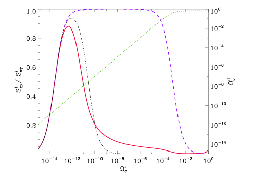
Figure 8: Same as Fig. 6, but for $x_{\rm f}=30$.

From our numerical experiments for different values of the parameters, we find that this reduction factor reproduces well the numerical results. For instance, in Fig. 6, the suppression factor manifests itself by a reduction of $S_{\chi\gamma}^{\rm(f)}$ for $\Omega_{\sigma}^{\rm(i)}\mathrel{\hbox to0.0pt{\lower 3.0pt\hbox{$\mathchar 536\relax$}\hss}\raise 2.0pt\hbox{$\mathchar 318\relax$}}4.6\times 10^{-7}$, as indicated by the dotted-dashed curve which agrees well with the numerical calculations. However, the presence or functional form of the second term in the r.h.s. of Eq. (46) is not confirmed by numerical experiments in which $S_{\chi\gamma}^{>_{\rm d}}=0$; one finds, in particular, $S_{\chi\gamma}^{\rm(f)}\simeq 0$ in this case. This error is attributable to the assumption of instantaneous curvaton decay, as we have checked numerically. Nevertheless, even if this term is included in the formula (as done in the comparison to the numerical results in Figs. 6,8), the agreement remains quite reasonable.

Let us now describe Fig. 7. It shows an altogether different scenario, in which the branching ratio $B_{\chi}=0$, i.e. the curvaton decays only into radiation. In this case, significant isocurvature is produced when $\Omega_{\sigma}^{<_{\rm d}}\sim 1$, as discussed before. In this case, the analytical calculation always agrees quite well with the numerical results. The isocurvature perturbation tends to decrease as $\Omega_{\sigma}^{\rm(i)}$ exceeds $\simeq 10^{-2}$ because the curvaton energy density at the time of freeze-out [$\Omega_{\sigma}^{>_{\rm f}}\sim 6\Omega_{\sigma}^{\rm(i)}$ for $x_{\rm f}=20$] then becomes significant. As a consequence, the dark matter curvature perturbation is affected by that of the curvaton, hence the final dark matter - radiation isocurvature is reduced.

Let us turn to Fig. 8. It shows an example similar to Fig. 6 for a different value of $x_{\rm f}$, here $x_{\rm f}=30$. The phenomenology is similar to that discussed for Fig. 6; the main difference lies in the much lower values of $\Omega_{\sigma}^{\rm(i)}$ where the isocurvature perturbation is maximal. Since $x_{\rm f}$ is larger than in Fig. 6, the post-freeze-out dark matter abundance is (much) smaller, hence a lesser degree of contamination by curvaton decay is sufficient to produce a substantial isocurvature perturbation. One can use the formulae (37), (38) and (43) to give a detailed account of Fig. 8.

Finally, in a third series of figures, we show the same value $S_{\chi\gamma}^{\rm(f)}/S_{\sigma\gamma}^{\rm(i)}$ in the plane of the branching ratio $B_{\chi}$ and initial curvaton abundance $\Omega_{\sigma}^{\rm(i)}$. The location of the peak of the isocurvature abundance, as shown in Fig. 9, follows the trend described above. Indeed, one sees two main regions where the relative isocurvature perturbation is of order unity, one at large branching ratio and small curvaton abundance, which corresponds to the case in which the curvaton decay produces a substantial amount of dark matter but negligible radiation, and the other at small branching ratio but large curvaton abundance, corresponding to the opposite limit.

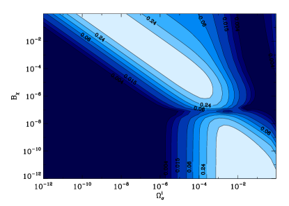
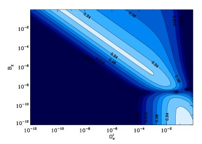
Figure 9: Contour plot of $S_{\chi\gamma}^{\rm(f)}/S_{\sigma\gamma}^{\rm(i)}$ in the plane $\Omega_{\sigma}^{\rm(i)}$, $B_{\chi}$, for $x_{\rm f}=20$. Each contour represents a decrement by a factor 2. In the left panel, $\Gamma_{\sigma}/\Gamma_{\chi\chi|\rm f}=10^{-6}$; in the right panel, $\Gamma_{\sigma}/\Gamma_{\chi\chi|\rm f}=10^{-3}$.

The right panel of Fig. 9 shows a plot similar to that in the left panel, albeit for a much larger value $\Gamma_{\sigma}/\Gamma_{\chi\chi|\rm f}=10^{-3}$, meaning that curvaton decay occurs shortly after dark matter freeze-out (at $x_{\rm d}\sim 10^{2}$). Consequently, secondary dark matter annihilations due to curvaton decay are more effective and restrain the part of parameter space where the isocurvature perturbation is maximal. The lower region is also pushed to larger values of $\Omega_{\sigma}^{\rm(i)}$ since, at given $\Omega_{\sigma}^{\rm(i)}$, an earlier curvaton decay means a smaller value of $\Omega_{\sigma}^{<_{\rm d}}$.

V Conclusion

In this article, we have constructed a comprehensive model of curvaton cosmology including radiation, WIMP dark matter (neutralinos) and a massive curvaton field modeled as a perfect fluid with a dust-like equation of state. We have computed the evolution of cosmological fluctuations through dark matter freeze-out and curvaton decay by approximate analytical methods as well as with a fully exact numerical treatment. As a result, we determine the final curvature and isocurvature perturbations and define the parameters that control their amplitude.

First of all, we have confirmed some results that are intuitively clear. There is obviously no production of isocurvature perturbations if the curvaton contribution is completely negligible or if, on the contrary, radiation and dark matter both come entirely from curvaton decay. Another case where the final $S_{\chi\gamma}$ vanishes is when the curvaton decays before dark matter freeze-out: because dark matter and radiation then share thermal equilibrium after curvaton decay, the isocurvature mode is erased in agreement with the theorem of Weinberg on the approach to adiabaticity for interacting fluids [11].

Our main finding is that a substantial radiation-dark matter isocurvature mode can be produced if either the dark matter or the radiation (but not both at the same time) mostly originates from curvaton decay. Quantitatively, the first situation corresponds to $B_{\chi}\Omega_{\sigma}^{<_{\rm d}}\mathrel{\hbox to0.0pt{\lower 3.0pt\hbox{$\mathchar 536\relax$}\hss}\raise 2.0pt\hbox{$\mathchar 318\relax$}}\Omega_{\chi}^{<_{\rm d}}$ and $\left(1-B_{\chi}\right)\Omega_{\sigma}^{<_{\rm d}}\ll\Omega_{\gamma}^{<_{\rm d}}$ (we recall that $B_{\chi}$ denotes the branching ratio of curvaton decay into dark matter, and that the symbol $<_{\rm d}$ is intended to mean “immediately before curvaton decay”). Despite the fact that the curvaton is underdominant at its decay, its influence on dark matter is important because the dark matter energy density is itself even smaller. The second regime corresponds to $B_{\chi}\sim 0$ and $\Omega_{\sigma}^{<_{\rm d}}\mathrel{\hbox to0.0pt{\lower 3.0pt\hbox{$\mathchar 536\relax$}\hss}\raise 2.0pt\hbox{$\mathchar 318\relax$}}\Omega_{\gamma}^{<_{\rm d}}$. In this case, at decay, the curvaton perturbations are mainly transferred to radiation. The curvaton perturbations also modifies the freeze-out at the perturbative level, thereby contaminating the dark matter fluctuations. Nevertheless, a significant radiation-dark matter isocurvature mode (as measured relatively to the curvature perturbation) is also produced in this limit.

Another important effect that we have observed and modeled is that regenerated dark matter at curvaton decay may annihilate, leading to a partial (or even complete) erasure of any previously existing $S_{\chi\gamma}$ isocurvature perturbation, even if the curvaton energy density at that time is small, $\Omega_{\sigma}^{<_{\rm d}}\ll 1$. Assuming the curvaton decay to be instantaneous, we have provided a new analytical formula describing this phenomenon which reproduces fairly well our exact numerical estimates. These late time annihilations further restrict the region in the parameter space of the model (in particular the value of the initial curvaton energy density) where significant isocurvature perturbations can be produced.

Appendix A Perturbations to first order

In this first appendix, one briefly recalls how the gauge-invariant equations of motion of the (scalar) perturbations used in the main text, see Eqs. (12)–(15), can be obtained. The scalar part of the perturbed metric can be expressed as [18, 19]

$${\rm d}s^{2}=a^{2}(\eta)\left\{-(1+2\phi){\rm d}\eta^{2}+2\partial_{i}B{\rm d}x^{i}{\rm d}\eta+\left[\left(1-2\psi\right)\delta_{ij}+2\partial_{i}\partial_{j}E\right]{\rm d}x^{i}{\rm d}x^{j}\right\}\ ,$$ (47)

and depends on four unknown functions: $\phi$, $B$, $\psi$ and $E$. In the previous expression, $a(\eta)$ is the Friedmann-Lemaître-Robertson-Walker scale factor and $\eta$ denotes the conformal time. The most general (infinitesimal) change of coordinates (or “gauge-transformation”) that can be constructed with scalar functions (given here by $\xi^{0}$ and $\xi$) is given by

$$\eta\rightarrow\bar{\eta}=\eta+\xi^{0}(\eta,x^{k}),\quad x^{i}\rightarrow\bar{x}^{i}=x^{i}+\delta^{ij}\partial_{j}\xi(\eta,x^{k})\,.$$ (48)

Calculating the Lie derivative along the four vector defined above, we find that the four scalar functions used to construct the scalar perturbed metric transform according to

$$\bar{\phi}=\phi+\xi^{0^{\prime}}+\frac{a^{\prime}}{a}\xi^{0},\quad\bar{B}=B-\xi^{0}+\xi^{\prime},\quad\bar{\psi}=\psi-\frac{a^{\prime}}{a}\xi^{0},\quad\bar{E}=E+\xi\,,$$ (49)

where a prime denotes derivative with respect to conformal time. As a consequence, the following combinations, known as the Bardeen potentials

$$\Phi\equiv\phi+\frac{1}{a}\left[a\left(B-E^{\prime}\right)\right]^{\prime},\quad\Psi\equiv\psi-\frac{a^{\prime}}{a}\left(B-E^{\prime}\right)\,,$$ (50)

are gauge invariant, that is to say, $\bar{\Phi}=\Phi$ and $\bar{\Psi}=\Psi$. In particular, $\Phi$ can be viewed as the relativistic generalization of the Newtonian potential.

One must also construct gauge-invariant combinations for the scalar quantities appearing in the perturbed stress-energy tensor. The rule of transformation of the stress-energy tensor is that of any two-rank tensor and has already been given above. In the following, we consider the case where several fluids are present and we denote each species by the index “$(\alpha)$”. Then, straightforward manipulations lead to:

$$\bar{\delta\rho_{(\alpha)}}=\delta\rho_{(\alpha)}+\rho_{(\alpha)}^{\prime}\xi^{0}\,\quad\bar{v_{(\alpha)}}=v_{(\alpha)}-\xi^{\prime}\,\quad\bar{\delta p_{(\alpha)}}=\delta p_{(\alpha)}+p_{(\alpha)}^{\prime}\xi^{0}\,,$$ (51)

where $\rho_{(\alpha)}$, $p_{(\alpha)}$ and $v_{(\alpha)}$ are respectively the background energy density, pressure and velocity of the fluid “$(\alpha)$”. For the quantities describing the matter, these expressions play the same role as Eqs. (49) for the metric perturbations. From these expressions, one can easily construct gauge-invariant density contrast, pressure and velocity perturbations, namely

$$\Delta\rho_{(\alpha)}\,=\,\delta\rho_{(\alpha)}+\rho_{(\alpha)}^{\prime}\left(B-E^{\prime}\right)\,,\qquad\Delta p_{(\alpha)}\,=\,\delta p_{(\alpha)}+p_{(\alpha)}^{\prime}(B-E^{\prime}),\qquad V_{(\alpha)}=v_{(\alpha)}+E^{\prime}\,.$$ (52)

The equations of motion for these quantities can be obtained from the perturbed Einstein equations or from the time and space components of the conservation equation, the two methods being equivalent thanks to the Bianchi identities.

In the presence of multiple interacting fluids, which is the case of interest in the present article, one must include the various energy transfer rates between the different fluids. One may express these transfers in the form:

$$\nabla_{\mu}T^{\mu\nu}_{(\alpha)}=Q^{\nu}_{(\alpha)}+Y^{\nu}_{(\alpha)}\,,$$ (53)

where the vector $Q^{\nu}_{(\alpha)}$ represents the case of a decay and must be linear in energy density while $Y^{\nu}_{(\alpha)}$ describes the case of annihilations and must thus be quadratic in energy density. This suggests the following covariant writing for the transfer related to decay

$$Q^{\mu}_{(\alpha)}=\Gamma_{\sigma(\alpha)}T^{\mu\nu}_{\sigma}u_{\nu}=-\Gamma_{\sigma(\alpha)}\rho_{\sigma}u^{\mu}\,,$$ (54)

$\Gamma_{\sigma(\alpha)}$ being the decay rate of species $\sigma$ to species $(\alpha)$; the above equations holds for a source, not a loss term. In addition, the previous expression is valid if the stress-energy tensor is that of a perfect fluid. As far as annihilation terms are concerned, the analog $Y^{\mu}_{(\alpha)}$ of the transfer rate $Q^{\mu}_{(\alpha)}$ can be written as

$$Y^{\mu}_{(\alpha)}=\frac{\left\langle\sigma_{\chi\chi}v\right\rangle_{(\alpha)}}{m_{(\alpha)}}\left[T^{\mu}_{(\alpha)}{}_{\lambda}T^{\lambda\beta}_{(\alpha)}-T^{\mu}_{(\alpha),{\rm eq}}{}_{\lambda}T^{\lambda\beta}_{(\alpha),{\rm eq}}\right]u_{\beta}=\frac{\left\langle\sigma_{\chi\chi}v\right\rangle_{(\alpha)}}{m_{(\alpha)}}\left[\rho^{2}_{(\alpha)}-\rho_{(\alpha),{\rm eq}}^{2}\right]u^{\mu}\,.$$ (55)

In this expression $T^{\mu\nu}_{(\alpha),{\rm eq}}$ is the stress-energy tensor of the fluid “$(\alpha)$” in thermal equilibrium. In particular, the corresponding energy density is given by Eq. (3). As before, the last equation has been obtained postulating a perfect fluid. Of course the total stress-energy tensor is conserved and, therefore, one has:

$$\nabla_{\mu}\left[\sum_{\alpha}T_{(\alpha)}^{\mu\nu}\right]=\sum_{\alpha}\left[Y_{(\alpha)}^{\nu}+Q_{(\alpha)}^{\nu}\right]=0\,.$$ (56)

One advantage of the previous covariant formalism is that the transformation properties of the vectors $Q_{\mu}$ and $Y_{\mu}$ can now be evaluated quite easily. Using Eqs. (54) and (55), one finds:

$$\delta Q^{\mu}_{(\alpha)} = \Gamma_{\sigma(\alpha)}\left[\delta T^{\mu\nu}_{\sigma}u_{\nu}+T^{\mu\nu}_{\sigma}\delta u_{\nu}\right]\,,$$ (57)

$$\delta Y^{\mu}_{(\alpha)} = \frac{\langle\sigma_{\chi\chi}v\rangle_{(\alpha)}}{m_{(\alpha)}}\Biggl{[}\delta T^{\mu}_{(\alpha)}{}_{\lambda}T_{(\alpha)}^{\lambda\beta}u_{\beta}+T^{\mu}_{(\alpha)}{}_{\lambda}\delta T_{(\alpha)}^{\lambda\beta}u_{\beta}+T^{\mu}_{(\alpha)}{}_{\lambda}T_{(\alpha)}^{\lambda\beta}\delta u_{\beta}-\delta T^{\mu}_{(\alpha),{\rm eq}}{}_{\lambda}T_{(\alpha),{\rm eq}}^{\lambda\beta}u_{\beta}-T^{\mu}_{(\alpha),{\rm eq}}{}_{\lambda}\delta T_{(\alpha),{\rm eq}}^{\lambda\beta}u_{\beta}$$ (58)

$$-T^{\mu}_{(\alpha),{\rm eq}}{}_{\lambda}T_{(\alpha),{\rm eq}}^{\lambda\beta}\delta u_{\beta}\Biggr{]}\,.$$

Working out the above expressions for the time component, this gives

$$\delta Q_{(\alpha)0}=a\Gamma_{\sigma(\alpha)}\left[\delta\rho_{\sigma}+\rho_{\sigma}\phi\right]\,,\qquad\delta Y_{(\alpha)0}=\frac{\langle\sigma_{\chi\chi}v\rangle_{(\alpha)}}{m_{(\alpha)}}\left\{-2a\left[\rho_{(\alpha)}\delta\rho_{(\alpha)}-\rho_{(\alpha),{\rm eq}}\delta\rho_{(\alpha),{\rm eq}}\right]-a\left[\rho^{2}_{(\alpha)}-\rho^{2}_{(\alpha),{\rm eq}}\right]\phi\right\}\,,$$ (59)

where we have used that $\delta u^{0}=-\phi/a$. Then, the time component of the conservation equation leads to the following gauge-invariant equation, for instance for the dark matter component:

$$\Delta\rho_{\chi}^{\prime}+3{\cal H}\left(\Delta\rho_{\chi}+\Delta p_{\chi}\right)-3\left(\rho_{\chi}+p_{\chi}\right)\Phi^{\prime}+\left(\rho_{\chi}+p_{\chi}\right)\partial_{k}\partial^{k}V_{\chi}=a\Gamma_{\chi}\left(\Delta\rho_{\chi}+\rho_{\chi}\Phi\right)$$

$$-\frac{\langle\sigma_{\chi\chi}v\rangle}{m_{\chi}}a\left[2\rho_{\chi}\Delta\rho_{\chi}-2\rho_{\chi,{\rm eq}}\Delta\rho_{\chi,{\rm eq}}+\left(\rho_{\chi}^{2}-\rho^{2}_{\chi,{\rm eq}}\right)\Phi\right]\,.$$ (60)

On large scales the gradient of the velocity term can be neglected. Then, the above equation exactly reduces to Eq. (12) used in the main body of the text. Other equations (13) and (14) are obtained along the same lines.

Appendix B Junction conditions

The junction conditions allow us to derive how the “conserved” quantities cross freeze-out. Assuming that the spatial transition hypersurface $\Sigma$ is defined by the condition that some function $q=q_{0}+\delta q$ remains constant, its normal $n^{\mu}$ is given by $n_{\mu}=\partial_{\mu}q$ and, then, two conditions must be fulfilled[20, 21] so that the two space-time manifolds along $\Sigma$ can be joined without a surface layer: the induced spatial metric $\perp_{ij}$ obtained from $\perp_{\mu\nu}\equiv g_{\mu\nu}+n_{\mu}n_{\nu}$ and the extrinsic curvature (or second fundamental form) $K_{ij}$ should be continuous on $\Sigma$, i.e.

$$\left[\perp_{ij}\right]_{\pm}=0\,,\quad\left[K_{ij}\right]_{\pm}=0\,.$$ (61)

The extrinsic curvature is defined as:

$$K_{\mu\nu}=-\frac{1}{2}{\cal L}_{n}\perp_{\mu\nu}=-\frac{1}{2}\left(n^{\rho}\nabla_{\rho}\perp_{\mu\nu}+\perp_{\rho\nu}\nabla_{\mu}n^{\rho}+\perp_{\rho\mu}\nabla_{\nu}n^{\rho}\right)\,,$$ (62)

where ${\cal L}_{n}$ denotes the Lie derivative with respect to the normal $n^{\mu}$. In order to compute $K_{ij}$ the system of coordinates (i.e. the gauge) and the vector $n^{\mu}$ (i.e. the surface of transition) have to be specified. Different choices for $n^{\mu}$ lead to inequivalent junction conditions. The previous equations are the general rules that must applied in order to find the matching conditions. Expressing the condition $\left[\delta\perp_{ij}\right]_{\pm}=0$ for diagonal and off-diagonal terms leads to:

$$\left[\psi\left(\eta_{{}_{\Sigma}}\right)\right]_{\pm}=\left[\psi+{\cal H}\frac{\delta q}{q_{0}^{\prime}}\right]_{\pm}\left(\eta_{0}\right)=0\,,\qquad\left[E\left(\eta_{{}_{\Sigma}}\right)\right]_{\pm}=\left[E\left(\eta_{0}\right)\right]_{\pm}=0\,,$$ (63)

where we have used that $\eta_{{}_{\Sigma}}=\eta_{0}+\delta\eta$. Repeating the same calculation for the second fundamental form gives two other (gauge-invariant) junction conditions, namely

$$\left[\psi^{\prime}+{\cal H}\phi+\left({\cal H}^{\prime}-{\cal H}^{2}\right)\frac{\delta q}{q_{0}^{\prime}}\right]_{\pm}\left(\eta_{0}\right)=0\,,\qquad\left[B-E^{\prime}+\frac{\delta q}{q_{0}^{\prime}}\right]_{\pm}\left(\eta_{0}\right)=0\,.$$ (64)

The equations (63) and (64) represent the complete set of matching conditions for density perturbations. Let us now derive the consequences of these equations. Since $\left[\psi\right]_{\pm}=-{\cal H}\left[\delta q/q_{0}^{\prime}\right]_{\pm}$, $\left[B-E^{\prime}\right]_{\pm}=-\left[\delta q/q_{0}^{\prime}\right]_{\pm}$ and $\left[\Psi\right]_{\pm}=\left[\Phi\right]_{\pm}=\left[\psi\right]_{\pm}-{\cal H}\left[B-E^{\prime}\right]_{\pm}$ (the first equation of this last relation simply comes from the fact that we assume $\Phi=\Psi$), we deduce that

$$\left[\Phi\right]_{\pm}=0\,.$$ (65)

This condition does not depend on which quantity $q$ we choose and is therefore hypersurface independent. On the other hand, to obtain the other condition, we must specify this quantity. For the particular case of dark matter annihilation freeze-out, the transition is determined by the quantity

$$q_{0}=\frac{\Gamma}{H}\,.$$ (66)

Before freeze out one has $\Gamma/H\propto T^{\alpha}/\rho^{1/2}$ and this leads to

$$\left(-\psi-{\cal H}\frac{\delta q}{q_{0}^{\prime}}\right|_{<_{\rm f}}=\zeta_{\gamma}^{<_{\rm f}}+\frac{3\Omega_{\sigma}\left(\zeta_{\sigma}^{<_{\rm f}}-\zeta_{\gamma}^{<_{\rm f}}\right)}{\left[2\left(2-\alpha\right)-\Omega_{\sigma}\right]}+{\cal O}\left(\Omega_{\chi}\right)\,.$$ (67)

After freeze-out, one has $\Gamma n_{\chi}\langle\sigma_{\chi\chi}v\rangle\propto\rho_{\chi}$. This leads to

$$\left(-\psi-{\cal H}\frac{\delta q}{q_{0}^{\prime}}\right|_{>_{\rm f}}=\zeta_{\chi}^{>_{\rm f}}+\frac{2}{2+\Omega_{\sigma}}\left[\left(2-\frac{1}{2}\Omega_{\sigma}\right)\zeta_{\chi}^{>_{\rm f}}-\frac{3}{2}\Omega_{\sigma}\zeta_{\sigma}^{>_{\rm f}}-2\left(1-\Omega_{\sigma}\right)\zeta_{\gamma}^{>_{\rm f}}\right]\,.$$ (68)

Equating these two expressions and using the fact that $\zeta_{\gamma}^{<_{\rm f}}=\zeta_{\gamma}^{>_{\rm f}}$ and $\zeta_{\sigma}^{<_{\rm f}}=\zeta_{\sigma}^{>_{\rm f}}$, one arrives at

$$\zeta_{\chi}^{>_{\rm f}}=\zeta_{\gamma}^{<_{\rm f}}+\frac{\left(\alpha-3\right)\Omega_{\sigma|{\rm f}}}{2\left(\alpha-2\right)+\Omega_{\sigma|{\rm f}}}\left(\zeta_{\sigma}^{<_{\rm f}}-\zeta_{\gamma}^{<_{\rm f}}\right)\,,$$ (69)

where the background quantities are evaluated at the time of freeze-out and where we recall that $\alpha=m/T+3/2$ evaluated at the freeze-out. We have thus recovered, by means of the junction conditions, Eq. (22) used in the text and derived for the first time (although using different techniques) in Ref. [9].

Appendix C Approach to adiabaticity for interacting fluids

In this last appendix, we discuss the theorem proved by Weinberg [11], according to which any pre-existing isocurvature perturbation between two interacting fluids is rapidly erased at thermal equilibrium. In addition, we explicitly calculate the typical time scale of this phenomenon in the present context and compare the analytical prediction to numerical calculations.

The number density of dark matter particles evolves according to $n^{\prime}+3{\cal H}n=Y_{0}/m_{\chi}$, with $Y_{0}/m_{\chi}=-a\langle\sigma_{\chi\chi}v\rangle\left(n^{2}-n_{\rm eq}^{2}\right)$, in the absence of curvaton decays but accounting for $\chi-\chi$ annihilations. This equation cannot be solved explicitly but useful information can be obtained by linearizing it. For this purpose, one writes $n=n_{\rm eq}+\delta n$ where $\delta n\ll n_{\rm eq}$. Then, the equation obeyed by $\delta n$ reads, to first order in $\delta n/n_{\rm eq}$:

$$\frac{{\rm d}}{{\rm d}t}\left(a^{3}\delta n\right)+2\langle\sigma_{\chi\chi}v\rangle n_{\rm eq}a^{3}\delta n=-\frac{{\rm d}}{{\rm d}t}\left(a^{3}n_{\rm eq}\right)\,,$$ (70)

whose solution can be expressed as:

$$\delta n\,=\,\delta n(t_{\rm i})\left[\frac{a(t_{\rm i})}{a(t)}\right]^{3}\eta(t_{\rm i};\,t)-\frac{1}{a^{3}}\int_{t_{\rm i}}^{t}{\rm d}\theta\frac{\rm d}{{\rm d}\theta}\left(a^{3}n_{\rm eq}\right)\eta(\theta;\,t)\ ,$$ (71)

where we have defined the function:

$$\eta(t^{\prime};\,t)\,\equiv\,\exp\left(-2\int_{t^{\prime}}^{t}{\rm d}\tau\,\langle\sigma_{\chi\chi}v\rangle n_{\rm eq}\right)\ .$$ (72)

As long as $x<x_{\rm f}$, the integrand (annihilation rate) $\langle\sigma_{\chi\chi}v\rangle n_{\rm eq}$ is very large compared to an inverse Hubble time, hence the function $\eta(t^{\prime};\,t)$ collapses to zero on a very short timescale $\sim\left[\langle\sigma_{\chi\chi}v\rangle n_{\rm eq}\right]^{-1}$. One can thus Taylor expand the integral to first order and write:

$$\eta(t^{\prime};\,t)\,\simeq\,\exp\left[-(t-t^{\prime})\times 2\langle\sigma_{\chi\chi}v\rangle n_{\rm eq}\right]\,\approx\,\frac{1}{\langle\sigma_{\chi\chi}v\rangle n_{\rm eq}(t^{\prime})}\delta\left(t-t^{\prime}\right)\,$$ (73)

using the following representation of the Dirac function, $\delta_{\epsilon}(x)={\rm e}^{-|x|/\epsilon}/(2\epsilon)$.

The first term on the r.h.s. of Eq. (71) corresponds to the difference at $t_{\rm i}$ between $n_{\rm eq}(t_{\rm i})$ and the solution of the evolution equation for $n$. This term collapses on the above short timescale due to the presence of the function $\eta(t_{\rm i};t)$. This timescale can be written in a compact way in terms of the $e-$fold number $N$, using the change of variables ${\rm d}t\,=\,{\rm d}N/H$:

$$\eta(t_{\rm i};\,t)\,\simeq\,\exp\left(-\frac{N-N_{\rm i}}{\Delta N}\right)\ ,$$ (74)

with:

$$\Delta N\,=\,\frac{H(t_{\rm i})}{2\langle\sigma_{\chi\chi}v\rangle_{t_{\rm i}}n_{\rm eq}(t_{\rm i})}\,\simeq\,\frac{1}{2\sqrt{x_{\rm f}x_{\rm i}}}{\rm e}^{-x_{\rm f}+x_{\rm i}}\ .$$ (75)

For $x_{\rm i}=3$ and $x_{\rm f}=20$, the number of $e-$folds necessary to erase any initial departure from the solution $n$ is: $\Delta N\simeq 2.67\times 10^{-9}$, very small indeed as compared to unity.

The second term on the r.h.s. of Eq. (71) represents the difference between $n$ and $n_{\rm eq}$. It will prove interesting for the discussion that follows to estimate the relative magnitude of this term. Assuming that $\delta n_{\rm i}=0$, one can re-express this term by changing variables ${\rm d}t={\rm d}\ln(x)/H$ in Eq. (71):

$$\delta n(x)\,=\,\int_{x_{\rm i}}^{x}{\rm d}x^{\prime}\left(\frac{x^{\prime}}{x}\right)^{3}\frac{x^{\prime}-3/2}{x^{\prime}}n_{\rm eq}(x^{\prime})\eta(x^{\prime};\,x)\,\simeq\,\frac{1}{2}\frac{x-3/2}{x}\left(\frac{x}{x_{\rm f}}\right)^{1/2}{\rm e}^{x-x_{\rm f}}n_{\rm eq}(x)\ ,$$ (76)

where we have approximated $\eta(x^{\prime};\,x)$ with the delta function in the last equality (the factor of $1/2$ comes from the fact that the Dirac function is peaked over the upper boundary of the integral). Hence $\delta n/n_{\rm eq}\sim{\cal O}\left(e^{x-x_{\rm f}}\right)\ll 1$ when $x<x_{\rm f}$.

Finally, by integrating by parts Eq. (71), one can write the global solution $n$ as:

$$n(t)\simeq\frac{n(t_{\rm i})}{a^{3}}\eta(t_{\rm i};\,t)+\frac{2}{a^{3}}\langle\sigma_{\chi\chi}v\rangle\int_{t_{\rm i}}^{t}a^{3}\left(\theta\right)n_{\rm eq}^{2}\left(\theta\right)\eta(\theta;\,t)\,{\rm d}\theta.$$ (77)

Here as well, the first term on the r.h.s. represents the initial value which collapses on a time scale $(2\langle\sigma_{\chi\chi}v\rangle n_{\rm eq})^{-1}$, while the second term can be shown to approximate $n_{\rm eq}$ to within the above $\delta n$.

Let us now turn the perturbed quantities. At the perturbed level the equation $\nabla_{\mu}n^{\mu}=0$ gives

$$\partial_{0}\delta n^{0}+\partial_{i}\delta n^{i}+4{\cal H}\delta n^{0}+\left(-3\psi^{\prime}+\partial_{i}\partial^{i}E^{\prime}+\phi^{\prime}\right)n^{0}=0\,.$$ (78)

The quadrivector $n_{\mu}$ can be written as $n_{\mu}=nu_{\mu}$ and, therefore, one has $\delta n_{0}=-a\left(\delta n+n\phi\right)$. Then, one can define the following gauge-invariant quantity

$$\Delta n=\delta n+n^{\prime}\left(B-E^{\prime}\right)\,,$$ (79)

and, on large scales, Eq. (78) reads

$$\Delta n^{\prime}+3{\cal H}\Delta n-3n\Psi^{\prime}=0\,.$$ (80)

This equation is nothing but Eq. (A) for a pressureless fluid since then $\rho=m_{\chi}n$. Again if one takes into account the interaction term, then the above equation becomes

$$\Delta n^{\prime}+3{\cal H}\Delta n-3n\Phi^{\prime}=\frac{\delta Y_{0}}{m_{\chi}}\,,$$ (81)

where (using again the relation $\rho=m_{\chi}n$) the explicit form of the annihilation term is given by Eq. (59), namely

$$\frac{\delta Y_{0}}{m_{\chi}}=-2a\langle\sigma_{\chi\chi}v\rangle\left(n\Delta n-n_{\rm eq}\Delta n_{\rm eq}\right)+\frac{Y_{0}}{m_{\chi}}\Phi\,,$$ (82)

where $\Delta n_{\rm eq}=n_{\rm eq}\Delta_{\rm eq}$, and $\Delta_{\rm eq}$ has been defined in Eq. (16). In particular, since $\Delta n_{\rm eq}$ is proportional to $\Delta\rho_{\gamma}$, its gauge-invariance is automatically guaranteed. In Ref. [9], the following quantity

$$\tilde{\zeta}_{\chi}\equiv-\Phi-{\cal H}\frac{\Delta n}{n^{\prime}}\,,$$ (83)

has been defined. This quantity is obviously gauge-invariant and, if $Q_{\mu}$ and $Y_{\mu}$ are not considered, is simply equal to $\zeta_{\chi}$. Then, let us consider the following combination

$$\frac{{\rm d}}{{\rm d}\eta}\left[-\frac{\Delta\rho_{\gamma}}{\rho_{\gamma}^{\prime}}\left(n^{\prime}+3{\cal H}n-\frac{Y_{0}}{m_{\chi}}\right)\right]+\Delta n^{\prime}+3{\cal H}\Delta n-3n\Phi^{\prime}-\frac{\delta Y_{0}}{m_{\chi}}=0\,.$$ (84)

Working out this expression, one obtains

$$\frac{{\rm d}}{{\rm d}\eta}\left(\Delta n-n^{\prime}\frac{\Delta\rho_{\gamma}}{\rho_{\gamma}^{\prime}}\right) = -3{\cal H}\left(\Delta n-n^{\prime}\frac{\Delta\rho_{\gamma}}{\rho_{\gamma}^{\prime}}\right)-2a\langle\sigma_{\chi\chi}v\rangle n\Delta n+2a\langle\sigma_{\chi\chi}v\rangle n_{\rm eq}\Delta n_{\rm eq}+\frac{Y_{0}}{m_{\chi}}\left[\Phi-\left(\frac{\Delta\rho_{\gamma}}{\rho_{\gamma}^{\prime}}\right)^{\prime}\right]$$ (85)

$$-\frac{Y_{0}^{\prime}}{m_{\chi}}\frac{\Delta\rho_{\gamma}}{\rho_{\gamma}^{\prime}}+3n\left[\Phi^{\prime}+{\cal H}^{\prime}\frac{\Delta\rho_{\gamma}}{\rho_{\gamma}^{\prime}}+{\cal H}\left(\frac{\Delta\rho_{\gamma}}{\rho_{\gamma}^{\prime}}\right)^{\prime}\right]\,.$$

This formula is exact. At this stage, one should make some approximations adapted to the situation at hands. Let us first assume that we are before freeze-out. According to the previous considerations, one can neglect $Y_{0}$ since its magnitude is of order $\delta n/n_{\rm eq}\ll 1$ ($x<x_{\rm f}$) as compared to the others. The previous equation then reduces to

$$\frac{{\rm d}}{{\rm d}\eta}\left(\Delta n-n^{\prime}\frac{\Delta\rho_{\gamma}}{\rho_{\gamma}^{\prime}}\right) = \left(-3{\cal H}-2a\langle\sigma_{\chi\chi}v\rangle n_{\rm eq}\right)\left(\Delta n-n^{\prime}\frac{\Delta\rho_{\gamma}}{\rho_{\gamma}^{\prime}}\right)+3n\left[\Phi^{\prime}+{\cal H}^{\prime}\frac{\Delta\rho_{\gamma}}{\rho_{\gamma}^{\prime}}+{\cal H}\left(\frac{\Delta\rho_{\gamma}}{\rho_{\gamma}^{\prime}}\right)^{\prime}\right]\,.$$ (86)

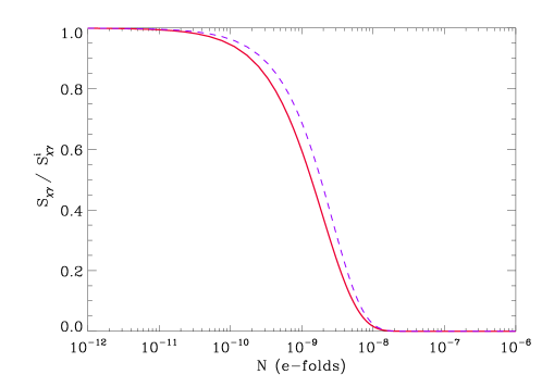
Figure 10: Evolution of the isocurvature perturbation $S_{\chi\gamma}$ [relative to the initial $S_{\chi\gamma}^{\rm(i)}$] during the first fractions of $e-$folds at $x\simeq 3$. The thick solid line shows the results of the numerical integration, and the dashed line that of the analytical calculation, given by Eq. (88).

Now, we further assume that freeze-out occurs in a radiation-dominated era. In this case, the quantity defined by $\zeta_{\gamma}\equiv-\Phi-{\cal H}\Delta\rho_{\gamma}/\rho_{\gamma}^{\prime}$ is conserved hence the term proportional to $3n$ vanishes. Therefore, using the fact that $n^{\prime}\simeq-{\cal H}n\left(x+3/2\right)$, the final equation reads

$$\frac{{\rm d}}{{\rm d}\eta}\left[\ln\left(\frac{\Delta n}{n}-\frac{n^{\prime}}{n}\frac{\Delta\rho_{\gamma}}{\rho_{\gamma}^{\prime}}\right)\right] = \left(x-\frac{3}{2}\right){\cal H}-2a\langle\sigma_{\chi\chi}v\rangle n_{\rm eq}\,.$$ (87)

However, before freeze-out, the first term in the right hand side of the above relation is much smaller than the second one and, hence, can be safely neglected. Finally, one arrives at

$$\tilde{\zeta}_{\chi}-\zeta_{\gamma}=\left(\tilde{\zeta}_{\chi}-\zeta_{\gamma}\right)_{\rm i}\frac{x_{\rm i}+3/2}{x+3/2}\eta(t_{\rm i};\,t)\,,$$ (88)

where the function $\eta(t_{\rm i};\,t)$ has already been computed in Eqs. (73) and (74).

This analytical result is compared to the numerical calculations in Fig. 10. Indeed, the agreement is excellent, and the numerical calculations confirm the erasure of any initial isocurvature perturbation $S_{\chi\gamma}$ on the $e-$fold scale $\Delta N\sim 3\times 10^{-9}$ computed in Eq. (75).

References

- [1] S. Mollerach, Phys. Lett. B 242, 158 (1990).
- [2] D. Lyth and D. Wands, Phys. Lett. B 524, 5 (2002), hep-ph/0110002.
- [3] A curvaton scenario was suggested in Ref. [4] as a way-out to overcome the difficulties of the pre-big-bang scenario in generating adiabatic perturbations; the corresponding calculations were provided in [5].
- [4] A. Buonanno, M. Lemoine and K. A. Olive, Phys. Rev. D 62, 083513 (2000), hep-th/0006054.
- [5] K. Enqvist and M. Sloth, Nucl. Phys. B 626, 395 (2002), hep-ph/0109214.
- [6] D. Lyth, C. Ungarelli and D. Wands, Phys. Rev. D 67, 023503 (2003), astro-ph/0208055.
- [7] T. Moroi and T. Takahashi, Phys. Lett B 522, 215 (2001), Erratum-ibid. B 539, 303 (2002), hep-ph/0110096; Phys. Rev. D 66, 063501 (2002), hep-ph/0206026.
- [8] A. Linde and V. Mukhanov, Phys. Rev. D 56, 535 (1997), astro-ph/9610219.
- [9] D. Lyth and D. Wands, Phys. Rev. D 68, 103516 (2003), astro-ph/0306500.
- [10] K. Enqvist, S. Kasuya and A. Mazumdar, Phys. Rev. Lett. 90, 091302 (2003), hep-ph/0211147; K. Dimopoulos, D. H. Lyth, A. Notari and A. Riotto, JHEP 0307, 053 (2003), hep-ph/0304050; S. Kasuya, M. Kawasaki, F. Takahashi, Phys. Lett. B 578, 259 (2004), hep-ph/0305134; R. Allahverdi, K. Enqvist, A. Jokinen and A. Mazumdar, JCAP 0610, 007 (2006), hep-ph/0603255.
- [11] S. Weinberg, Phys. Rev. D 70, 083522 (2004), astro-ph/0405397.
- [12] D. Langlois and F. Vernizzi, Phys. Rev. D 70, 063522 (2004), astro-ph/0403258.
- [13] S. Gupta, K. Malik and D. Wands, Phys. Rev. D 69, 063513 (2004), astro-ph/0311562.
- [14] K. Malik, D. Wands and C. Ungarelli, Phys. Rev. D 67, 063516 (2003), astro-ph/0211602.
- [15] F. Ferrer, S. Räsänen and J. Váliviita, JCAP 0410, 010 (2004), astro-ph/0407300.
- [16] E. Kolb and M. Turner, The Early Universe, Addison-Wesley (1990).
- [17] K. Jedamzik, Phys. Rev. D 70, 063524 (2004), astro-ph/0402344; Phys. Rev. D 70, 083510 (2004), astro-ph/0405583.
- [18] H. Kodama and M. Sasaki, Prog. Th. Phys. Supp 78, 1 (1984).
- [19] V. F. Mukhanov, H. A. Feldman and R. H. Brandenberger, Phys. Rep. 215, 203 (1992).
- [20] N. Deruelle and V. F. Mukhanov, Phys. Rev. D 52, 5549 (1995), gr-qc/9503050.
- [21] J. Martin and D. J. Schwarz, Phys. Rev. D 57, 3302 (1998), gr-qc/9704049.