Spectroscopy of Globular Clusters out to Large Radius in the Sombrero Galaxy

Abstract

We present new velocities for 62 globular clusters in M104 (NGC 4594, the Sombrero Galaxy), 56 from 2dF on the AAT and 6 from Hydra on WIYN. Combined with previous data, we have a total sample of 108 M104 globular cluster velocities, extending to 20′ radius ($\sim$ 60 kpc), along with BVR photometry for each of these. We use this wide-field dataset to study the globular cluster kinematics and dark matter content of M104 out to 10′ radius (30 kpc). We find no rotation in the globular cluster system. The edge-on nature of M104 makes it unlikely that there is strong rotation which is face-on and hence unobserved; thus, the absence of rotation over our large radial range appears to be an intrinsic feature of the globular cluster system in M104. We discuss ways to explain this low rotation, including the possibility that angular momentum has been transferred to even larger radii through galaxy mergers. The cluster velocity dispersion is $\sim$ 230 km/s within several arcmin of the galaxy center, and drops to $\sim$ 150 km/s at $\sim$ 10′ radius. We derive the mass profile of M104 using our velocity dispersion profile, together with the Jeans equation under the assumptions of spherical symmetry and isotropy, and find excellent agreement with the mass inferred from the stellar and gas rotation curve within 3′ radius. The M/L_V increases from $\sim$ 4 near the galaxy center to $\sim$ 17 at 7′ radius ($\sim$ 20 kpc, or 4 R_e), thus giving strong support for the presence of a dark matter halo in M104. More globular cluster velocities at larger radii are needed to further study the low rotation in the globular cluster system, and to see if the dark matter halo in M104 extends beyond a radius of 30 kpc.

1 Introduction

The prevailing view of galaxy formation is that galaxies assemble hierarchically from smaller structures that are composed of both dark and baryonic matter. These structures collide and merge to create larger structures, with the eventual result being a bound galaxy in which the luminous, baryonic matter exists within a much more massive halo of dark matter. Testing this paradigm is crucial to our developing a complete, self-consistent picture of cosmology and galaxy formation.

Although one can in theory measure the masses and mass profiles of galaxies using a variety of methods — e.g., observations of integrated starlight, HI in late-type galaxies, and X-ray-emitting gas in luminous ellipticals — in practice this can be difficult, particularly for early-type galaxies. The challenges for early-type galaxies are that they normally lack significant amounts of extended HI gas, many do not have luminous, extended hot gaseous halos for X-ray studies, and their integrated starlight can only be measured to a few effective radii (e.g. Kronawitter et al. 2000). Globular clusters (GCs) are luminous, compact objects that are distributed more or less spherically around giant galaxies, number in the hundreds to thousands, and are readily detected in wide-field imaging out to 10$-$15 $R_{e}$ (e.g. Rhode & Zepf 2001, 2004), and for these reasons make uniquely valuable tracers of galaxy structure. Furthermore, they may be less kinematically biased than other types of dynamical tracers; for instance, the numerical simulations of Dekel et al. (2005) show that planetary nebulae in early-type galaxies may be on very elongated, radial orbits as a result of disk-galaxy mergers. Since most GCs are old and are likely markers of the major star formation episodes that a galaxy has undergone (e.g., Ashman & Zepf 1998, Brodie & Strader 2006), they also provide an observable record of the formation and assembly history of galaxies. More specifically, many galaxies have been found to have two populations of GCs: a blue, metal-poor population and a red, more metal-rich one, that appear to have formed in different episodes (e.g. Gebhardt & Kissler-Patig 1999; Kundu & Whitmore 2001). Galaxy formation models that predict how these populations arose in the context of a galaxy’s formation often predict that the red and blue populations will have different kinematics. Measuring GC velocities therefore provides a test of the proposed formation scenarios.

To date, only a small sample of galaxies have had substantial numbers ($\sim$100 or more) of their GC velocities measured. Three of these — M87 (Cohen 2000, Côté et al. 2001), NGC 4472 (Zepf et al. 2000; Côté et al. 2003), and NGC 1399 (Richtler et al. 2004) — are luminous ellipticals located near the centers of galaxy clusters, one (NGC 5128; Peng et al. 2004) is a moderate-luminosity elliptical with a peculiar morphology (possibly due to a recent merger) and two are spirals — our own galaxy (see Harris 1996 for a compilation) and M31 (e.g., Perrett et al. 2002). Studying GC kinematics in galaxies over a wider range of luminosities and environments is necessary before we can begin to draw general conclusions about galaxy formation and how galaxy mass profiles change with overall galaxian properties. We also need to measure GC velocities over a larger radial range than typically has been done in past studies, which have for the most part concentrated on the central regions of galaxy GC systems. Covering a large radial range is especially important for quantifying the distribution of dark matter in galaxy halos, and for studying GC kinematics at large radius.

The Sombrero galaxy (NGC 4594, M104) is an interesting target for a GC spectroscopic study because it is the closest undisturbed field galaxy with a luminous bulge/spheroid. M104 has M_V = $-$22.4, typical of giant ellipticals, and is intermediate in its properties between spiral and elliptical galaxies. Table 1 summarizes some of these properties. It is sometimes classified as an Sa spiral (e.g., de Vaucouleurs et al. 1991), but its large bulge-to-disk ratio and bulge fraction are more like that of an S0 (Kent 1988), and its optical colors are likewise similar to those of S0s (Roberts & Haynes 1994). M104 has two advantages, however, over giant elliptical galaxies. First, measurement of its disk rotation out to $\sim$ 3′ gives an independent constraint on the mass profile out to moderate radii (see Section 4.3). Second, since M104 is reasonably isolated, GC kinematics probe only its gravitational potential, and not that of a surrounding galaxy group or cluster.

The Sombrero is relatively nearby (9.8 Mpc; Tonry et al. 2001) and its GC system has been studied with photographic plates (e.g., Harris et al. 1984), CCD detectors (Bridges & Hanes 1992, Rhode & Zepf 2004; hereafter RZ04), and Hubble Space Telescope imaging (Larsen et al. 2001, Spitler et al. 2006). RZ04 imaged the galaxy out to a radius of $\sim$65 kpc with a mosaic CCD detector and multiple broadband filters, and used these data to derive global properties for the GC system. Selecting GC candidates in multiple filters reduced the contamination from foreground and background objects, although contamination from stars remains significant because of the Sombrero’s location toward the Galactic bulge. RZ04 found that M104 has $\sim$1900 GCs, a spatial extent of $\sim$50 kpc, and a specific frequency S_N (GC number normalized by the $V$-band luminosity of the galaxy, as defined by Harris & van den Bergh 1981) of 2.1$\pm$0.3. The color distribution of the system is bimodal, with about 60% blue (metal-poor) GCs and 40% red (metal-rich). The blue GC population is slightly more extended than the red population, producing a shallow color gradient in the overall system.

Table 1: Properties of the Sombrero and Its Globular Cluster System

General Properties							GC System Properties
$B/T$	$R_{e}$	Dist	E(B-V)	$V_{T}^{0}$	$M_{V}^{T}$		Extent	$S_{N}$	N(GC)	Blue/Red
	(″/kpc)	(Mpc)					(kpc)			(%)
0.86	105/5	9.8	0.051	7.55	$-$22.4		50	2.1$\pm$0.3	1900	60/40

Note. — B/T is from Kent (1988); $V_{T}^{0}$ is from RC3 (deVaucouleurs et al. 1991). Distance is from Tonry et al. (2001). E(B$-$V) is from Schlegel et al. (1998). $M_{V}^{T}$ is from combining $V_{T}^{0}$ with distance. Effective radius R_e is from Burkhead (1986). GC system properties are from RZ04.

Spectroscopy of GCs in M104 has been published in two previous studies. Bridges et al. (1997; hereafter B97) used the William Herschel Telescope (WHT) to measure radial velocities of 34 GCs out to 5.5^′ ($\sim$16 kpc) from the galaxy’s center, with velocity errors of 50$-$100 km s^-1. From these velocities they estimated a mass of 5${}^{+1.7}_{-1.5}\times$10¹¹ M_⊙ for M104, and found that the M/L increases with radius, in other words that M104 possesses a dark matter halo. The second spectroscopic study was done by Larsen et al. (2002; hereafter L02), who measured spectra of 14 GCs in M104 with the Keck I telescope. The GCs in the L02 study are located within 5^′ of the galaxy center, with nearly all (80%) of them in the central 2^′. L02 estimated the galaxy’s mass within this central region, and also combined their velocities with those of B97 to determine a projected mass of (5.3$\pm$1.0)$\times$10¹¹M_⊙ within 17 kpc.

In this paper, we present the results from spectroscopy of 62 GCs in M104. Fifty-six of the GCs were observed with the 3.9-m Anglo-Australian Telescope (AAT) and 2dF multi-fiber spectrograph. Six more GC spectra were obtained with the 3.5-m WIYN telescope and the Hydra fiber positioner and bench spectrograph. The target objects were identified in the mosaic CCD survey of RZ04 and are located between 2 and 20^′ from the galaxy center. The data presented here double the number of known GC velocities for this galaxy and, combined with data from B97 and L02, bring M104 into a sample of only seven galaxies with $>$100 measured GC velocities. Furthermore, this study increases the radial coverage for M104 by nearly a factor of four compared to the previous studies. This enables us for the first time to probe the kinematics of M104’s outer halo and GC system, and to trace the galaxy’s mass distribution to many effective radii.

In the following section, we describe the observations and the steps used to reduce and analyze the data. In Section 3 we present our sample of new radial velocity measurements for 62 M104 GCs, which in combination with previous data yields a total sample of 108 GC radial velocities in M104. In Section 4 we present and discuss our results, including an analysis of the kinematics of the GC system, the GC velocity dispersion profile, and the mass profile of M104. Finally, in Section 5, we summarize the main results of this study. Throughout this paper, we adopt a distance of 9.8 Mpc for M104 (Tonry et al. 2001), and an effective radius R_e = 105″ (5 kpc for our adopted distance) (Burkhead 1986).

2 Observations, Reductions, & Analysis

2.1 Target Selection & Observations

To create a list of targets for this study, we began with a preliminary list of GC candidates produced from $BVR$ images of M104 taken with the Mosaic Imager on the Kitt Peak National Observatory 4-m Mayall telescope. The final results from the 4m-Mosaic survey of M104’s GC system are published in RZ04. The survey techniques are detailed there; briefly, objects qualify as GC candidates if they appear as point sources in the 36^′ x 36^′ Mosaic images, are detected in all three filters, and have $BVR$ magnitudes and colors consistent with what one would expect for GCs at the distance of the galaxy (see RZ04 for details of the selection methods). RZ04 identified 1748 unresolved GC candidates in M104; the final set of candidates have $V$ magnitudes between 18.96 and 24.3, $B-V$ colors in the range 0.32$-$1.24 and $V-R$ colors between 0.23 and 0.78.

2.1.1 AAT/2dF Targets and Observations

A preliminary photometric calibration of the Mosaic data was done in 2001 and a list of $\sim$1900 GC candidates was produced. (The photometric calibration was later redone using new data, and revised magnitudes and colors were calculated for all the Mosaic sources. Some of the original GC candidates were rejected based on the revised photometry; the final list of GC candidates includes the 1748 objects mentioned above.) Starting with this list, we selected a subset of 584 objects with 19.0 $<$ $V$ $<$ 21.5. The Mosaic images were calibrated astrometrically using tasks in the IRAF IMCOORDS package and coordinates for stars in the USNO-A2.0 Catalog (Monet et al. 1998). The astrometric solution has an rms of $\leq$ 0.4″, and this accuracy has been confirmed by matching Chandra sources with several of the RZ04 object positions. This input list was then weighted by magnitude and radius, with bright candidates at large radius given the highest weight.

199 of these 584 GC candidates were observed with the 2dF multi-fiber spectrograph on the AAT in April 2002. The 2dF instrument has 400 fibers over a two-degree field of view (FOV), making it well-suited to wide-field GC spectroscopy (Lewis et al. 2002). The 2dF Configure software was used to automatically select these 199 objects; this pointing also included 78 fibers positioned on blank sky, and 4 fiducial fibers for field acquisition and guiding. 2dF has two spectrographs, with each spectrograph receiving 200 fibers. We used 600V gratings in both spectrographs, centered at 5000 Å, with spectral coverage from 3900$-$6100 Å. The dispersion is 2.2 Å/pixel, and the resolution was 4.5 and 5.5 Å for the two spectrographs (spectrograph #1 has poorer resolution). The 2dF fiber size varies between 2$-$2.1″ across the field.

Our observing sequence consisted of a fiber flatfield at the beginning, followed by 1800 sec object exposures; CuAr+CuHe arcs were taken after every two object exposures. For each sequence we also obtained 3$\times$300 sec offset sky exposures, where the telescope is offset a few arcmin from the field; in the end, however, we did not use these for sky subtraction (see Section 2.2.1). On 17 April 2002, we obtained 2$\times$1800 sec object exposures under poor conditions (seeing ranging from 2.4$-$3″). On 18 April, conditions were better (some haze, seeing starting at 2.0″, improving to 1.5$-$1.8″ through the night), and we obtained 14$\times$1800 sec object exposures. Thus, we obtained a total of 8 hours on-source over the two nights. We also observed six radial velocity standard stars: HD043318 (F6V), HD140283 (sdF3), HD157089 (F9V), HD165760 (G8III), HD176047 (K0III), and HD188512 (G8IV), and one flux standard star (EG274) through one fiber in each spectrograph.

2.1.2 WIYN/Hydra Targets and Observations

To select targets for WIYN/Hydra, we began with the final list of 1748 GC candidates from RZ04. From this list, we chose objects without measured radial velocities and with $V$ magnitudes between 19.5 and 20.8. The bright-end limit was imposed to reduce contamination from Galactic stars; our 2dF results indicated that the rate of stellar contamination is substantially higher for GC candidates with $V$ between 19.0 and 19.5. We also included a few GCs that we had observed with 2dF, in order to check the agreement between the 2dF and Hydra velocities.

Hydra currently has $\sim$80 fibers that can be positioned over a 1-degree field of view. We created three Hydra configurations but were able to observe only one of these. The pointing we observed included 51 GC candidates, five GCs (with $V$ $=$ 19.2$-$19.4) previously observed with 2dF, 15 fibers positioned on blank sky, and six fibers positioned on guide stars. We used the Bench Camera, red fiber cable, and 600@10.1 grating. The spectra were centered at 5300Å and covered the region 3900$-$6800Å, with a dispersion of 1.4Å per pixel. The spectral resolution, given the typical FWHM of the slit profile of 2.5 pixels, is 3.5Å.

We were scheduled on WIYN for three nights in March 2006, but were only able to take data on the night of 26 March 2006. The rest of the time was lost due to mechanical problems and bad weather. On 26 March, we obtained five 2400-second exposures (total integration 3.3 hours) of the above-mentioned pointing under clear conditions. We had planned to spend at least 6$-$8 hours observing this pointing, so only the brightest targets in the configuration had enough signal-to-noise to yield reliable cross-correlations (see Section 2.3). We took a series of dome flats and CuAr comparison lamp observations before and after the object frames. That same night we also observed three radial-velocity standard stars (through a single fiber) for use as cross-correlation templates: HD 65934 (G8III), HD 86801 (G0V), and HD 90861 (K2III).

2.2 Spectroscopic Data Reduction

2.2.1 2dF Data

We used the 2dfdr software package (Croom et al. 2005) to reduce the AAT 2dF data. The reduction sequence was as follows. Bias subtraction was done in the standard way using the overscan region. Fiber flatfields were used to trace the spectra on the CCD, also called “tramline mapping”. Fiber extraction was done using the “FIT” algorithm, which performs an optimal extraction based on the fitting profiles determined from the fiber flatfield in the previous step. Wavelength calibration was done using the CuAr+CuHe arcs, with typical rms of 0.15-0.2 Å. Before sky subtraction is done, one needs to correct for fiber-to-fiber differences in throughput, and to normalize all fibers to the same level. This was done using the “skyflux” method, where the flux in night sky lines is used to determine the relative fiber throughput. Sky subtraction was done by taking the median of the normalized sky fibers to form a combined sky spectrum, which is then subtracted from each fiber spectrum (both object and sky fibers). The sky subtraction accuracy is defined as the fraction of residual light in the sky fibers after sky subtraction, taken as a mean over all sky fibers. Our sky subtraction accuracy varied between 2$-$4% over our 16 frames. Finally, reduced frames were combined with optimal S/N and with cosmic ray rejection (this 2dfdr algorithm is based on the IRAF imcombine/crreject algorithm). Flux weighting was done using the flux in the brightest 5% of fibers to weight each frame.

The 2dF spectra of radial velocity and flux standard stars were reduced in the same manner, except that throughput calibration and sky subtraction were not necessary for these short exposures (typically a few sec).

Figure 1 shows some illustrative 2dF spectra of varying S/N.

Figure 1: Representative 2dF spectra of M104 GCs, from low S/N (top), intermediate S/N (middle), and high S/N (bottom).

2.2.2 Hydra Data

Initial reduction of the Hydra data was done with standard IRAF tasks: ZEROCOMBINE to construct a combined bias frame; CCDPROC to bias-subtract and trim the target images, flats, and CuAr comparison lamp images; and FLATCOMBINE to create stacked dome flats. The IRAF task DOHYDRA was then used to extract the spectra and perform throughput correction, flat-fielding, wavelength calibration, and sky subtraction of the target exposures. The sky subtraction was accomplished by examining the individual spectra in each sky fiber, rejecting those that appeared contaminated by a nearby source, and averaging the remaining spectra using a sigma-clipping algorithm for cosmic-ray removal. The same steps used for the target object images were also used to reduce the three standard star spectra.

The five 2400-sec integrations of the target field were scaled to the same flux level and then combined (with cosmic-ray rejection) using the SCOMBINE task. Approximately 50Å was clipped from each of the blue and red ends of the combined object spectra to remove low signal-to-noise regions. Finally, the continuum level was fit with a polynomial and subtracted from each spectrum. Clipping and continuum-subtraction were also performed on the standard star spectra.

2.3 Measuring Radial Velocities

Heliocentric radial velocities for the target objects were derived using the IRAF task FXCOR, which performs Fourier cross-correlation of an object spectrum against a specified template spectrum. For the cross-correlation of the 2dF spectra, we used the radial velocity standard stars HD043318, HD157089, HD16570, HD176047, and HD188512 as templates, with heliocentric velocities obtained from Barbier-Brossat et al.(1994), Barbier-Brossat & Figon (2000) and Malaroda et al. (2001) via SIMBAD. We used the wavelength region from 3900$-$6000 Å for cross-correlation (masking off a region around the night sky-line at 5577 Å, where imperfect sky subtraction can lead to spurious cross-correlations), and we continuum-subtracted and ramp-filtered the spectra. We used only those templates giving a Tonry-Davis R coefficient $>$ 2.5, and we demanded that we have at least two templates with reliable velocities for a given object spectrum (this last condition only removed one possible GC). The final velocities were obtained from an average of the velocities from the five templates, weighted by the Tonry-Davis R coefficient.

The Hydra target spectra were cross-correlated against the three IAU radial velocity standard stars we observed with Hydra: HD65934, HD86801, and HD90861. Regions of the spectra around night sky lines at 5577Å, 5892Å, 6300Å, and 6364Å were excluded from the cross-correlation. The final measured radial velocities were calculated from the weighted mean of the velocities obtained from the three templates.

3 Globular Cluster Sample

Of the 199 objects we observed with 2dF, 163 yielded reliable radial velocities. An additional object is likely a QSO at z=1.3 (RZ #1674, RA/Dec: 12:40:23.63/-11:41:04.0), while the remaining 35 objects lacked sufficient signal-to-noise to measure their velocities. Because the Hydra observations had a much shorter integration time than planned, the spectra from Hydra had relatively low signal-to-noise. As a result only ten of the 51 objects we observed with Hydra yielded reliable radial velocities.

In Figure 2 we show a histogram of the objects with reliable velocities derived from the 2dF and Hydra data. There is a clear separation between objects with velocities $<$ 500 km/s, which are likely to be stars, and those with velocities between 600$-$1600 km/s, which are likely to be GCs in M104. The systemic radial velocity for M104 from RC3 (de Vaucouleurs et al. 1991) is 1091$\pm$5 km/s. We adopt a velocity of 500 km/s as the division between GCs and non-GCs.

Figure 2: Heliocentric radial velocity for 170 objects observed with 2dF and Hydra. Note the clear division between stars (with radial velocity $<$500 km/s) and GCs in M104 (with radial velocity between 600 and 1600 km/s).

Of the 163 objects with reliable radial velocities from 2dF, 56 are bona fide GCs in M104, and 107 are stars. Of the ten objects from Hydra with measured radial velocities, one is a star, three are repeat observations of bright GCs from the 2dF data, and six are new GCs in M104. The radial velocities of the three GCs observed with both 2dF and Hydra agree within their errors, with 2dF/Hydra velocities of 818 $\pm$ 22/797 $\pm$ 40, 1046 $\pm$ 24/1079 $\pm$ 37, and 1278 $\pm$ 28/1309 $\pm$ 79 km/s. For these cases we have adopted the 2dF value for the radial velocity.

We note that the spectroscopic samples we chose have a very low rate of contamination from background objects: only one background object (RZ#1674, the likely QSO) was found in the sample of 170 objects for which we measured radial velocities. However the sample has a high rate of contamination from foreground stars. This can be attributed primarily to M104’s location in the sky, at fairly low Galactic latitude in the direction of the bulge (l= 298, b= 51 deg). RZ04 ran a model code in order to estimate the number density of Galactic stars within a given magnitude and color range in a given direction on the sky. The result was that the predicted stellar contamination in the direction of M104 was at least a factor of 2$-$3 larger than the contamination for the other galaxies we have surveyed. Another reason for the high stellar contamination is that very preliminary photometry was used to select GC candidates for the 2dF observing run. The measured magnitudes and colors of the objects in the KPNO 4m/Mosaic images of M104 changed significantly when the final photometric calibration was done (using post-calibration data obtained at the WIYN telescope, after the 2dF observing was completed). The improved $BVR$ photometry eliminated from our final GC candidate list a total of 36 of the 108 foreground stars, as well as the QSO. Finally, by observing objects with $V$ $>$ 19.5 in future runs, we can further minimize contamination from Galactic stars, since many of the GC candidates which turned out to be stars have 19.0 $<$ $V$ $<$ 19.5.

We next combine our 56 2dF velocities with those from the previous WHT study of B97, and the Keck study of L02. There are 34 confirmed GCs from B97, and 14 from L02 (we follow L02 in not using object H2-27, which has poor S/N and an uncertain velocity). One of the WHT GCs (1-12) matches a 2dF GC, with the WHT and 2dF velocities being 1370 $\pm$ 32 km/s and 1350 $\pm$ 42 km/s respectively; we adopt the 2dF velocity. There is also another match between a WHT GC (2-8) and a Keck GC (C-134); the WHT and Keck velocities are 979 $\pm$ 14 km/s and 950 $\pm$ 15 km/s respectively, and we adopt the WHT velocity. In addition, we have recent WIYN/Hydra velocities for 6 new M104 GCs, as presented earlier. We thus have a total of 56 + 6 + 33 + 13 = 108 independent M104 GC velocities from the 2dF/Hydra/WHT/Keck data. The number of overlaps is small, but the velocity differences are all less than 35 km/s, giving confidence that the datasets can be combined.

Table 3 lists identification numbers, positions, heliocentric radial velocities, major/minor axis distances, galactocentric radii, azimuthal angles, and $BVR$ photometry for the total sample of 108 GCs from 2dF, Hydra, WHT, and Keck. The identification number given in column 1 is a sequence number assigned for the RZ04 study. Column 2 gives (when applicable) the sequence number from B97 or L02. We adopt a position angle of 90 deg for the semimajor axis of M104 (RC3, Ford et al. 1996) and a galaxy center of 12 39 59.43 -11 37 23.0 (J2000) (Petrov et al. 2006). $\theta$ = 0 corresponds to +X and East on the sky. The photometry for all objects was measured from the $BVR$ images from the RZ04 mosaic CCD study. 19 of the GCs listed in Table 3 (mainly those from L02, plus a few from B97) were not included in the list of GC candidates found by RZ04 because they were located close to the galaxy center, in regions of high galaxy background that had been excluded from the search for GC candidates described in that paper. For the current study, we located those sources in the RZ04 images and measured their $BVR$ magnitudes in order to include them in the table. The result is that Table 3 presents a consistent, uniform set of $BVR$ colors for our full sample of 108 GCs with measured radial velocities in M104. RZ04 found that M104 has the bimodal GC colour distribution typical of most early-type galaxies, and by applying the KMM mixture modelling algorithm found a separation between the blue/metal-poor and red/metal-rich GCs at B-R=1.3. We adopt this split, and find that we have 66 blue GCs (B-R $<$ 1.3) and 42 red GCs (B-R $>$ 1.3); our percentage of blue GCs (61%) is similar to that found by RZ04 for the complete photometric sample (59-66%). Table 3 lists positions, velocities, and $BVR$ photometry (again, from the RZ04 mosaic images) for the foreground stars found from the 2dF and Hydra spectra.

Figure 3 plots the GC major and minor axes to show the spatial coverage of the four datasets, and illustrates the expanded spatial coverage of our 2dF and Hydra data compared to previous WHT and Keck data. For the systemic velocity of M104 in all subsequent analysis, we adopt the mean velocity of our GC sample, which is 1083 $\pm$ 20 km/s based on the biweight determinations using the ROSTAT code (Beers et al. 1990). Our GC velocity agrees well with the M104 velocity found by RC3, Rubin et al. (1978), and Faber et al. (1977), who measured 1091 $\pm$ 5, 1076 $\pm$ 10, and 1089 $\pm$ 15 km/s, respectively. The velocity dispersion of our full M104 GC sample is 204 $\pm$ 16 km/s. We discuss rotation of the GC system, and the radial profile of the GC dispersion and its implications in the following section.

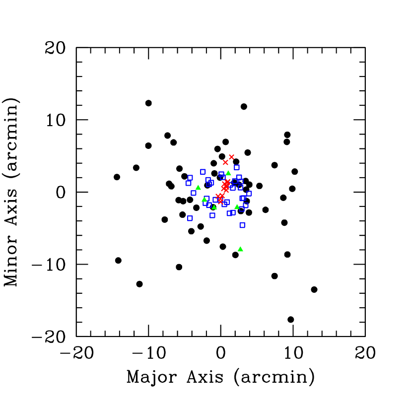
Figure 3: Location of Confirmed M104 GCs. Filled (black) circles: 2dF; Open (blue) squares: WHT; (red) crosses: Keck; Filled (green) triangles: Hydra.

Table 2: Spectroscopically Confirmed M104 Globular Clusters. Successive columns give: ID from RZ04 (where available), ID from B97 or L02 (when applicable), RA, Dec, Radial velocity, Velocity error, Major axis, Minor axis, Galactocentric radius, Azimuthal angle, V, B$-$V, V$-$R, and Source (1=2dF, 2= WHT, 3= Keck, 4= WIYN).

RZ_ID	Other_ID	RA	Dec	Velocity	X	Y	R	$\theta$	V	B$-$V	V$-$R	Source
		(2000)	(2000)	(km/s)	($\arcmin$)	($\arcmin$)	($\arcmin$)	($\deg$)	(mag)	(mag)	(mag)
5319	…	12:39:00.69	-11:35:18.0	1061 $\pm$ 50	-14.38	2.08	14.53	171.79	21.40	0.877	0.577	1
5289	…	12:39:01.43	-11:46:51.0	1092 $\pm$ 58	-14.19	-9.47	17.06	213.73	20.11	0.636	0.467	1
4966	…	12:39:11.62	-11:34:00.6	1047 $\pm$ 26	-11.71	3.37	12.18	163.94	19.73	0.662	0.488	1
4884	…	12:39:13.43	-11:50:06.6	1238 $\pm$ 57	-11.25	-12.73	16.99	228.52	20.60	0.649	0.473	1
4682	…	12:39:18.51	-11:30:57.5	1020 $\pm$ 58	-10.02	6.42	11.90	147.36	20.16	0.684	0.478	1
4679	…	12:39:18.62	-11:25:04.2	1063 $\pm$ 126	-10.00	12.31	15.86	129.10	20.93	0.637	0.487	1
4303	…	12:39:27.74	-11:41:11.7	1070 $\pm$ 31	-7.76	-3.81	8.64	206.18	19.91	0.802	0.516	1
4247	…	12:39:29.37	-11:29:33.3	1019 $\pm$ 47	-7.37	7.82	10.74	133.27	19.65	0.659	0.450	1
4206	…	12:39:30.18	-11:36:13.7	942 $\pm$ 35	-7.16	1.15	7.25	170.86	19.71	0.700	0.457	1
4158	…	12:39:31.48	-11:36:34.9	1285 $\pm$ 119	-6.85	0.80	6.89	173.33	21.37	0.712	0.428	1
4108	…	12:39:32.74	-11:30:31.2	1206 $\pm$ 64	-6.54	6.86	9.48	133.64	20.18	0.735	0.509	1
3987	…	12:39:35.63	-11:38:30.1	1338 $\pm$ 33	-5.83	-1.12	5.93	190.88	19.51	0.664	0.485	1
3974	…	12:39:35.81	-11:47:45.7	1031 $\pm$ 72	-5.78	-10.38	11.88	240.89	20.61	0.683	0.472	1
3965	…	12:39:36.08	-11:34:08.6	1001 $\pm$ 54	-5.72	3.24	6.57	150.48	20.65	0.633	0.445	1
3892	…	12:39:37.77	-11:40:30.7	1136 $\pm$ 32	-5.30	-3.13	6.15	210.56	19.57	0.908	0.580	1
3873	…	12:39:38.14	-11:38:38.5	840 $\pm$ 58	-5.21	-1.26	5.36	193.58	20.16	0.691	0.463	1
3835	…	12:39:38.91	-11:35:12.2	1232 $\pm$ 40	-5.03	2.18	5.48	156.56	20.47	0.655	0.468	1
3728	1-20	12:39:41.19	-11:36:08.3	1186 $\pm$ 51	-4.48	1.23	4.65	164.65	20.69	0.683	0.444	2
3680	…	12:39:41.98	-11:38:27.1	1099 $\pm$ 25	-4.27	-1.07	4.40	194.05	19.47	0.705	0.484	1
3676	2-30	12:39:42.03	-11:40:59.1	1104 $\pm$ 104	-4.28	-3.62	5.60	220.20	21.29	0.965	0.582	2
3667	1-39	12:39:42.14	-11:35:23.4	832 $\pm$ 61	-4.25	1.98	4.69	155.02	21.31	0.831	0.528	2
3638	…	12:39:42.75	-11:42:48.0	987 $\pm$ 45	-4.08	-5.42	6.78	232.98	20.38	0.666	0.475	1
3575	1-25	12:39:44.08	-11:37:29.7	1231 $\pm$ 26	-3.78	-0.12	3.78	181.90	20.75	0.842	0.580	2
3506	…	12:39:45.62	-11:39:33.3	946 $\pm$ 28	-3.38	-2.17	4.02	212.71	19.47	0.960	0.623	1
3461	…	12:39:46.61	-11:36:50.6	1591 $\pm$ 55	-3.14	0.54	3.19	170.25	19.68	1.028	0.579	4
3394	…	12:39:48.09	-11:42:08.4	1330 $\pm$ 31	-2.78	-4.76	5.51	239.72	19.96	0.724	0.470	1
3357	2-12	12:39:49.34	-11:34:34.7	857 $\pm$ 42	-2.49	2.79	3.74	131.69	20.73	0.661	0.457	2
3320	…	12:39:50.13	-11:38:28.9	1259 $\pm$ 113	-2.28	-1.10	2.53	205.76	19.54	0.906	0.554	4
3284	1-32	12:39:50.83	-11:38:54.4	1025 $\pm$ 203	-2.12	-1.54	2.62	216.00	21.11	0.808	0.484	2
3246	…	12:39:51.41	-11:44:06.4	1095 $\pm$ 49	-1.96	-6.72	7.00	253.72	20.60	0.625	0.434	1
3243	2-31	12:39:51.52	-11:38:16.1	939 $\pm$ 21	-1.95	-0.90	2.15	204.69	21.33	0.997	0.628	2
3222	…	12:39:51.89	-11:36:27.1	1162 $\pm$ 30	-1.85	0.93	2.07	153.31	19.89	0.762	0.516	1
3191	2-4	12:39:52.37	-11:35:40.4	968 $\pm$ 78	-1.75	1.69	2.43	135.85	20.41	0.877	0.564	2
3173	1-35	12:39:52.87	-11:39:10.9	1300 $\pm$ 40	-1.62	-1.81	2.43	228.19	21.00	0.661	0.483	2
…	2-16	12:39:52.88	-11:36:17.8	875 $\pm$ 22	-1.62	1.07	1.94	146.50	20.77	0.415	0.303	2
…	2-7	12:39:54.07	-11:36:04.9	976 $\pm$ 24	-1.33	1.29	1.85	135.93	20.52	0.859	0.566	2
3101	1-28	12:39:54.77	-11:40:36.0	932 $\pm$ 25	-1.16	-3.23	3.43	250.29	20.97	0.948	0.593	2
3093	…	12:39:55.07	-11:39:28.6	991 $\pm$ 26	-1.07	-2.09	2.35	242.96	20.28	0.702	0.478	1
3075	…	12:39:55.44	-11:33:24.2	1148 $\pm$ 31	-0.98	3.98	4.10	103.84	19.81	0.717	0.471	1
3064	…	12:39:55.73	-11:39:32.3	972 $\pm$ 102	-0.91	-2.16	2.34	247.21	20.30	0.912	0.557	4
3061	…	12:39:55.84	-11:34:48.4	1007 $\pm$ 30	-0.88	2.58	2.72	108.95	19.46	0.997	0.611	1
…	1-19	12:39:56.45	-11:38:26.0	573 $\pm$ 21	-0.75	-1.07	1.30	234.97	20.71	0.786	0.544	2
2985	…	12:39:57.62	-11:31:25.0	1277 $\pm$ 27	-0.45	5.97	5.98	94.28	19.28	0.916	0.599	1
…	C-136	12:39:58.03	-11:37:59.6	1202 $\pm$ 17	-0.36	-0.58	0.68	238.24	21.79	0.816	0.547	3
2916	…	12:39:58.95	-11:35:22.6	1074 $\pm$ 24	-0.12	2.01	2.01	93.41	19.53	0.735	0.524	1
…	C-132	12:39:59.28	-11:38:21.5	679 $\pm$ 15	-0.05	-0.94	0.94	266.73	20.99	0.871	0.542	3
…	2-8	12:39:59.31	-11:38:27.9	979 $\pm$ 14	-0.05	-1.10	1.10	267.61	20.39	0.918	0.584	2
…	C-137	12:39:59.39	-11:38:46.0	919 $\pm$ 30	-0.02	-1.35	1.35	268.98	21.06	0.926	0.590	3
2877	2-13	12:39:59.82	-11:34:54.6	616 $\pm$ 34	0.08	2.46	2.46	88.17	20.89	0.592	0.487	2
2863	…	12:40:00.16	-11:32:27.7	1300 $\pm$ 29	0.17	4.92	4.92	87.99	19.36	0.835	0.555	1
…	C-116	12:40:00.29	-11:37:54.8	1022 $\pm$ 8	0.19	-0.50	0.54	291.15	20.12	0.716	0.501	3
2832	…	12:40:00.59	-11:44:56.0	1117 $\pm$ 26	0.28	-7.55	7.55	272.16	19.77	0.916	0.599	1
2828	2-6	12:40:00.70	-11:35:19.6	1283 $\pm$ 45	0.29	2.04	2.07	81.80	20.55	0.730	0.497	2
…	C-032	12:40:01.12	-11:36:55.6	1055 $\pm$ 24	0.40	0.48	0.62	50.53	20.60	0.747	0.524	3
2777	2-14	12:40:01.57	-11:39:03.8	1045 $\pm$ 7	0.51	-1.70	1.77	286.72	20.95	0.869	0.557	2
…	C-051	12:40:01.58	-11:36:16.9	1015 $\pm$ 18	0.51	1.13	1.23	65.69	21.30	0.820	0.587	3
2748	…	12:40:02.20	-11:30:26.8	1150 $\pm$ 36	0.67	6.94	6.97	84.45	19.87	0.740	0.479	1
2743	H2-22	12:40:02.26	-11:33:14.1	1274 $\pm$ 17	0.65	4.11	4.16	81.07	18.65	0.566	0.336	3
…	C-042	12:40:02.57	-11:37:08.9	1225 $\pm$ 26	0.75	0.26	0.79	19.25	20.93	0.710	0.516	3
…	C-064	12:40:02.65	-11:36:29.1	865 $\pm$ 16	0.77	0.92	1.20	50.13	21.24	0.673	0.520	3
…	C-059	12:40:02.73	-11:36:42.4	1034 $\pm$ 19	0.79	0.70	1.06	41.67	21.32	0.933	0.566	3
…	2-15	12:40:03.02	-11:38:45.9	828 $\pm$ 71	0.86	-1.40	1.64	301.69	20.90	0.750	0.509	2
…	C-068	12:40:03.21	-11:36:04.4	849 $\pm$ 11	0.90	1.33	1.61	55.80	20.36	0.836	0.549	3
…	C-076	12:40:03.47	-11:35:57.3	1563 $\pm$ 77	0.97	1.45	1.74	56.22	21.51	0.607	0.498	3
2666	…	12:40:03.66	-11:34:50.1	1064 $\pm$ 137	1.04	2.55	2.75	67.86	19.76	0.858	0.547	4
2637	1-26	12:40:04.45	-11:40:18.5	1199 $\pm$ 14	1.21	-2.94	3.18	292.37	20.86	0.914	0.535	2
…	1-11	12:40:04.96	-11:36:21.4	1457 $\pm$ 12	1.34	1.01	1.67	37.07	20.71	0.642	0.450	2
2576	H2-09	12:40:05.65	-11:32:29.5	611 $\pm$ 9	1.50	4.85	5.08	72.86	20.38	0.624	0.469	3
2551	2-2	12:40:06.31	-11:36:47.2	808 $\pm$ 39	1.67	0.58	1.77	19.29	20.40	1.040	0.568	2
2544	2-24	12:40:06.40	-11:40:13.3	1505 $\pm$ 119	1.69	-2.85	3.31	300.57	21.10	0.814	0.526	2
2512	…	12:40:07.08	-11:36:04.7	1189 $\pm$ 27	1.87	1.30	2.28	34.90	19.67	0.920	0.579	1
2491	2-5	12:40:07.50	-11:35:51.5	1220 $\pm$ 89	1.96	1.51	2.47	37.67	20.49	0.751	0.496	2
2475	…	12:40:07.68	-11:46:04.8	1095 $\pm$ 27	2.02	-8.70	8.93	283.07	20.02	0.729	0.457	1
2449	…	12:40:08.09	-11:33:11.1	939 $\pm$ 29	2.12	4.20	4.70	63.24	19.69	0.756	0.526	1
…	2-11	12:40:08.51	-11:33:57.3	1411 $\pm$ 56	2.20	3.41	4.06	57.15	20.89	0.513	0.473	2
2421	…	12:40:08.65	-11:39:30.8	1270 $\pm$ 36	2.26	-2.13	3.10	316.66	19.85	0.917	0.572	4
2363	…	12:40:09.73	-11:36:22.6	1355 $\pm$ 30	2.52	1.01	2.71	21.81	19.45	0.689	0.480	1
2358	1-4	12:40:09.83	-11:35:20.6	1152 $\pm$ 40	2.53	2.03	3.24	38.68	20.51	0.810	0.554	2
2316	…	12:40:10.52	-11:45:20.4	1115 $\pm$ 35	2.71	-7.96	8.41	288.84	20.31	0.864	0.545	4
2307	1-2	12:40:10.67	-11:36:45.3	776 $\pm$ 11	2.73	0.61	2.80	12.64	20.25	0.928	0.542	2
2303	…	12:40:10.77	-11:40:00.6	1207 $\pm$ 34	2.77	-2.63	3.82	316.55	20.02	0.696	0.456	1
2289	1-5	12:40:10.98	-11:35:54.7	755 $\pm$ 61	2.81	1.46	3.17	27.39	20.51	0.577	0.422	2
2257	2-17	12:40:11.38	-11:39:42.9	1275 $\pm$ 100	2.91	-2.35	3.74	321.06	20.82	0.698	0.473	2
2242	1-3	12:40:11.64	-11:38:14.4	1369 $\pm$ 129	2.97	-0.87	3.10	343.65	20.35	0.605	0.440	2
2237	1-15	12:40:11.74	-11:41:56.5	1035 $\pm$ 24	3.00	-4.57	5.47	303.23	20.54	0.698	0.482	2
2200	2-3	12:40:12.45	-11:38:12.1	1524 $\pm$ 14	3.17	-0.83	3.28	345.28	20.44	0.668	0.473	2
2203	…	12:40:12.46	-11:25:33.3	1174 $\pm$ 32	3.19	11.83	12.25	74.92	19.55	0.644	0.479	1
2148	…	12:40:13.48	-11:35:51.3	1136 $\pm$ 35	3.44	1.53	3.76	24.01	20.79	0.713	0.463	1
…	1-29	12:40:13.59	-11:39:12.0	853 $\pm$ 31	3.45	-1.83	3.91	332.02	20.97	1.079	0.672	2
2129	…	12:40:13.79	-11:37:02.4	1167 $\pm$ 62	3.51	0.34	3.53	5.60	19.91	0.751	0.500	1
2109	…	12:40:14.11	-11:38:38.4	1350 $\pm$ 41	3.59	-1.26	3.81	340.74	20.50	0.821	0.539	1
2086	…	12:40:14.64	-11:31:55.5	1063 $\pm$ 23	3.72	5.46	6.61	55.73	19.48	0.718	0.505	1
2038	…	12:40:15.31	-11:40:12.7	1241 $\pm$ 27	3.89	-2.83	4.81	323.97	19.33	0.753	0.487	1
2032	1-16	12:40:15.41	-11:37:34.5	1256 $\pm$ 18	3.90	-0.21	3.90	356.93	20.62	0.874	0.620	2
2021	…	12:40:15.58	-11:36:21.0	1253 $\pm$ 29	3.95	1.03	4.09	14.67	20.19	0.673	0.460	1
1771	…	12:40:21.24	-11:36:31.9	1181 $\pm$ 35	5.34	0.85	5.41	9.07	20.82	0.751	0.507	1
1638	…	12:40:24.74	-11:39:50.7	1072 $\pm$ 51	6.19	-2.46	6.66	338.33	19.56	0.942	0.608	1
1430	…	12:40:29.82	-11:33:40.0	1171 $\pm$ 43	7.44	3.72	8.32	26.55	20.19	0.687	0.474	1
1428	…	12:40:29.82	-11:49:00.2	1056 $\pm$ 42	7.44	-11.62	13.79	302.62	19.67	0.626	0.464	1
1255	…	12:40:34.76	-11:38:10.2	884 $\pm$ 38	8.65	-0.79	8.68	354.80	19.81	0.732	0.508	1
1233	…	12:40:35.37	-11:41:36.6	1230 $\pm$ 52	8.80	-4.23	9.76	334.34	21.41	0.918	0.585	1
1164	…	12:40:36.77	-11:30:25.8	773 $\pm$ 157	9.14	6.95	11.48	37.25	20.46	0.559	0.426	1
1154	…	12:40:37.04	-11:29:27.0	774 $\pm$ 28	9.21	7.93	12.15	40.74	19.44	0.664	0.511	1
1150	…	12:40:37.12	-11:46:01.2	1046 $\pm$ 23	9.22	-8.64	12.63	316.88	19.29	0.740	0.443	1
1070	…	12:40:39.00	-11:55:01.9	1005 $\pm$ 31	9.68	-17.65	20.13	298.74	19.68	0.729	0.484	1
1045	…	12:40:39.82	-11:36:55.1	1025 $\pm$ 26	9.89	0.46	9.90	2.68	19.67	0.759	0.483	1
997	…	12:40:41.23	-11:34:33.0	818 $\pm$ 22	10.23	2.83	10.62	15.48	19.18	0.767	0.538	1
682	…	12:40:52.22	-11:50:52.7	681 $\pm$ 54	12.92	-13.49	18.68	313.75	21.01	0.694	0.440	1

Table 3: Foreground Stars from 2dF and WIYN/Hydra Spectroscopy. Successive columns give: ID from RZ04 (where available), RA, Dec, Radial velocity and error,V, B$-$V, and V$-$R. One object (RZ# 2458) was observed with WIYN/Hydra; all others are from the 2dF data.

4 Results

4.1 Rotation of the Globular Cluster System

The wide field of our study allows us to test for the presence or absence of rotation in the M104 GC system out to 10′ in radius ($\sim$ 30 kpc). In the inner regions, we can compare the results for the GC system to the rotation seen in the stars and gas, while at large radius, our GC data provide a unique probe for rotation in the outer halo of a bulge-dominated galaxy.

Given the strong rotation in the gas and stars in the disk of M104, it is a natural first step to search for rotation along the major axis of the galaxy. In Figure 4 we plot radial velocity vs. major axis distance for the 108 GCs in our sample. It is immediately apparent from this figure that the GC system has little rotation along the major axis, in contrast to the large rotation seen in the stars and gas along the disk on the major axis. This rotation from major axis measurements of stars and gas is shown as the dotted line, where the inner points to $r\simeq 0.7^{\prime}$ are from the stellar absorption line measurements of van der Marel et al. (1994) and the line beyond this from the fit of Kormendy & Westpfahl (1989) to a number of observations of HII regions and HI gas, which have their farthest extent at $r\simeq 3^{\prime}$.

The smoothed velocity profile for the GC sample is shown in Figure 4 as the dashed line, where the velocities have been smoothed using a Gaussian kernel with a width of $\sigma=3^{\prime}$. This confirms the strong visual impression that there is no clear rotation in the GC sample out to large radii. Based on a smaller dataset at $r<5.5\arcmin\$, B97 presented a tentative detection of rotation (at a confidence level of 92.5%), that is not found in our more extensive work here. Figure 4 also shows that the metal-rich and metal-poor GCs are similar in their weak or absent rotation. There is a hint of counter-rotation or asymmetry in the velocity profile at very large radius, but spectroscopic data for significantly more outer GCs will be required to test any such effect. The dominant conclusion from the GC data is that there is no significant rotation over the large range of radii studied, and any rotation that might be present is much smaller than the observed rotation of stars and gas along the major axis.

We can also extend our search for rotation to all possible position angles. Figure 5 plots radial velocity vs. azimuthal angle for all 108 M104 GCs. Figure 5 shows that there is no obvious rotation about any position angle in the M104 GC system. To quantify this result, we have performed non-linear least squares fits to this equation: V($\theta$) = V_rotsin($\theta$ - $\theta_{0}$) + V₀, where $V_{rot}$ is the rotation amplitude, $\theta$ is the azimuthal angle ($\theta$ = 0 corresponds to the positive branch of the major axis, and East on the sky), and $V_{0}$ is the systemic velocity of M104. This corresponds to determining the best-fitting flat rotation curve (see Zepf et al. 2000 for more details).

We carried out this test for rotation about any axis in the total GC sample, and also in sub-samples split by colour and galactocentric radius. Our colour boundary is set at (B$-$R) = 1.3 (see Section 3), while we divide by radius at 5′ ($\sim$ 15 kpc). Columns 2 & 3 of Table 4 give the best-fit rotation velocity and position angle returned by the least-squares code. We have assessed the significance of these rotation velocities through Monte-Carlo simulations which keep the GC azimuthal angles but randomize the velocities (cf. Zepf et al. 2000); the significance level is defined as the fraction of simulations with rotation velocity lower than the best-fit rotation velocity. As can be seen from Column 4 of Table 4, there is no significant rotation seen in any of the GC sub-samples. We have also used Monte Carlo simulations to set upper limits on the rotation velocity. We do this by generating artificial samples with the same position angle distributions and velocity dispersions as the data, with a rotation curve of given amplitude imposed. The 95% confidence upper limit is defined as the rotation velocity for which only 5% of these simulations give a rotation velocity as small as that observed (see Zepf et al. 2000); this upper limit is given in Column 5 of Table 4. We then use these values, together with the measured velocity dispersion of each sample (Column 6), to determine upper limits for (v/$\sigma$), which measures the importance of rotation in a dynamical system. Our (v/$\sigma$) upper limits, given in the 7th Column of Table 4, range from 0.5 to 1.6.

The lack of rotation seen in the M104 GC system is surprising. Given the edge-on alignment of M104’s disk, it is difficult to argue that there is rotation in the GC system but that we are viewing it face-on. Cosmological simulations predict that early-type galaxies have significant amounts of angular momentum (e.g. Vitvitska et al. 2002). The stellar and gas disk clearly has some angular momentum (Figure 4), but the disk is only 10% of the total $B$ light (Burkhead 1986), and less by mass, and cannot account for the expected overall angular momentum. There would seem to be two options: that some luminous spheroid-dominated galaxies have less angular momentum than expected from hierarchical merging; or that angular momentum has been transferred to even larger radius by mergers during the formation of M104 (e.g. Hernquist & Bolte 1993). Given the long-standing and consistent predictions for the angular momentum content of galaxies, the latter option of angular momentum transport through merger-like processes would seem to be favoured. The absence of evidence for recent activity in M104 from either GC ages (L02; Hempel et al. 2006) or other measures would suggest these processes happened in M104 a number of Gyr ago, corresponding to redshifts greater than one or two. Interestingly, the M104 bulge planetary nebulae (PNe) show spheroidal rotation– between a radius of 1$-$4′, the PNe rotation is $\sim$ 100 km/s near the equatorial plane, and decreasing away from the plane (K. Freeman, unpublished data). The PNe rotation, coupled with the lack of rotation in the GC system, show that these two populations are dynamically quite distinct, and presumably formed in very different ways. We plan to obtain more GC velocities at very large radii to further investigate these issues.

Figure 4: Radial velocity vs major axis distance for M104 GCs. Circles are blue GCs (B$-$R $<$ 1.3), and triangles are red GCs (B$-$R $>$ 1.3). The dashed line is a smoothed fit to the GC velocities, while the dotted line shows the stellar and gas rotation curve from van der Marel et al. (1994) and Kormendy & Westpfahl (1989).

Table 4: Rotation analysis for M104 GCs. Column 1 gives the sample under consideration, Column 2 the least-squares fit for the rotation velocity, Column 3 the position angle for this fit, Column 4 the significance of this fit, Column 5 the 95% upper limit on the rotation velocity, Column 6 the velocity dispersion, and Column 7 the 95% upper limit on (v/$\sigma$).

Sample	Vrot	$\theta_{0}$	Significance	V${}^{max}_{rot}$ (95%)	$\sigma$	(v/$\sigma$) (95%)
	(km/s)	(deg)	(%)	(km/s)	(km/s)
All clusters (N=108)	60	-41	35	100	204	0.49
(B$-$R $<$ 1.3) (N=66)	120	-38	36	175	203	0.86
(B$-$R $>$ 1.3) (N=42)	30	35	13	100	207	0.48
R $<$ 5′ (N=65)	82	7	57	140	233	0.60
R $>$ 5′ (N=43)	198	60	81	250	155	1.61

Figure 5: Radial velocity vs azimuthal angle for M104 GCs. There is no clear rotation seen in the M104 GC system.

4.2 Globular Cluster Velocity Dispersion Profile

The large radial extent of our GC sample also allows us to probe the velocity dispersion profile of the M104 GC system from the inner region well out into the distant halo. This dispersion profile can then be combined with the observed spatial profile of the GC system and assumptions about the GC orbits to derive the mass distribution of M104 over a large radial range. To display the data, we plot in the top panel of Figure 6 V$-$V_M104 against projected radius R for our 108 M104 GCs. Note that the mean velocities for GCs with R $<$ 5′ (65 GCs) and R $>$ 5′ (43 GCs), 1099 $\pm$ 28 and 1058 $\pm$ 25 km/s respectively, agree with the mean velocity for all GCs (1083 $\pm$ 20 km/s). To enable any rotation to be made clear, we have flipped the sign of the offset for GCs to the west of the galaxy center (those with negative $r_{maj}$ in Figure 4). Thus the overall consistency of the offset velocities with zero in Figure 6 is further evidence for the absence of rotation discussed earlier. The exception to this may be for R $>$ $\sim$ 10′, where most of the points have V$-$V_M104 $<$ 0 (effectively counter-rotating with respect to the stars and gas in the inner galaxy). As mentioned in the previous section, more data will be required to obtain a definitive result on this issue.

The top panel of Figure 6 suggests that the velocity dispersion of the M104 GCs declines with projected radius, with the impression that it is fairly high inside of $\sim 5^{\prime}$, then declines fairly steeply, and possibly flattens at large radii. We first quantify this by dividing our sample into an inner and an outer bin, with a somewhat arbitrary division at R=5′. The dispersions in these two regions are $\sigma$(R$<$5′) = 233 $\pm$ 20 km/s, and $\sigma$(R$>$5′) = 155 $\pm$ 28 km/s. We can also make a continuous estimate of the velocity dispersion with radius by smoothing the individual GC velocities. In addition to avoiding issues of binning, this calculation of the smoothed velocity dispersion profile allows the mass distribution to be determined. The bottom panel of Figure 6 shows the smoothed velocity dispersion profile vs. projected radius $R$ for our M104 dataset. The smoothing is done with a Gaussian kernel with a width that slowly increases from $\sigma$ = 2′ in the center to $\sigma$ = 2.5′ in the outer region, and the uncertainties in the dispersion estimate are based on a bootstrap technique accounting for the kernel used (cf. Zepf et al. 2000). The upper and lower dotted lines correspond respectively to the $1\sigma$ upper and lower limits for the velocity dispersion at that radius. We have not corrected our velocity dispersions for measurement errors; these corrections would change the velocity dispersion by less than 10% everywhere, except perhaps at the very largest radii if the true dispersion is very low and the typical measurement uncertainties are at the upper end of published estimates. The binned results discussed above are plotted as open circles with error bars, where the points are plotted at the $R$ corresponding to the median distance of the GC sample in each bin from the galaxy center.

The primary result from this analysis is that the dispersion is about 230 km/s within the central few arcmin (recall that $R_{e}$ = 105″ or 5 kpc), and then begins to decline fairly steeply at around $5^{\prime}$, and then possibly flattens at larger radii, although our data are too sparse at very large radii (e.g. $R\sim 15\arcmin$ or $\sim 45$ kpc) to tell. A key use of this dispersion profile is for estimating the mass of M104 through the Jeans equation, which we do in the following section.

Figure 6: Top: V $-$ V_M104 vs. projected radius R for M104 GCs ($R$). Metal-rich GCs are plotted as triangles and metal-poor as circles, as in Figure 4. The dotted horizontal lines show the mean velocity for inner $(R<5^{\prime})$ and outer $(R>5^{\prime}$) samples, while the solid vertical lines indicate the velocity dispersion for each of these subsamples. We adopt a systemic velocity V_M104 = 1083 km/s, the mean velocity for all GCs. The radial extent of this figure is about 60 kpc (12 $R_{e}$). Bottom: Smoothed velocity dispersion profile for M104 GCs. The upper and lower dotted lines represent the $1\sigma$ limits for the velocity dispersion. The open circles with error bars are the dispersions in the two bins mentioned above, plotted at the median radius of each of the bins. This plot shows the declining velocity dispersion profile seen in our data.

4.3 The Mass Distribution of M104

The velocity dispersion profile determined above can be combined with the previously published spatial profile of the GC system (RZ04) and the Jeans equation to determine the mass distribution of M104. The large radial range of our GC velocity data allows us to compare the mass estimate from the GCs with other tracers out to a few arcminutes, and then to extend the estimate of the mass distribution much farther into the halo of M104. This calculation of the mass distribution from the Jeans equation is straightforward with the assumptions of isotropy and spherical symmetry. Spherical symmetry is supported at least outside the central regions by the round isophotes of M104 (e.g. Burkhead 1986). Isotropy for the GC orbits in ellipticals is supported by all cases in which an independent constraint on the mass distribution from X-ray observations is available (e.g. M49: Zepf et al. 2000, Côté et al. 2003; M87: Côté et al. 2001; M60: Bridges et al. 2006), although the metal-poor and metal-rich GCs in these galaxies often show differences from isotropy when considered separately. Moreover, for our work on M104, we can test the mass distribution with these assumptions directly against the mass inferred from the rotation curve measured out to $r\leq 3^{\prime}$.

The mass distribution resulting from the Jeans equation calculation, using the GC velocity dispersion profile found here and the best-fitting R^1/4-law profile for the GC surface density distribution from RZ04, is shown in the top panel of Figure 7. We have imposed a cutoff in the GC surface density profile at 15′ (projected) radius, consistent with RZ04, but we have checked that cutoff radii of 30′ or 60′ only change the mass profile by a few percent between 1$-$9.5′ (deprojected) radius. In Figure 7, the upper and lower lines are the $1\sigma$ upper and lower limits on the mass (top) and (M/L)_V (bottom). These are based on the bootstrapped uncertainties of the velocity dispersion profile, which dominate over any uncertainty in the density profile of the GC system. The dashed line at small radii is the mass inferred from the rotation curve fit given by Kormendy & Westpfahl (1989), based on their analysis of a variety of data in the literature. The mass profiles inferred from the isotropic Jeans equation for our GC sample and from the rotation seen in the disk are in excellent agreement. This agreement suggests that deviations from the assumptions in the Jeans equation analysis, such as the known ellipticity of the isophotes in the central regions (e.g. Burkhead 1986) and/or any anisotropy, produce only modest changes in the mass distribution which are less than the given uncertainties. In Appendix A, we tabulate L_V(r) and the 1$\sigma$ limits for M(r) and (M/L)_V(r).

The mass profile inferred from the GC kinematics in Figure 7 continues to rise roughly linearly with radius from the inner regions to at least $7^{\prime}$ ($\sim$ 20 kpc), after which it begins to level off. This naturally follows from the dispersion profile in Figure 6 which is approximately constant to about this radius accounting for projection, and then falls in an almost Keplerian way at larger radii. The roughly linear rise in the enclosed mass from about $\sim 0.5$ to $\sim 4$ $R_{e}$ ($R_{e}$ = 105″ or 5 kpc) is solid evidence of a dark matter halo around M104. To show this more explicitly, in the bottom panel of Figure 7 we plot the V-band mass-to-light ratio against deprojected radius r for M104. This is derived directly from the mass profile in the top panel and the deprojected V-band luminosity profile from Kormendy & Westpfahl (1989). This luminosity profile agrees to within 5% with our analysis of the Mosaic CCD data of RZ04, and is also in agreement with other previously published work (e.g. Burkhead 1986).

The radial dependence of the mass-to-light ratio of M104 plotted in Figure 7 has two major features: a rise in the $(M/L)_{V}$ ratio from a value of $\sim$ 4 at $r=0.7^{\prime}$ to a value of $\sim$ 17 at $r=7^{\prime}$ ($\sim$ 20 kpc, or 4 R_e), and a flattening in M/L beyond 7′. We discuss each of these in turn. There seems to be no way to account for the rise in M/L except for a significant dark matter halo around M104. There is no evidence for a change in the stellar population of the galaxy over this radial range, as the colors show little or no change over this region, and in any case, it is hard to imagine how to produce such a large M/L change in a red spheroidal population. The increase in M/L from r = $0.7^{\prime}-7^{\prime}$ is also too large to be easily explained by an orbital structure which changes with radius. Moreover, the comparison with the rotation curve supports isotropy for the GC orbits in the inner half, and it would seem contrived for the orbits to suddenly become more tangential just at the point where the rotation curve measurements end.

Thus the data strongly support the presence of a dark matter halo in M104. One can also use this analysis to place some broad constraints on the properties of this dark matter halo. We can use our results to estimate the fraction of dark matter at one $R_{e}$ (105″, or 5 kpc). To do this, we note that even the upper limit for the mass-to-light ratio at $0.7^{\prime}$ of $M/L_{V}=5.3$ is not larger than the $M/L_{V}$ of models of stellar populations with red colours like the M104 halo. Specifically, this $M/L_{V}$ is less than expected from models with a Salpeter IMF down to $0.1M_{\odot}$, and within the range of models with fewer low-mass stars than Salpeter, such as the IMF of Chabrier (2003). We discuss this further below, but here note that this suggests that the mass at 0.7′ has little dark matter contribution. Setting the $M/L_{V}$ value at $r\sim 0.7^{\prime}$ as the stellar value and using the absence of a significant color gradient as evidence that this applies out to large radii, we can then compute the mass fraction of dark matter required to account for the mass at one $R_{e}$. When we do this, we find a dark matter fraction at one R_e of 19%. This fraction would increase somewhat if the mass at 0.7′ was not completely dominated by stars. We also note that depending on the exact choice of stellar M/L, the halo may be isothermal or somewhat shallower in density profile over the radial range of $0.7^{\prime}-7^{\prime}$, corresponding approximately to $2-20$ kpc or $0.4-4$ R_e. This is consistent with findings of close to isothermal mass profiles from strong lensing (Rusin et al. 2003, Treu & Koopmans 2004) over a radial range encompassed by this study.

Our data also allow us to note that at $2R_{e}$ the dark matter fraction of the mass is about $49\%$ and at $5R_{e}$ it has risen to about $75\%$. M104 thus provides a strong argument against proposals in which early-type galaxies are either strongly baryon or dark matter dominated around one R_e: instead we find a mix. While a wide range of possibilities has been stated at various times in the literature, this result is in good agreement with the kinematic studies of the integrated light of elliptical galaxies (e.g. Gerhard et al. 2001), as well as the strong lensing studies of a few more distant galaxies noted above (Treu & Koopmans 2004).

We note that the $(M/L)_{V}$ inferred in our analysis at $\sim$ 0.7′ (0.4 R_e) is in the range $3-5$. We can compare this mass-to-light ratio with those obtained from stellar population models consistent with the observed colours of the halo of M104. For $(B-V)\simeq 0.95$, found by both Burkhead (1986) and our own Mosaic data, stellar population models with a Salpeter IMF give significantly higher mass-to-light ratios than observed. M104’s disk does not affect the result significantly, as the disk makes up only about $10\%$ of the light; thus, even if one assumes the disk contributes no mass, the correction to the M/L ratio is not significant. The same result is found when using any of the current stellar population models (e.g. Vazdekis et al. 1996, Bruzual & Charlot 2003, Maraston 2005). The conclusion then is that the mass-to-light ratio at $\sim 0.4R_{e}$ indicated by both GC velocities and the galaxy rotation curve requires fewer low-mass stars well below the turnoff than given by a Salpeter IMF extended to $0.1M_{\odot}$. Similar conclusions have been drawn from other studies of the central regions of elliptical galaxies (e.g. Cappellari et al. 2006), and the suggestion of an IMF with fewer low-mass stars than Salpeter has a long history in both elliptical (e.g. Larson 1986, Zepf & Silk 1996) and spiral (Bell & de Jong 2001) galaxies.

Our kinematic data extend well beyond the $\sim$ 20 kpc above, with our most distant point at $\sim$ 60 kpc. Although our dispersion profile becomes too uncertain at these largest radii to reasonably constrain the mass profile, our data do show a drop in the velocity dispersion outside $\sim$ 20 kpc (Figure 6). Our best fit is that this drop in dispersion is steep enough to be nearly Keplerian, and thus the simplest interpretation of the enclosed mass profile is that there is little mass beyond this radius. This can be seen in the mass profile at large radii in Figure 7. This apparent flattening of the mass profile beyond 20 kpc radius is not affected by the radial extent of the GC surface density profile adopted; as noted above, the mass profile only changes by a few percent for cutoff radii of 15′, 30′, or 60′. However, there are viable alternatives to the conclusion that the dark matter halo does not extend much beyond 20 kpc. The most obvious issue is whether the assumption of isotropic orbits holds at these larger radii or whether the orbits become more radial, which would reconcile the low dispersion estimate with a higher mass. Another possibility is that the low velocity dispersion is simply a several sigma fluctuation. Both of these can be addressed with significantly more GC velocities at larger radii from the center of M104. Fortunately, there are GCs to be observed at these distances (e.g. RZ04), so the study of the dark matter halo of M104 can be pushed to yet larger radii.

Figure 7: Top: Mass vs deprojected radius r for M104. The solid lines give the 1$\sigma$ bounds for the mass profile as determined from the GCs, while the dotted line gives the mass profile determined from the stellar rotation curve (Kormendy & Westpfahl 1989). Bottom: M/L_V vs deprojected radius r for M104. The mass profile is taken from the top plot, while the luminosity profile is taken from the Mosaic CCD data of RZ04. A galaxy without a dark matter halo, in which mass traces light, would show a flat line in this plot.

5 Conclusions

We have obtained new velocities for 62 globular clusters (GCs) in M104, 56 of these with 2dF on the AAT and 6 with Hydra on WIYN. Combined with previous data from Bridges et al. (1997) and Larsen et al. (2002), we have a total sample of 108 GC velocities, making M104 one of the few galaxies with more than 100 GC velocities. Our data extend out to 20′ ($\sim$ 60 kpc) in galactocentric radius, allowing us to study M104 well out into its halo. Our main conclusions are as follows:

1. We see no evidence for rotation in the GC system. This is true for the entire GC system, and also for subsets split by colour and galactocentric radius. This lack of rotation is particularly interesting, because there is rotation of 300$-$350 km/s in the stellar and gas disk (van der Marel et al. 1994; Kormendy & Westpfahl 1989), and cosmological simulations of galaxy formation predict significant amounts of angular momentum in early-type galaxies. A possible resolution is that galaxy mergers transport angular momentum to large radii during the formation of early-type galaxies. There is a suggestion that the GCs counter-rotate with respect to the stars and gas at large radius. We plan to obtain GC velocities to even larger radii in M104 to better quantify the rotation in the GC system.

2. The GC velocity dispersion is 200$-$250 km/s within $\sim$ 3′ of the galaxy center, but then drops to $\sim$ 150 km/s at 10′, and possibly flattens at larger radii.

3. Using our GC dispersion profile and the GC spatial profile from RZ04, together with the Jeans equation assuming isotropy and spherical symmetry, we determine the mass distribution of M104 out to $\sim$ 10′ radius ($\sim$ 30 kpc). There is excellent agreement between the mass profile derived from the GCs and the profile inferred from the rotation curve fit of Kormendy & Westpfahl (1989) out to 3′ radius, supporting our assumption of isotropy in the GC system.

   Our mass profile rises roughly linearly with radius out to about 7′ ($\sim$ 20 kpc), beyond which it levels off. The M/L_V increases from $\sim$ 4 at r = 0.7′ to $\sim$ 17 at r=7′ (20 kpc, or 4 R_e). It seems difficult to attribute the increase in M/L to changes in either the stellar population or GC anisotropy with radius. The data thus strongly support the presence of a dark matter halo in M104. We find that dark matter contributes $\sim$ 20% of the total mass within one effective radius, which is in agreement with studies of the integrated light of elliptical galaxies, and strong lensing studies of more distant galaxies.

4. We find a M/L_V of 3$-$5 at 0.4 R_e, which is difficult to explain with stellar population models assuming a Salpeter IMF down to 0.1 M_⊙. This M/L_V can be accounted for by an IMF with fewer low mass stars than Salpeter, which has also been found in many other environments including the Milky Way and other early-type galaxies.

5. More GC velocities, particularly at large radius, will tighten our interesting constraints on the rotation and the velocity dispersion/mass profile of the M104 GC system. It would be very interesting to carry out a detailed comparison of GC and planetary nebulae velocities, in order to test for similarities or differences between the orbital properties of these two populations.

Appendix A Appendix A

In this Appendix, we present in tabular form the luminosity and mass profiles plotted in Figure 7. The enclosed V-band L_V(r) profile was determined from the Mosaic images of M104 discussed in Rhode & Zepf (2004), supplemented by an analysis of images from the Hubble Space Telescope in the very central regions where the Mosaic data were saturated. The enclosed mass profiles M(r) were derived as discussed in the text, with the upper and lower M(r) representing the $1\sigma$ confidence limits. (M/L)_V(r) is simply M(r)/L(r), with upper and lower values again representing $1\sigma$ confidence limits.

The full version of Table 5 is available in the ApJ online edition of this paper, or by request from T. Bridges

Table 5: Enclosed luminosity, mass, and mass-to-light ratio versus deprojected radius r for M104. Column 1: radius in arcmin; Column 2: enclosed luminosity in solar units; Columns 3&4: lower and upper 1$\sigma$ confidence limits on the enclosed mass in solar units; Columns 5&6: lower and upper 1$\sigma$ confidence limits on the (M/L)_V.

References

- Ashman & Zepf (1992) Ashman, K.M., & Zepf, S.E. 1992, ApJ, 384, 50
- Ashman & Zepf (1998) Ashman, K.M., & Zepf, S.E. 1998, Globular Cluster Systems (Cambridge: Cambridge University Press)
- Barbier-Brossat et al. (1994) Barbier-Brossat, M., Petit, M., & Figon, P. 1994, A&AS, 108, 603
- Barbier-Brossat & Figon (2000) Barbier-Brossat, M., & Figon, P. 2000, A&AS, 142, 217
- Beers et al. (1990) Beers, T.C., Flynn, K., & Gebhardt, K. 1990, AJ, 100, 32
- Bell & de Jong (2001) Bell, E.F., & de Jong, R.S. 2001, ApJ, 550, 212
- Bridges & Hanes (1992) Bridges, T.J., & Hanes, D.A. 1992, AJ, 103, 800
- Bridges et al. (1997) Bridges, T.J., Ashman, K.M., Zepf, S.E., Carter, D., Hanes, D.A., Sharples, R.M., & Kavelaars, J.J. 1997, MNRAS, 284, 376 [B97]
- Bridges et al. (2006) Bridges, T.J., Gebhardt, K., Sharples, R., Faifer, F.R., Forte, J.C., Beasley, M.A., Zepf, S.E., Forbes, D.A., Hanes, D.A., & Pierce, M. 2006, MNRAS, in press
- Brodie & Strader (2006) Brodie, J.P., Strader, J. 2006, ARA&A, in press (astroph/0602601)
- Bruzual & Charlot (2003) Bruzual, G., & Charlot, S. 2003, MNRAS, 344, 1000
- Burkhead (1986) Burkhead, M.S. 1986, AJ, 91, 777
- Cappellari et al. (2006) Cappellari, M., Bacon, R., Bureau, M., Damen, M.C., Davies, R.L., de Zeeuw, P.T., Emsellem, E., Falcon-Barroso, J., Krajnovic, D., Kuntschner, H., McDermid, R.M., Peletier, R.F., Sarzi, M., van den Bosch, R.C.E., & van de Ven, G. 2006, MNRAS, 366, 1126
- Chabrier (2003) Chabrier, G. 2003, ApJ, 586, L133
- Cohen (2000) Cohen, J.G. 2000, AJ, 119, 162
- Côté et al. (2001) Côté, P., McLaughlin, D.E., Hanes, D.A., Bridges, T.J., Geisler, D., Merritt, D., Hesser, J.E., Harris, G.L.H., & Lee, M.G. 2001, ApJ, 559, 828
- Côté et al. (2003) Côté, P., McLaughlin, D.E., Cohen, J.G., & Blakeslee, J.P. 2003, ApJ, 591, 850
- Croom et al. (2005) Croom, S., Saunders, W., Heald, R., & Bailey, J., “The 2dfdr Data Reduction System Users Manual, available at www.aao.gov.au/AAO/2df/manual.html
- Dekel et al. (2005) Dekel, A., Stoehr, F., Mamon, G.A., Cox, T.J., Novak, G.S., & Primack, J.R. 2005, Nature, 437, 707
- de Vaucouleurs et al. (1991) de Vaucouleurs, G., de Vaucouleurs, A., Corwin, H.G., Buta, R.J., Paturel, G., & Fouque, P. 1991, “Third Reference Catalogue of Bright Galaxies”, Springer-Verlag
- Faber et al. (1977) Faber, S.M., Balick, B., Gallagher, J.S., & Knapp, G.R. 1977, ApJ, 214, 383
- Forbes et al. (1997) Forbes, D.A., Brodie, J.P., & Grillmair, C.J. 1997, AJ, 113, 1652
- Gebhardt & Kissler-Patig (1999) Gebhardt, K. & Kissler-Patig, M. 1999, AJ, 118, 1526
- Ford et al. (1996) Ford, H.C., Hui, X., Ciardullo, R., Jacoby, G.H., & Freeman, K.C. 1996, ApJ, 458, 455
- Gerhard et al. (2001) Gerhard, O., Kronawitter, A., Saglia, R.P., & Bender, R. 2001, AJ, 121, 1936
- Harris & van den Bergh (1981) Harris, W.E., & van den Bergh, S. 1981, AJ, 86, 1627
- Harris et al. (1984) Harris, W.E., Harris, H.C., & Harris, G.L.H. 1984, AJ, 89, 216
- Harris (1996) Harris, W.E. 1996, AJ, 112, 1487
- Harris & van den Bergh (1981) Harris, W.E. & van den Bergh, S. 1981, AJ, 86, 1627
- Hempel et al. (2006) Hempel, M., Zepf, S.E., Kundu, A., Geisler, D., & Maccarone, T.J. 2006, in preparation
- Hernquist & Bolte (1993) Hernquist, L., & Bolte, M. 1993, in “The Globular Clusters-Galaxy Connection”, ASP Conference Series #48, ed. G.H. Smith & J.P. Brodie, pg. 788
- Kent (1988) Kent, S.M. 1988, /aj, 96, 514
- Kormendy & Westpfahl (1989) Kormendy, J., & Westpfahl, D.J. 1989 ApJ, 338, 752
- Kronawitter et al. (2000) Kronawitter, A., Saglia, R.P., Gerhard, O., & Bender, R. 2000, A&AS, 144, 53
- Kundu & Whitmore (2001) Kundu, A. & Whitmore, B.C. 2001, AJ, 121, 2950
- Larsen et al. (2001) Larsen, S.S., Forbes, D.A., & Brodie, J.P. 2001, MNRAS, 327, 1116
- Larsen et al. (2002) Larsen, S.S., Brodie, J.P., Beasley, M.A., & Forbes, D.A. 2002, AJ, 124, 828 [L02]
- Larson (1986) Larson, R.B. 1986, MNRAS, 218, 409
- Lewis et al. (2002) Lewis, I.J., Cannon, R.D., Taylor, K., Glazebrook, K., Bailey, J.A., Baldry, I.K., Barton, J.R., Bridges, T.J., Dalton, G.B., Farrell, T.J., Gray, P.M., Lankshear, A., McCowage, C., Parry, I.R., Sharples, R.M., Shortridge, K., Smith, G.A., Stevenson, J., Straede, J.O., Waller, L.G., Whittard, J.D., Wilcox, J.K., & Willis, K.C. 2002, MNRAS, 333, 279
- Malaroda et al. (2001) Malaroda, S., Levato, H., & Galliani, S. 2001, VizieR On-line Data Catalog: III/216
- Maraston (2005) Maraston, C. 2005, MNRAS, 362, 799
- Monet et al. (1998) Monet, D., Bird, A., Canzian, B., Dahn, C., Guetter, H., Harris, H., Henden, A., Levine, S., Luginbuhl, C., Monet, A.K.B., Rhodes, A., Riepe, B., Sell, S., Stone, R., Vrba, F., & Walker, R. 1998, “The USNO-A2.0 Catalogue”, VizieR On-Line Data Catalog: I/252, US Naval Observatory
- Peng et al. (2004) Peng, E.W., Ford, H.C., & Freeman, K.C. 2004, ApJ, 602, 705
- Perrett et al. (2002) Perrett, K.M., Bridges, T.J., Hanes, D.A., Irwin, M.J., Brodie, J.P., Carter, D., Huchra, J.P., & Watson, F.G. 2002, AJ, 123, 2490
- Petrov et al. (2006) Petrov, L., Kovalev, Y.Y., Fomalont, E.B., & Gordon, D. 2006, AJ, 131, 1872
- Rhode & Zepf (2001) Rhode, K.L. & Zepf, S.E. 2001, AJ, 121, 210
- Rhode & Zepf (2004) Rhode, K.L. & Zepf, S.E. 2004, AJ, 127, 302 [RZ04]
- Richtler et al. (2004) Richtler, T., Dirsch, B., Gebhardt, K., Geisler, D., Hilker, M., Alonso, M.V., Forte, J.C, Grebel, E.K., Infante, L., Larsen, S., Minniti, D., & Rejkuba, M. 2004, /aj, 127, 2094
- Roberts & Haynes (1994) Roberts, M.S., & Haynes, M.P. 1994, ARA&A, 32, 115
- Rubin et al. (1978) Rubin, V.C., Thonnard, N., & Ford, W.K. 1978, ApJ, 225, 107
- Rusin et al. (2003) Rusin, D., Kochanek, C.S., & Keeton, C.R. 2003, ApJ, 595, 29
- Schlegel, Finkbeiner, & Davis (1998) Schlegel, D., Finkbeiner, D., & Davis, M. 1998, ApJ, 500, 525
- Spitler et al. (2006) Spitler, L.R., Larsen, S.S., Strader, J., Brodie, J.P., Forbes, D.A., & Beasley, M.A. 2006, AJ, in press (astroph/0606337)
- Tonry et al. (2001) Tonry, J.L., Dressler, A., Blakeslee, J.P., Ajhar, E.A., Fletcher, A.B., Luppino, G.A., Metzger, M.R., & Moore, C.B. 2001, ApJ, 546, 681
- Treu & Koopmans (2004) Treu, T., & Koopmans, L.V.E. 2004, ApJ, 611, 739
- van der Marel et al. (1994) van der marel, R.P., Rix, H.-W., Carter, D., Franx, M., White, S.D.M., & de Zeeuw, T. 1994, MNRAS, 268, 521
- Vazdekis et al. (1996) Vazdekis, A., Casuso, E., Peletier, R.F., & Beckman, J.E. 1996, ApJS, 106, 307
- Vitvitska et al. (2002) Vitvitska, M., Klypin, A.A., Kravtsov, A.V., Wechsler, R.H., Primack, J.R., & Bullock, J.S. 2002, ApJ, 581, 799
- Zepf et al. (2000) Zepf, S.E., Beasley, M.A., Bridges, T.J., Hanes, D.A., Sharples, R.M., Ashman, K.M., & Geisler, D. 2000, AJ, 120, 2928
- Zepf & Silk (1996) Zepf, S.E. & Silk, J. 1996, ApJ, 466, 114