The usage of Strömgren photometry in studies of Local Group Dwarf Spheroidal Galaxies

Abstract

Aims. In this paper we demonstrate how Strömgren $uvby$ photometry can be efficiently used to: 1. Identify red giant branch stars that are members in a dwarf spheroidal galaxy. 2. Derive age-independent metallicities for the same stars and quantify the associated errors.

Methods. Strömgren $uvby$ photometry in a 11 $\times$ 22 arcmin field centered on the Draco dwarf spheroidal galaxy was obtained using the Isaac Newton Telescope on La Palma. Members of the Draco dSph galaxy were identified using the surface gravity sensitive $c_{1}$ index which discriminates between red giant and dwarf stars. Thus enabling us to distinguish the (red giant branch) members of the dwarf spheroidal galaxy from the foreground dwarf stars in our galaxy. The method is evaluated through a comparison of our membership list with membership classifications in the literature based on radial velocities and proper motions. The metallicity sensitive $m_{1}$ index was used to derive individual and age-independent metallicities for the members of the Draco dSph galaxy. The derived metallicities are compared to studies based on high resolution spectroscopy and the agreement is found to be very good.

Results. We present metallicities for 169 members of the red giant branch in the Draco dwarf spheroidal galaxy (the largest sample to date). The metallicity distribution function for the Draco dSph galaxy shows a mean [Fe/H] = –1.74 dex with a spread of 0.24 dex. The correlation between metallicity and colour for the stars on the red giant branch is consistent with a dominant old, and coeval population. There is a possible spatial population gradient over the field with the most metal-rich stars being more centrally concentrated than the metal-poor stars.

1 Introduction

When first discovered, dwarf spheroidal galaxies (dSph) were considered similar to the Galactic globular clusters because of their old stellar populations and apparent lack of gas (Shapley 1938; Hodge 1971). Over the years this picture has changed. It is today known that dSphs show complex features like large variations in their star formation histories and metallicities (e.g. Mateo 1998 and references therein, Shetrone et al. 2001a; Dolphin 2002). A large fraction of the dSphs also show population gradients with a concentration of the more metal-rich stars in the central regions (e.g. Harbeck et al. 2001).

The Draco dSph galaxy is one of the faintest companions to our galaxy, the Milky Way, with a total luminosity of 2 $\times 10^{5}{\rm L_{\odot}}$ (Grillmair et al. 1998) and it lies in close proximity to the Milky Way with a distance of $\sim$ 82 kpc (Mateo 1998). A large number of photometric and spectroscopic investigations have been aimed at the Draco dSph galaxy and it is today clear that while the star formation history shows a predominately old population (Grillmair 1998; Dolphin 2002) there exists an internal metallicity spread in the dwarf spheroidal galaxy (e.g. Zinn 1978, 1980; Bell et al. 1985; Carney & Seitzer 1986; Shetrone et al. 2001a; Bellazini et al. 2002; Winnick 2003; Cioni & Habing 2005). Evidence for radial population gradients similar to what is presented in Harbeck et al. (2001) for other dSphs have also been seen in the Draco dSph galaxy in some studies (Bellazini et al. 2002; Winnick 2003), but other studies show no population gradients (Aparicio et al. 2001) or contradicting result with a more centrally concentrated metal-poor population (Cioni et al. 2005).

Recently, dSphs, and in particular the Draco dSph galaxy, have become important tools in the study of dark matter. Radial velocity measurements have shown a large internal velocity dispersion leading to M/L ratios of up to 440 (M_⊙/L_⊙) for the Draco dSph galaxy, which would make it the most dark-matter dominated object known (Kleyna et al. 2002; Odenkirchen et al. 2001). In addition, the radial velocity dispersion at large radii shows strange behaviours. This could possibly be explained by the presence of more than one stellar population (see discussions in Wilkinson et al. 2004 and Muñoz et al. 2005). It is therefore of great interest to further study the stellar populations in dSphs, and in particular the Draco dSph galaxy, with respect to their metallicities and ages.

There are a number of ways to distinguish the members of a dSph from those of our own Milky Way. The dSphs often have appreciable radial velocities and hence measurements of the radial velocities for the stars is a powerful, but often very time consuming, way of finding the members. Drawbacks include binary systems (hence the stars must be monitored for some time to resolve the binarity) and/or activity in the atmospheres of the giant stars. Proper motions are another useful tool. The Draco dSph galaxy has a proper motion large enough to conduct such experiments (see Stetson 1980). A third possibility is to use a luminosity sensitive photometric index, e.g. the $c_{\rm 1}$ index in the Strömgren photometric system, to disentangle the Red Giant Branch (RGB) stars in the dSph from foreground dwarf stars. This can be done with a relatively small telescope (i.e. 2.5 m) compared to the 8 m class telescopes needed for multi-object spectroscopy on such faint systems as the dSphs.

While broad-band photometric observations of dSphs are useful in order to cover large fields and reaching faint magnitudes, the age-metallicity degeneracy often hinders firm conclusions regarding metallicity gradients. This is especially the case within stellar systems with a complex star formation history and with a significant age spread. Using spectroscopy to derive metallicities breaks the age-metallicity degeneracy, but this is very time consuming and requires a large telescope. The Strömgren $m_{\rm 1}$ index provides the possibility to derive accurate, age-independent metallicities for RGB stars (e.g. Hilker 2000).

In this paper we will demonstrate how Strömgren $uvby$ photometry can be efficiently used to: 1. Identify members of the Draco dSph galaxy in a field with foreground contamination from Galactic dwarfs. 2. Obtain an age-independent metallicity distribution function from this clean sample of members of the Draco dSph galaxy.

The article is organized as follows. In Sect. 2 we describe the observations and the photometric system. Section. 3 deals with the data reductions and present the colour magnitude diagram of the Draco dSph galaxy. In Sect. 4 we show how the Strömgren $c_{\rm 1}$ index can be used to identify members of the Draco dSph galaxy and we compare our results with results from radial velocity and proper motion studies. In Sect. 5 we proceed to derive metallicities for the members of the Draco dSph galaxy using the Strömgren $m_{\rm 1}$ index. The metallicity distribution function is presented and our results are discussed. We finally give a summary of our results in Sect. 6.

2 Observations and photometric system

2.1 Observations

The Draco dSph galaxy was observed during five nights in March 2000 at the 2.5 m Isaac Newton Telescope (INT) on La Palma using the Wide Field Camera (WFC). The WFC has a mosaic of four thinned AR coated EEV 4k $\times$ 2k CCDs covering a total field of 34 $\times$ 34 arcmin on the sky with a pixel scale of 0$\aas@@fstack{\prime\prime}$33. The typical seeing during the observations was $\sim$ 1″- 1$\aas@@fstack{\prime\prime}$4. In this paper only the central chip will be considered.

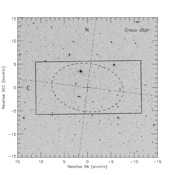
Figure 1: ESO Digital Sky Survey image centered on the Draco dSph galaxy (RA=17h 20m 12s and DEC=+57°54′55$\aas@@fstack{\prime\prime}$0). The solid line shows the observed field. The dashed ellipse shows the core radius, r_core = 7.7 arcmin and the dash-dotted lines the directions of the major and minor axes. The core radius and positions for the major and semi-major axes are taken from Irwin & Hatzidimitriou (1995).

The observations consist of one field, centered on the Draco dSph galaxy, RA=17h 20m 12s and DEC=+57°54′55$\aas@@fstack{\prime\prime}$0. Figure 1 shows the position of the field on the sky together with the core radius and position of the semi-major and semi-minor axes as given by Irwin & Hatzidimitriou (1995). The observations are summarized in Table 1.

Table 1: Summary of observations. Column 1 gives the filter; Cols. 2-6 indicate the number of 20 minute exposures in each night, Col. 7 gives the total exposure time in minutes in each filter

Filter	Night					Total
	22	23	24	25	28	Exp. time
	[min]	[min]	[min]	[min]	[min]	[min]
$y$	3$\times$20	-	1$\times$20	2$\times$20	-	120
$b$	2$\times$20	2$\times$20	2$\times$20	-	-	120
$v$	-	5$\times$20	-	1$\times$20	-	120
$u$	-	-	3$\times$20	1$\times$20	4$\times$20	160

Photometric standard stars were chosen from the list in Schuster & Nissen (1988) of secondary Strömgren standard stars. The reason for using secondary standards rather than primary Strömgren standard stars is that the latter are too bright to observe with a 2.5 m telescope. During each night approximately 15 standard stars with a large span in magnitude and colour indices, $8.137\leq y\leq 12.828,0.237\leq(b-y)\leq 0.611,0.032\leq m_{1}\leq 0.610,$ and $0.094\leq c_{1}\leq 0.490$, were observed at an airmass around 1.3. In total 43 standard stars were observed. These observations were used to obtain the colour terms in the calibration. To derive the atmospheric extinction for each night we also observed two standard stars at airmasses ranging from 1 to $\sim$2.2. These two stars will hereafter be referred to as the two extinction stars. Normally each of them was observed at six different airmasses. Table  7 lists the photometric data used in our calibration of the observed counts onto the standard system.

2.2 Photometric system

Since the standard Strömgren system for giants is based on data that does not contain any significant number of metal-poor stars (see Crawford & Barnes, 1970) all calibrations for metal-deficient stars are extrapolations from the original standard system. Although much effort is made to achieve agreement with the old standard system one should be aware that these are extrapolations and that they might differ because of differences in observational and data reduction techniques used by different authors.

The two Strömgren systems for metal-deficient giants that are commonly used are based on the catalogues by Olsen (1993) and Bond (1980). The Bond catalogue was later extended by Anthony-Twarog & Twarog (1994).

A comparison between these two systems was published by Olsen (1995), showing some systematic differences. For the $(b-y)$ and $m_{1}$ indices there is only a slight dependence on $(b-y)$ while the $c_{1}$ index shows a significant systematic difference on the order of 0.05 mag at $(b-y)$ = 0.04 and 0.02 mag at $(b-y)$ = 1.

Since we use secondary standard stars from Schuster & Nissen (1988), who used the Olsen (1993) standards to reduce their observations to the standard system, our data will be tied to the Olsen system and attention must be taken when comparing our observations with observations or models based on any other system.

Table 2: List of the photometry used for the standard stars (from Schuster & Nissen 1988). Column 1 gives the star ID; Col. 2–5 give the magnitudes and colours. The full table is available electronically.

ID	$y_{0}$	$(b-y)_{0}$	$m_{1,0}$	$c_{1,0}$
HD 33449	8.488	0.423	0.201	0.273
HD 46341	8.616	0.366	0.145	0.248
HD 51754	9.000	0.375	0.144	0.290

3 Data reduction

The entire dataset was processed using the INT Wide Field Survey pipeline provided by the Cambridge Astronomical Survey Unit (Irwin & Lewis 2001). In addition to the usual calibrations and routines that remove instrument signatures such as de-biasing, flat-fielding (using dawn and dusk sky flats obtained each night during the observing run), non-linearity, and gain corrections, the pipeline also provides tools for photometric and astrometric calibrations as well as an object catalogue. The astrometric solution is based on the Guide Star Catalog and the accuracy is $\sim$ 1″.

The object detection was done using the described pipeline. Each object that is detected is flagged as a star, an extended source, or noise. In the following we will only consider objects that were flagged as stars.

3.1 Standard star photometry and transformations

Figure 2: The residuals for the standard stars as a function of our final $(v-y)$, $\times$ (see Sect 3.1). The two extinction stars are also included (marked by an extra $\circ$). For the extinction stars we have used the mean colours and magnitudes based on all observations of these stars.

To obtain instrumental magnitudes for the standard stars we made aperture photometry, using the IRAF daophot package, on each star in a small aperture, typically around 5 pixels in radius. Using a curve-of-growth analysis we then corrected the magnitude to the radius where the curve-of-growth converged.

The transformations from the instrumental system to the standard Strömgren system were obtained by solving for the individual magnitudes rather than the colour indices. This has the advantage that we do not need to worry about the fact that observations through the different filters are, for each standard star, obtained at different airmasses (since we observe each filter separately, in contrast to four-channel photometry where observations for all four filters are obtained at the same time).

First, we derived preliminary extinction coefficients, $k_{i}$, and zero points, $z_{i}$, for each night in each filter, $i$, by solving the following set of equations using the IRAF fitparam task with a 2 $\sigma$ rejection after each fitting iteration:

$$i_{\rm s} = i_{\rm o}-k_{i}\cdot X-z_{i}$$ (1)

The standard magnitudes are on the left hand side (subscript s), instrumental magnitudes on the right hand side (subscript o), $i$ denotes any of the four filters, and $X$ is the airmass.

We then applied the preliminary $z_{i}$ and $k_{i}$ to all our standard stars from all nights and calculated preliminary colour terms, $a_{i}$,

$$i_{\rm s} = i_{\rm o}-a_{\rm i}\cdot(v-y)_{\rm s}-z_{\rm i}^{\prime}$$ (2)

where symbols are as in Eq. (1) and $a_{\rm i}$ are the colour coefficients for filter $i$. An additional zeropoint, $z_{\rm i}^{\prime}$, is introduced to improve the solution.

We then calculated a new set of $z_{i}$ and $k_{i}$ for each night using the preliminary colour terms derived above,

$$i_{\rm s} = i_{\rm o}-a_{\rm i}\cdot(v-y)_{\rm s}-k_{\rm i}\cdot X-z_{\rm i}$$ (3)

and then Eq.(2) and (3) are iterated in this way until the solutions converged. The final $z_{i}$, $k_{i}$ (for each night), and $a_{i}$ are given in Table 3.

The residuals between our photometry and the standard values are shown in Fig. 2. We note that the residuals are all small and that the scatter is $\sim$ 0.01 for $v$, $b$, and $y$ and $\sim$ 0.03 magnitudes for $u$. No offsets are found nor any residual trends with. The latter means that there is no need to add second-order terms (compare with e.g. Fig. 4 in Grundahl et al. (2002)).

Table 3: Final extinction coefficients ($k_{i}$), zero-points ($z_{i}$), and colour term coefficients, ($a_{i}$) for all filters as used in Eq. (3). Column 1 gives the dates when the observations were done; Columns 2–13 give the extinction coefficients ($k_{i}$), zero-points ($z_{i}$), and colour term coefficients, $a_{i}$ for each Strömgren filter $i$.

Night	$k_{y}$	$z_{y}$	$a_{y}$	$k_{b}$	$z_{b}$	$a_{b}$	$k_{v}$	$z_{v}$	$a_{v}$	$k_{u}$	$z_{u}$	$a_{u}$
22	0.114	–22.768	0.002	0.176	–23.207	0.020	0.275	–23.149	0.045	0.521	–23.106	0.077
23	0.124	–22.784	0.002	0.180	–23.210	0.020	0.291	–23.144	0.045	0.546	–23.103	0.077
24	0.111	–22.749	0.002	0.174	–23.191	0.020	0.284	–23.127	0.045	0.528	–23.070	0.077
25	0.117	–22.782	0.002	0.173	–23.218	0.020	0.295	–23.162	0.045	0.529	–23.092	0.077
28	0.108	–22.745	0.002	0.180	–23.201	0.020	0.284	–23.118	0.045	0.502	–22.986	0.077

3.2 Photometry for Draco

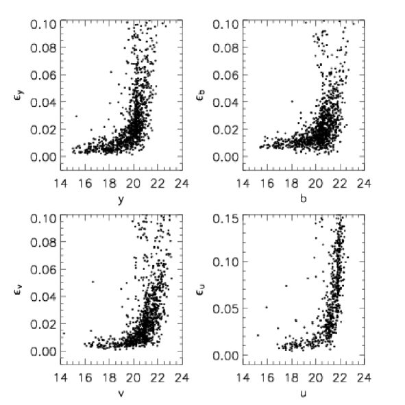
Figure 3: The resulting errors in our magnitudes for the four filters. Note the different scale on the vertical axis for $u$.

Figure 4: Errors in the $m_{\rm 1}$ and $c_{\rm 1}$ indices as a function of the $y$ magnitude.

For the science frames of the Draco dSph galaxy we again obtained aperture photometry using the daophot package in IRAF. An aperture radius of 5 pixels (1$\aas@@fstack{\prime\prime}$65) was used to minimize any effects of crowding. Using a curve of growth derived from a number of bright isolated stars on each frame we then corrected the measured magnitudes out to where the curve of growth converged. After correcting for airmass and applying zero-points for each night the photometry from the individual images were merged by averaging.

To avoid errors arising from the fact that we made our photometry on the individual frames rather than on a combined, cosmic ray cleaned frame we used the following iterative method. A mean magnitude was calculated and individual measurements falling outside $\pm 3\sigma$ of this mean were rejected. The mean was recalculated and rejections were made again. For $y$, $b$, and $v$ the second rejection was at the $\pm 1.25\sigma$-level while for $u$ we applied a second rejection level of $\pm 1.5\sigma$. The magnitudes were then converted to the standard Strömgren system using Eq. (3) with the coefficients listed in Table 3.

The photometric error for star $i$ was calculated as the error in the mean, which is defined as $\epsilon_{i}=\sigma_{i}/\sqrt{n_{i}}$, where $n_{i}$ is the number of measurements kept after the rejection process, and $\sigma_{i}$ is the standard deviation for those measurements.

The resulting errors are shown in Fig. 3. Note that the error in $u$ is larger than in the other filters since those observations are not as deep as the others. In Fig. 4 we show the resulting errors on the $m_{1}=(v-b)-(b-y)$ and $c_{1}=(u-v)-(v-b)$ Strömgren indices.

Figure 5: $y$ vs $(b-y)$ and $y$ vs $(v-y)$ colour-magnitude diagrams for the Draco dSph galaxy. $\circ$ mark all stars that were measured regardless of errors and $\bullet$ mark the stars that have $y<21$, $\epsilon_{(b-y)}<0.18$, and $\epsilon_{c_{\rm 1}}<0.18$ (see Sect. 4.1). Error bars to the right indicate typical errors in the colour at that magnitude.

3.3 Comparison with photometry from other studies

Figure 6: A comparison of our $V$ ($y_{\rm INT}$) magnitudes and $V$ magnitudes by P. Stetson ($V_{\rm Stetson}$) for stars in our field centered on the Draco dSph galaxy as a function of $y_{\rm INT}$. For stars with $15<y_{\rm INT}<17$ the offset is 0.018 magnitudes with a scatter of 0.021, while for stars with $17<y_{\rm INT}<19$ the offset is 0.007 magnitudes with a scatter of 0.021. The lower panel also includes the error-bars, which were left out from the upper panel for clarity. The broad band photometry is available at http://cadcwww.hia.nrc.ca/standards/.

Figure 7: A comparison of our $V$ ($y_{\rm INT}$) magnitudes and $V$ magnitudes by P. Stetson ($V_{\rm Stetson}$) for for stars in our field centred on the Draco dSph galaxy as a function of $(v-y)_{\rm INT}$. The broad band photometry is available at http://cadcwww.hia.nrc.ca/standards/

As an independent assessment of the quality of our data we have made a comparison between our $y$ (where we assume Strömgren $y$ = V; Olsen 1983) and the V magnitudes derived by P. Stetson. The photometric data from Stetson are available at http://cadcwww.hia.nrc.ca/standards/. Figures 6 and 7 show comparisons between our $y$ magnitudes and the Stetson $V$ magnitudes for stars in our field centred on the Draco dSph galaxy. We only make the comparison for stars that are brighter than $V=20.0$.

The differences between our and Stetson’s magnitudes appear to be an only an offset without any colour dependence. The offset is 0.018 magnitudes when the brighter stars are considered. We take this as a measure of the absolute error in the calibration of our $y$ magnitudes. That the magnitude difference decreases as the magnitudes increase reflects the fact that the two studies reach different depths with the same accuracy.

3.4 The colour-magnitude diagram

Figure 5 presents our $y$ vs $(b-y)$ and $y$ vs $(v-y)$ colour magnitude diagrams (CMD) for the stars in our field centred on the Draco dSph galaxy. The most prominent feature is the well defined RGB from $y=17$ down to $y\simeq 21.5$. A well populated horizontal branch (HB) is seen at $y\simeq 20.2$. Note the gap along the HB at $(b-y)\simeq 0.2-0.3$ and $(v-y)\simeq 0.4-0.5$ caused by the random colour and magnitude variations of the RR Lyrae stars populating this region.

A fair number of foreground objects can also be seen with $(b-y)$ in the range expected for foreground dwarf stars. These stars should mainly be situated in the thick disk and the halo of the Milky Way. The CMD shows the typical sharp cut-off at $(b-y)\simeq 0.3$ and $(v-y)\simeq 0.65$ associated with the blue limit of the turnoff stars. The various stellar populations present in the diagrams in Fig. 5 will be further discussed in Sect. 4.2.

3.5 Reddening

The reddening towards the Draco dSph galaxy is small. Stetson (1979) performed a detailed study of the reddening of stars along the line of sight towards the Draco dSph galaxy. He concluded that the total reddening (which, as the Draco dSph galaxy is essentially dust free, must emanate from the Milky Way) is $E(B-V)=0.03\pm 0.01$. We adopt this value in this paper.

The reddenings for the Strömgren indices are taken from Schlegel et al. (1998). Their scale is based on the commonly used $R_{\rm V}=3.1$ from Cardelli et al. (1989). Using the Schlegel et al. (1998) relations a reddening of $E(B-V)=0.03$ corresponds to $E(b-y)=0.023$, $E(v-y)=0.038$, $E(m_{\rm 1})=-0.008$, and $E(c_{\rm 1})=0.005$.

4 Identifying Draco members and categorising the field stars

Although the Draco dSph galaxy is at a high latitude and hence the foreground contamination is not as severe as it is in other lines of sight it is still not negligible. It is our aim to use the RGB to study the properties of the stellar populations in the Draco dSph galaxy. Therefore it is very important to confirm that the stars that appear to be on the RGB in the Draco dSph galaxy indeed are members of the dSph.

Figure 8: $c_{\rm 1,0}$ vs $(b-y)_{0}$ diagram for stars with $y<21$ and $\epsilon_{c_{\rm 1}}<0.025$. Errors as indicated. The data have been corrected for reddening according to Sect. 3.5. The standard relations for dwarf stars from Crawford (1975) and Olsen (1984) are shown with a dashed and full line, respectively. The dotted line indicates the RHB/AGB according to Anthony-Twarog & Twarog (1994) and the long-dash-short-dash and the long-dash-triple-dot lines indicate the RGB according to Anthony-Twarog & Twarog (1994) for [Fe/H] = –2 and –1.5 dex, respectively. $\circ$  denotes the stars used by Olsen (1984) to trace the MIII giants. The relations from Anthony-Twarog & Twarog (1994) have been corrected to the same system as Olsen (1993) using Olsen (1995). See also discussion in Sect. 2.2.

Figure 9: $c_{\rm 1,0}$ vs $(b-y)_{0}$ diagram for stars with $y<21$, $\epsilon_{(b-y)}<0.18$, and $\epsilon_{c_{\rm 1}}<0.18$. The data have been corrected for reddening according to Sect. 3.5. The standard relations for dwarf stars from Crawford (1975) and Olsen (1984) are shown with a dashed and full line, respectively. The dotted line indicates the RHB/AGB according to Anthony-Twarog & Twarog (1994). The relations from Anthony-Twarog & Twarog (1994) have been corrected to the same system as Olsen (1993) using Olsen (1995). See also discussion in Sect. 2.2. Large $\bullet$ indicate RGB stars, small $\bullet$  dwarf stars, $\blacktriangle$ indicates the one known carbon star inside the limits of the plot, $\times$ a small group of likely foreground dwarf stars falling below the dwarf sequence, $\oplus$ stars that cannot be easily assigned as HB or RGB stars, $\vartriangle$ stars that cannot be easily assigned as dwarf or RGB stars, open stars indicate possible AGB stars, and, finally, $+$ designate HB stars.

Figure 10: Full view of the $c_{\rm 1,0}$ vs $(b-y)_{0}$ plane for stars with $y<21$, $\epsilon_{(b-y)}<0.18$, and $\epsilon_{c_{\rm 1}}<0.18$. The data have been corrected for reddening according to Sect. 3.5. The standard relations for dwarf stars from Crawford (1975) and Olsen (1984) are shown with a full and dashed line respectively. The dotted line indicates the RHB/AGB according to Anthony-Twarog & Twarog (1994). The relations from Anthony-Twarog & Twarog (1994) have been corrected to the same system as Olsen (1993) using Olsen (1995). Stars that are neither on the dwarf or giant branches are displayed with error-bars. $\blacktriangle$ marks the known carbon stars, see Table 4, $+$ indicate probable blue HB stars or hot main sequence stars. $\circ$  denote the stars used by Olsen (1984) to trace the MIII giants.

The Strömgren photometric system gives us opportunities to identify stars at different evolutionary stages without knowing the distances to them. The $c_{\rm 1}$ index in the Strömgren system is defined to measure the Balmer discontinuity in a stellar spectrum. The blocking in the Strömgren $u$-band from metal lines is approximately twice that in the $v$-band (for a schematic diagram of this see e.g. Golay 1974, Fig. 116). Since $c_{\rm 1}=(u-v)-(v-b)$, this difference is taken care of in the construction of the index (with some remaining dependence on metallicity, see e.g. Gustafsson & Bell 1979, Fig. 23).

4.1 Selection of stars for further study

We now want to make a selection of the stars that we will base our discussions on. The three filters $v$, $b$, and $y$ all have significantly smaller errors than $u$. As we want to disentangle the different stellar populations present in the colour-magnitude diagram using the $c_{\rm 1}$ index we will be governed by the error in $u$ when selecting stars for further analysis. We later compare the results from the $c_{\rm 1}$ investigation with results from studies of radial velocity and proper motion membership. This will provide a measure of how successful our approach is and if the somewhat shallower $u$ observations are a limiting factor in our study. In Fig. 5 all stars with $y<21$, $\epsilon_{(b-y)}<0.18$, and $\epsilon_{c_{\rm 1}}<0.18$ are indicated as filled circles. These are the stars that we will consider in the following sections.

4.2 Which stellar populations do we see in the colour-magnitude diagram?

4.2.1 Finding the different populations

We start by considering the stars for which we have the very best photometry. In Fig. 8 we show the c₁ vs $(b-y)$ diagram for stars with $y<21$ and $\epsilon_{c_{\rm 1}}<0.025$.

Crawford (1975) and Olsen (1984) provide (preliminary) standard relations for field dwarf stars and a large number of stars in our data set follow these relations nicely (see Fig. 8).

The relations for RGB and red horizontal branch (RHB) and asymptotic giant branch (AGB) stars are taken from Anthony-Twarog & Twarog (1994) and have been corrected to the system of Olsen (1993) using the relations in Olsen (1995), see Sect. 2.2. We find that no star falls on the AGB sequence and that there is one probable RHB star at $(b-y)_{\rm 0}\sim 0.33$ and $c_{\rm 1,0}\sim 0.65$. A number of RGB stars fall just under the relations from Anthony-Twarog & Twarog (1994).

As giant stars with lower metallicities, at a given $(b-y)$, have higher $c_{\rm 1}$ (compare the relations shown in the figure and, more importantly, the results in Gustafsson & Bell 1979) this would indicate that the Draco dSph galaxy was significantly more metal-rich than [Fe/H]$=-1.5$. This appears unlikely as investigations of the metallicity, in a limited number of the RGB stars in the Draco dSph galaxy, have shown the metallicity of the dSph to be between $-2$ and $-1.5$ (e.g. Shetrone et al. 2001a; Bell 1985; Zinn 1978). A more likely explanation is that the empirical relations overestimate the $c_{\rm 1}$ index for RGB stars at a given metallicity.

Also shown are the stars used by Olsen (1984) to define the relation for MIII stars. As can be seen none of our stars (with very good photometry) have such red colours.

Three stars with $y<21$ and $\epsilon_{c_{\rm 1}}<0.025$ fall outside the boundaries of Fig. 8. These are (# INT, $(b-y)_{0}$, ${c_{\rm 1,0}}$, $\epsilon_{\rm(b-y)}$, $\epsilon_{c_{\rm 1}}$)= (#240, 0.328, –0.507, 0.010, 0.016), (#1961, 0.007, 1.154, 0.015, 0.020), (#1984, 0.040, 0.860, 0.012, 0.016). Stars # 1961 and 1984 fall on the continuation of the ZAMS and the HB sequence and are hence hotter foreground stars or blue HB stars. Star # 240 appears peculiar in its ${c_{\rm 1}}$, we have no simple explanation for this.

After having demonstrated how the relations in the c₁ vs $(b-y)$ plane work and where our stars with the very best photometry fall we turn to an investigation of the larger sample defined by $y<21$, $\epsilon_{(b-y)}<0.18$, and $\epsilon_{c_{\rm 1}}<0.18$ as shown in Fig. 9. This plot shows, as expected, larger scatter than Fig. 8. Nevertheless, the various standard relations are still well traced and we can easily identify the foreground dwarf stars, the RGB and RHB stars in the Draco dSph galaxy. Figure  10 is equivalent to Fig. 9 but shows the full range in ${c_{\rm 1,0}}$ and $(b-y)_{\rm 0}$ covered by our complete sample.

Foreground dwarf stars

For dwarf stars there is some metallicity dependence in the $c_{\rm 1,0}$ vs $(b-y)_{0}$ relation such that starting from around $(b-y)_{0}$ = 0.25 the less metal-rich stars fall below the solar metallicty ZAMS. This is illustrated in e.g. Fig. 13 and 14 in Clem et al. (2004). Hence we have also selected stars that fall below as well as above the relation from Olsen (1984) to be dwarf stars. Compare also our Fig. 8, 9 and 10 with Fig. 8 in Olsen (1984).

Figure 11A shows the resulting CMD for stars classified as dwarf stars.

Figure 11: $y_{0}$ vs $(b-y)_{0}$ colour-magnitude diagrams for stars with $y<21$, $\epsilon_{(b-y)}<0.18$, and $\epsilon_{(b-y)}<0.18$. A) shows stars identified as dwarf stars. B) $\triangle$ indicates stars that are not easily attributed to either the dwarf sequence or the RGB, $\times$ indicate a group of likely foreground dwarf stars,$\oplus$ stars that cannot be easily assigned as HB or RGB stars, open stars indicates possible AGB stars, and $\blacktriangle$ indicate known carbon stars (see Table 4). C) Stars identified as RGB stars. The solid lines show tracings of the RGB and HB, and are included to guide the eye.

Members of the RGB in the Draco dSph galaxy

As discussed earlier the RGB stars can be distinguished from the dwarf stars with the same colour with the help of the $c_{\rm 1}$ index. In Fig. 9 we have identified RGB stars in the Draco dSph galaxy in this way.

Around $(b-y)_{0}\sim 0.5$ there is significant uncertainty in evolutionary status for values of $c_{\rm 1,0}$ around 0.3. The same is true for stars with $(b-y)_{0}\sim 0.45$ and $c_{\rm 1,0}\sim 0.4$ where it is not clear if they belong to the RGB or HB sequence. We have handled this by collecting those stars into separate groups as indicated in Fig.  9. Figure 11B shows where these stars fall in the CMD. That our cautionary treatment of these stars is justified is exemplified by a clustering of stars around the RGB in the Draco dSph galaxy as well as a scattering towards brighter $y$ magnitudes. For the RGB stars in the Draco dSph galaxy this gives a first indication of the $(b-y)$ level at which the usage of the $c_{\rm 1}$ index as a luminosity indicator breaks down. In this case at $(b-y)_{0}$ $\sim$ 0.5 (compare Fig. 11B).

Finally, Fig. 11C shows the resulting CMD for the RGB in the Draco. One star, #2104, is far brighter than the expected RGB with $y_{0}\sim 15.9$. On closer inspection of this star’s position in the $c_{\rm 1,0}$ vs $(b-y)_{0}$ diagram we find that it is located close to the stars we that have flagged as being of uncertain status. It is thus possible that this star is a mis-classified dwarf star. Another possibility is that this star is a faint foreground giant or sub-giant star. Such stars have a typical absolute magnitude M${}_{V}\sim+2$, which means that this star would be at a vertical height of $\sim$ 3.4 kpc above the galactic plane (adopting a value of the galactic latitude in the direction of the Draco dSph galaxy, $b$ = +34.7^∘ from Mateo (1998)).

Probable AGB stars?

Based on the relation from Anthony-Twarog & Twarog (1994) we have identified four stars as probable AGB stars. However, in the CMD in Fig. 11B they do not behave like AGB stars (i.e. located along an expected AGB sequence on the blue side of the RGB).

Carbon stars

Five of the stars in the Draco dSph galaxy are known carbon stars (Table 4). Four of these stars have $y<21$, $\epsilon_{(b-y)}<0.18$, and $\epsilon_{c_{\rm 1}}<0.18$ and have been explicitly identified in Figs. 9, 10, and 11. Three of them have low $c_{\rm 1,0}$ and could therefore not be confused with the RGB stars in the $c_{\rm 1,0}$ vs $(b-y)_{0}$ diagram. We note that there are a number of stars in similar positions in the $c_{\rm 1,0}$ vs $(b-y)_{0}$ diagram and one may speculate that some of them are carbon stars. This should be further investigated using spectroscopy.

Variable stars

Our data is single-epoch and do not give any information as to the variability of the observed stars. Most of the known variables in the Draco dSph galaxy were identified by Baade & Swope (1961) using an area smaller than that covered by our images. This means that outside their image we have no knowledge about stellar variability. Our data were cross-correlated with that of Baade & Swope (1961) so that all known variables within our data were identified. None of our RGB members are known variables.

Table 4: Known carbon stars in the Draco dSph galaxy. Column 1 gives our ID; Col. 2 the name in Aaronson et al. (1982); Col. 3 the reference to each star.

INT ID	Name	Reference
1038	C4	Aaronson et al. (1982)
1119	C3	Aaronson et al. (1982)
2038	C2	Aaronson et al. (1982)
2094	C1	Aaronson et al. (1982)
2127		Shetrone et al. (2001b)

4.3 Other membership criteria

4.3.1 Radial velocities

Figure 12: $y_{0}$ vs $(b-y)_{0}$ colour-magnitude diagram for the Draco dSph galaxy and field stars cross-correlated with radial velocity studies. All stars have $y<21$, $\epsilon_{(b-y)}<0.18$, and $\epsilon_{c_{\rm 1}}<0.18$. $\bullet$ mark our RGB stars, $\circ$ mark radial velocity members from Kleyna et al. (2002) and Armandroff et al. (1995), $\square$ mark probable members from Kleyna et al., and $\times$ mark non-members from Armandroff et al. (1995) ID numbers for stars discussed in the text are included. Also shown are known carbon stars ($\triangle$). Note that the axes scales are different from previous figures. The solid lines show a fiducial of the RGB and HB to guide the eye.

Figure 13: $c_{\rm 1,0}$ vs $(b-y)_{0}$ diagrams cross-correlated with radial velocity studies. $\bullet$ mark our RGB stars, $\circ$ mark radial velocity members from Kleyna et al. (2002) and Armandroff et al. (1995), $\square$ mark probable members from Kleyna et al., and $\times$ mark non-members from Armandroff et al. ID numbers of stars discussed in the text are included. Also shown are known carbon stars ($\triangle$). The standard relations for dwarf stars from Crawford (1975) and Olsen (1984) are shown with dashed and full lines, respectively.

There are two studies in the literature with radial velocity measurements for stars in the direction of the Draco dSph galaxy: Kleyna et al. (2002) and Armandroff et al. (1995). We can utilize this information to test the procedure we used in the previous section to isolate member stars.

Since the Draco dSph galaxy (as do other dSphs) has a substantial velocity relative to the Milky Way (Mateo 1998), radial velocities of individual stars might appear as the ultimate tool to identify those that are truly members of the dSph. However, radial velocities are of limited value for (at least) two reasons: the presence of binary systems and stellar activity (Armandroff et al. 1995). Also, while radial velocity measurements can be efficiently used in the central regions of a dSph, where a large majority of the stars along the expected RGB are members, in the outer regions it is very time consuming to identify only a few real members projected onto a large amount of foreground contamination.

The most recent radial velocity study is by Kleyna et al. (2002) who list 159 members with well measured radial velocities and 27 members with less well-determined velocities. In the earlier study by Armandroff et al. (1995), an additional 91 radial velocity members are listed. Because of partial overlap in the two studies, the total number of unique radial velocity members available is 188.

Figures   12 and   13 show the CMD and $c_{\rm 1,0}$ vs $(b-y)_{0}$ diagrams for our sample of members in the Draco dSph galaxy cross-correlated with the radial velocity studies by Kleyna et al. (2002) and Armandroff et al. (1995). Out of the 188 radial velocity members 88 lie within our field and fulfill $y<21$, $\epsilon_{(b-y)}<0.18$, and $\epsilon_{c_{\rm 1}}<0.18$. All but seven of these stars were selected as RGB members when we used the $c_{\rm 1}$ index.

Four of the discrepant stars not in our RGB sample (#1038, #1119, #2094, and #2127) are known carbon stars listed in Table 6 and hence excluded from our RGB sample although they are likely members of the Draco dSph galaxy.

Star #391 falls on the RGB sequence in the CMD but is identified as a dwarf because of its position on the dwarf star sequence in the $c_{1,0}$ vs $(b-y)_{0}$ diagram (Fig. 13). However, the $c_{1}$ error for this star is large ($\epsilon_{c_{\rm 1}}\sim$ 0.36) and our classification might be erroneous.

Star #1823 is one of the stars we classify as a possible RHB/AGB star because of its location in the $c_{1,0}$ vs $(b-y)_{0}$ diagram along the RHB/RGB relation from to Anthony-Twarog & Twarog (1994) (see Fig. 9) .

The last discrepant star, #2320, is a very bright star with $y_{0}\sim 16.65$. In the CMD (Fig. 12) it falls far outside the RGB toward the blue where most of the foreground contamination is expected. In the $c_{1,0}$ vs $(b-y)_{0}$ diagram (Fig. 13) it falls on top of the dwarf star sequence and is therefore classified as a dwarf star. This star is also found in the proper motion study by Stetson (1980) which will be discussed in the next section. We note that Stetson classified this star as a non-member.

Out of the 27 stars listed as possible radial velocity members in Kleyna et al. (their Table 2), 10 stars lie within our field and 7 of those fulfill $y<21$, $\epsilon_{(b-y)}<0.18$, and $\epsilon_{c_{\rm 1}}<0.18$. Only one (# 973) is not classified as a RGB member by us. Its position in the CMD (Fig. 12) and in the $c_{1,0}$ vs $(b-y)_{0}$ diagram (Fig. 13A) shows that it is possibly a RHB/AGB star (see Schuster et al. 2004; their Fig. 6 for location of RHB/AGB stars).

Finally, we have also cross-correlated the non-Draco members listed in Armandroff et al. (1995) with our data and find that 13 stars lie within our field. 11 of those have $y<21$, $\epsilon_{(b-y)}<0.18$, and $\epsilon_{c_{\rm 1}}<0.18$. We find all of them to be foreground dwarfs stars.

That the agreement is so good between the radial velocity studies and our RGB members is not totally unexpected since Kleyna et al. (2002) especially targeted stars on the red giant branch and our $c_{\rm 1}$ selection criteria select the same type of stars. However, the result from this comparison shows that our selection method is very effective with only two cases where our classification excludes stars that are possibly members of the Draco dSph galaxy from the radial velocity studies.

4.3.2 Proper motions

Figure 14: $y_{0}$ vs $(b-y)_{0}$ colour-magnitude diagram for the Draco dSph galaxy and field stars cross-correlated with the proper motion study by Stetson (1980). All stars have $y<21$, $\epsilon_{(b-y)}<0.18$, and $\epsilon_{c_{\rm 1}}<0.18$. $\bullet$ mark our RGB stars, $\circ$ indicate stars deemed to be proper motion members based on Stetson (1980), and $\times$ indicates stars deemed to be non-members in the same study. Also shown are known carbon stars ($\triangle$). A number of stars further discussed in the text are marked by their INT numbers.

Stetson (1980) derived proper motions for a large sample of stars in the Draco dSph galaxy. The proper motions are based on measurements done on photographic plates. Based on the measured proper motion a membership probability was derived for each star. Members were then defined as stars with a probability $P>0.75$. For details of the derivation of the proper motions and probabilities the reader is referred to Stetson (1980).

In Fig.  14 we make a comparison of the selection of members of the Draco dSph galaxy based on the $c_{\rm 1}$ index and on the proper motion based probabilities. As can be seen the overall agreement is good. At the fainter end, below $y_{0}\sim$ 19.5, we find several stars that are proper motion members but not included in our member list based on the $c_{\rm 1}$ index. This is the direct result of the cuts applied in the $c_{1,0}$ vs $(b-y)_{0}$ plane as discussed in Section 4.2.1. At the brighter end the agreement is nearly perfect. A number of stars need further commenting.

There is a group of three stars at $(b-y)_{0}\sim 0.4$ and $y_{0}\sim 17.8$ which we find to be dwarfs while they are included as members in Stetson (1980). These three stars are, however, found to be non-members in Armandroff et al. (1995) in agreement with our classification.

Stars #1031 and #1046 are both identified as members using the $c_{\rm 1}$ index while considered non-members based on their proper motions. Their membership probabilities, P = 0.71 and 0.53, are, however, just below the membership cut-off, P = 0.75, used by Stetson (1980). Star #1031 is also considered as member of the Draco dSph galaxy in the radial velocity study by Armandroff et al. (1995). We therefore feel confident in including these two stars as members of the Draco dSph galaxy.

Stars #2127 and #2324 are both considered members based on their proper motions while excluded in our study. Star #2127 is, however, one of the known carbon stars listed in Table 6. Star #2324 lies clearly away from the RGB sequence and was identified as a peculiar UV-bright star in Zinn et al. (1972). Furthermore, Armandroff et al. (1995) found this star to be a non-member based on radial velocities.

4.3.3 Conclusions regarding Draco membership

Determining Draco membership through selection in the $c_{1}$ vs $(b-y)$ plane (see Sect. 4.2.1) has proven to be very accurate. We find the agreement with other studies using different methods to be very good and only a few cases are identified where the different methods disagree. Although other methods for membership determination can be efficiently used when considering the central regions of a dwarf galaxy, the $c_{1}$ index method can be used in the sparsely populated outer regions, where one would expect only a few members among a dominating foreground contamination. Table 8 shows our final list of 169 members of the Draco dSph galaxy found using the $c_{\rm 1}$ index.

The $c_{1}$ index method used here also has the advantage over other methods that it provides a way of classifying stars according to their evolutionary stage without knowing the distance to them. We refer to the excellent Figure 6 in Schuster et al. (2004) and our Figs.  9,  10, and  11 for an illustration of this.

On the other hand, we do not include stars with chemical peculiarities in our member lists since their colours may vary significantly. This is for example the case with the carbon stars listed in Table 4.

It is interesting to compare the number of “discarded” foreground stars with expectations from models of the Milky Way stellar distributions. The Besancon model of stellar population synthesis of the Milky Way (see Robin et al. 2003) predicts $\sim$ 200 foreground stars within a 0.067 square degree field (similar to ours) in the direction of the Draco dSph galaxy with $(b-y)_{0}<1.0$ and $16<y_{0}<20$. In our CMD we find a total of 213 stars not identified as RGB stars and within the magnitude and colour limits given above. This number is an upper limit since it includes known carbon stars and possibly some unidentified RGB stars on the faint end of the RGB (see Fig.  11 and discussion in Sect.  4.2.1). This number is in excellent agreement with the model prediction. This is further evidence that the method works.

Figure 15: $m_{1,0}$ vs $(b-y)_{0}$ diagram. Solid lines show isometallicity calibrations from Hilker (2000) for [Fe/H] = $-1.0$, $-1.3$, $-1.7$, and $-2.0$ dex. Dotted lines show corresponding isometallicity lines from Anthony-Twarog & Twarog (1994).

5 Metallicity in the Draco dSph galaxy

To measure the metal content of the stars we use the $m_{1}=(v-b)-(b-y)$ index. The $m_{\rm 1}$ index measures the blocking by metal lines in the $v$-band and compensates for the slope in the spectrum measured in a region where metal lines are less prominent (i.e. in the $b$ and $y$ bands). See e.g. Golay (1974) for more details on the $m_{\rm 1}$ index.

It is known that a molecular CN-band is located within the Strömgren $v$-band (e.g. Gustafsson & Bell 1979). Stars with high CN-abundances can therefore mimic stars with higher metallicities. This possibility should always be taken into account when a scatter towards high metallicities is seen in metallicity distributions based on the $m_{\rm 1}$ index. The metallicity calibrations discussed below are only valid for CN-weak/normal stars.

5.1 Metallicity calibrations

There are essentially two $m_{1}$ vs $(b-y)$ metallicity calibrations for RGB stars available in the literature. In the following section we will review and compare these calibrations in order to establish which one is the most appropriate for our data.

Figure 16: Field star giants from Clem et al. (2004) (their Table 4) selected by $log\rm{g}<3.5$ and E$(B-V)<0.03$. A) shows the difference between the tabulated metallicity and the metallicity derived using the Antony-Twarog and Twarog (1994) calibration as a function of colour. B) shows the equivalent plot using the Hilker (2000) calibration.

Antony-Twarog & Twarog (1994)

present a calibration from $m_{1}$ vs $(b-y)$ to metallicity based on a sample of metal-deficient giants. The calibration is therefore only valid in the metal-poor range $-3.2<\rm{[Fe/H]}<-1.3$ dex and within $0.4<(b-y)<0.8$.

Hilker (2000)

presents a metallicity calibration in the the $m_{1}$ vs $(b-y)$ plane for red giants valid for $-2.0<\rm{[Fe/H]}<0.0$ dex and $0.5<(b-y)<1.1$. The calibration was derived using red giants from three globular clusters ($\omega$ Centauri, M55, and M22) as well as a sample of field giants from Anthony-Twarog & Twarog (1998).

Figure 17: Field giants from Clem et al. (2004) (their Table 4) selected by $log\rm{g}<3.5$ and E$(B-V)<0.03$. Same as Fig.  16B but plotted as a function of metallicities based on spectroscopic investigations.

In Fig.  15 we compare isometallicity lines from Hilker (2000) for [Fe/H] = –1.0, –1.3, –1.7, and –2.0 dex with those of Antony-Twarog and Twarog (1994) (their Table 4) . In the region below $(b-y)_{0}$ = 0.8 the two calibrations agree reasonably well. Although the slopes are slightly different, one could expect to derive similar metallicities using either of the two calibrations in this region. A clear difference is, however, the non-linear shape of the Antony-Twarog and Twarog (1994) models above $(b-y)$ = 0.8 as compared to the Hilker (2000) calibration. The stellar sample used to derive the Antony-Twarog and Twarog (1994) calibration contained very few stars redder than $(b-y)_{0}\sim$ 0.8 and it could be an indication that the calibration is less reliable above this value.

To investigate this difference further we adopted the field star sample presented in Clem et al. (2004; their Table 4). This sample contains photometry in the four Strömgren filters as well as spectroscopic metallicities for more than 400 stars. Giants were extracted from the sample by selecting stars with $\log g<3.5$, which is the same value adopted by Clem et al. (2004), and E$(B-V)<0.03$.

By computing $\Delta[\rm{Fe/H}]$, defined as the difference between the tabulated spectroscopic metallicities and metallicities derived from the photometric calibrations, we can evaluate the two calibrations. As a first step we consider all giants within the overlapping regions of the two calibrations (i.e. $-2.0<[\rm{Fe/H}]<-1.3$ and $(b-y)>0.5$). As expected the two calibrations produce similar results for stars below $(b-y)=0.8$ (Fig. 16). Unfortunately, there is only one star in this stellar sample with $(b-y)>0.8$, i.e. where we expect the difference between the two calibrations to be significant.

Since the Hilker (2000) calibration is valid for higher metallicities, we have also included stars with $-1.0<[\rm{Fe/H}]<0.0$. A number of these stars have $(b-y)>0.8$ and Fig. 16 shows that there are no visible trends with colour. The linear approximation of the isometallicity lines in the Hilker (2000) calibration thus appear valid at the red end. The metal-poor end will be commented on further in Sec. 5.4 when the metallicities of the RGB stars in Draco dSph galaxy are discussed. We will then argue that a linear approximation is also valid at the metal-poor end.

While no trend with colour is visible in the Hilker (2000) calibration, there is a tendency for underestimating ($\Delta[\rm{Fe/H}]_{Hilker}>0$) the metallicity of stars at the metal-rich end. This is more clearly illustrated in Fig. 17, which shows the same stellar sample as in Fig. 16B but plotted against spectroscopic metallicity rather than colour. A weak trend can be seen where the metallicity of the most metal-rich stars are underestimated by, in the mean, $\sim$ 0.2 dex.

Stellar isochrones in the Strömgren system

Recently, Clem et al. (2004) derived new empirical colour-temperature relations for the Strömgren system. These were obtained by correcting stellar isochrones to fit a sample of field stars including both red giants and dwarf stars gathered from the literature (the same field star sample we adopted for the comparison above).

As noted by Clem et al. (2004), a direct comparison in the $m_{1}$ vs $(b-y)$ plane between their calibrated isochrones and the metallicity calibration by Hilker (2000) shows significant differences. In Fig.  18 we illustrate this by showing Clem et al. (2004) isochrones for [Fe/H] = –0.83, –1.54, and –2.14 dex (from their Fig. 26) overlaid on the equivalent isometallicity lines from Hilker (2000). The models agree well at the metal-poor and metal-rich end (i.e. [Fe/H] = –2.0 and 0.0 dex). There is, however, a strong discrepancy at intermediate metallicities with a difference between the two models as large as $\sim$0.5 dex at [Fe/H] $\sim$ –0.8 dex. Note that the Clem et al. (2004) isochrones fall above the equivalent Hilker (2000) isometallicity lines. This would result in an even stronger underestimate of the metallicities of the field star sample compared to the Hilker (2000) calibration. This result is surprising since the field star sample we consider is the same sample of stars used by Clem et al. (2004) to correct their models.

Figure 18: m_1,0 vs $(b-y)_{0}$ diagram. Solid lines show isometallicity calibrations from Hilker (2000) for [Fe/H] = $-0.04$, $-0.83$, $-1.54$, and $-2.14$ dex. Dashed lines show corresponding isochrones from Clem et al. (2004; their Fig. 26).

Summary

We have shown that the Hilker (2000) and Antony-Twarog and Twarog (1994) calibrations give similar results in their overlapping metallicity region and below $(b-y)=0.8$. There are no trends with colour visible in the Hilker (2000) calibration and that the linear shape of the isometallicity lines is a good approximation, at least for the metal-rich end. The Hilker (2000) calibration also has the advantage of extending up to solar metallicity and it is capable of deriving correct metallicities for an independent field star sample. We therefore adopt the Hilker (2000) calibration to derive metallicities for the RGB stars in the Draco dSph galaxy.

We note, however, that there are unexplained and significant differences between the Hilker (2000) and Clem et al. (2004) models, which should be understood before adopting these calibrations at the metal rich end. A discussion of this issue is ongoing with Clem et al. (Private communication).

5.2 Metallicity determination

Figure 19: $m_{1,0}$ vs $(b-y)_{0}$ diagram showing all our RGB stars in the Draco dSph galaxy. Overlaid are isometallicity lines from Hilker (2000) for [Fe/H] = 0.0, –1.0, –1.5, and –2.0 dex.

Figure  19 shows that the RGB members in the Draco dSph galaxy form a metal-poor population between –2.0 and –1.5 dex. For these stars we derive [Fe/H] using the calibrations from Hilker (2000). These are listed in Table 8.

Again we note that star #2104 deviates considerably from the rest of the RGB sample (compare Fig.11C). If indeed an RGB member, the metallicity for this star is close to solar, which is considerably higher than what we see for the rest of the stars in the Draco dSph galaxy. The most likely interpretation is that this star is a foreground dwarf star misidentified as RGB star (see Sect.  4.2.1).

5.3 Metallicity errors

Figure 20: Illustration of how the errors in the metallicities are derived (see Sect. 5.3). Upper panel shows the $m_{1,0}$ vs $(b-y)_{0}$ diagram with Monte Carlo simulations for three stars (#570, #1553, and #2775). Overlaid are isometallicity lines from Hilker (2000) for [Fe/H]=0.0, –1.0, –1.5, and –2.0 dex. Lower panels show corresponding metallicity distribution functions for the synthetic stars. Solid lines indicate the metallicity of the real stars. Dotted lines indicate the upper- and lower sixtile in the distribution.

To handle the error propagation from photometric errors for individual magnitudes, as shown in Fig.  3, to errors in [Fe/H] we use a Monte Carlo simulation of the data. This was done in the following way: for each magnitude of a given star (i.e. $u$, $v$, $b$, and $y$) we generate 5000 new synthetic magnitudes. These were randomly drawn from a Gaussian probability distribution with a standard deviation equal to the error ($\epsilon$) in that magnitude. New $m_{1}$ indices and $(b-y)$ colours are then calculated for each synthetic star and we derive the corresponding metallicities.

Figure  20 shows three examples of how the synthetic stars generated for star #570, #1553, and #2775 are distributed in the $m_{1,0}$ vs $(b-y)_{0}$ plane. It is interesting to note how the errors are coupled so that the synthetic stars spread out perpendicularly to the isometallicity lines. This spread is mostly driven by the error in the $b$ filter.

We also present the corresponding metallicity distribution functions for the three stars. The upper and lower sixtile of the distributions (which is equivalent to 1 $\sigma$ in the case of a Gaussian distribution) are chosen to represent our errors.

It is worth noting that the metallicity distributions for the synthetic stars are not fully symmetric. This is not surprising since the spacing of the isometallicity lines in the $m_{1,0}$ vs $(b-y)_{0}$ plane is not constant. The errors defined above are therefore not necessarily symmetric around the original [Fe/H] value. However, since the difference of the upper and lower sixtile is typically less than a few percent, we give the final [Fe/H] errors as half the distance between the upper and lower sixtile.

Figure  21 shows the final errors in [Fe/H], derived as explained above, as a function of $(b-y)_{0}$.

Figure 21: Final errors in [Fe/H] as a function of $(b-y)_{0}$ for all our RGB stars in the Draco dSph galaxy.

5.4 Comparison with spectroscopically derived metallicities

Because of the large, and to a large extent unexplained, discrepancies between the different metallicity calibrations discussed above, it is useful to compare our derived metallicities with independent measurements, e.g. spectroscopically determined metallicities. Such a comparison could also reveal any systematic shifts or trends in our data.

Abundance studies of stars in the nearby dSph galaxies are, however, difficult and time consuming due to the faintness of even the brightest of their RGB stars. In Table 5 we have collected metallicities for RGB stars in the Draco dSph galaxy available in the literature.

The most recent data set, Shetrone et al. (2001a), is based on high-resolution spectra and applies a detailed abundance analysis based on equivalent width measurements. Figure 22A shows the difference between the metallicities derived by us using the $m_{1}$ index and the values measured by Shetrone et al. (2001a) for five stars which are common to the studies. The agreement with the Shetrone et al. (2001a) values are remarkably good with a standard deviation $\sigma=0.08$ and a mean difference of 0.1 dex. In Table  5 a sixth star is included (#1701) for which Shetrone et al. (2001a) quotes [Fe/H] = –2.97 dex, or $\sim$ 0.84 dex lower than our value. The Shetrone et al. (2001a) value is well below the limit of –2.0 dex for which the Hilker (2000) metallicity calibration is valid and therefore we did not include this star in Fig. 22. In our data star #1701 falls below the –2.0 dex isometallicity line but not by much (see Fig. 19). This star is also included in the study by Zinn (1978) (see below) and the metallicity found by him is closer to the value we find than to that by Shetrone et al. (2001a).

We note that Fulbright et al. (2004) have studied this star in detail. They derive a metallicity similar to that found by Shetrone et al. (2001a) but with an effective temperature ($T_{\rm eff}$) that is $\sim 100$K larger than used in Shetrone et al. (2001a). We have calculated $T_{\rm eff}$ for all six stars in common with Shetrone et al. (2001a) using the calibrations in Alonso et al. (1999). For five of the stars (excluding #1701) the agreement between $T_{\rm eff}$ derived from $(b-y)$ and $(u-b)$ is good. For those three stars that also have $(B-V)$ from Stetson (photometry available at http://cadcwww.hia.nrc.ca/standards/) the derived $T_{\rm eff}$ also agree very well. However, all our derivations differ from the values in Shetrone et al. (2001a) such that we derive $T_{\rm eff}$ that are $\sim$100 – 200 K lower. For #1701 the agreement between $T_{\rm eff}$ derived from $(b-y)$ and $(u-b)$ is less good than for the other stars. Also, we find a temperature that is 150 K higher for $(u-b)$, in agreement with Fulbright et al. (2004). However, a change of $T_{\rm eff}$ of 150 K does not make a large enough change in [Fe/H] to explain the differences between the different studies. Neither does a change in $\log g$ (see Fulbright et al., 2004). Hence, there appears to be no easy explanation for the large discrepancy between our photometric metallicity and the metallicity derived from high resolution spectroscopy. A cautionary remark on the usage of plane parallel atmospheres in the derivation of elemental abundances for stars with $\log g<2.0$ (which is the case for the star considered here) has recently been added by Heiter & Eriksson (2006). However, to ascertain if this is the cause of the observed discrepancy needs to be further investigated by spectral modelling and is beyond the scope of this paper.

Figure 22: Comparison between our derived metallicities ([Fe/H]_m1) and values from the literature([Fe/H]_Lit): A) Shetrone et al. (2001a). B) Zinn et al. (1978) corrected to the scale by Carreta & Gratton (1997) as described in Sect.  5.4. C) Bell (1985).

The most extensive dataset is provided by Zinn (1978). His estimates of the metallicities are based on the $Q(3880)$ index (Zinn, 1978 and Zinn & Searl, 1976). Before comparing our derived metallicities to those of Zinn (1978) we apply the corrections to the Zinn & West scale described in Carretta & Gratton (1997). Figure 22B shows the comparison between our data and the corrected metallicities derived by Zinn (1978). Again, we see that our derived values are in good agreement with those of Zinn (1978). No trends can be seen and the standard deviation is $\sigma=0.13$.

Several of the stars included in the Shetrone et al. (2001a) and/or the Zinn (1978) studies have $(b-y)_{0}>0.8$ (see Table  5). Plotting the metallicity differences as a function of $(b-y)_{0}>0.8$ rather than metallicity shows that there are no trends with colour. This is encouraging since it confirms the validity of the linear shape of the Hilker (2000) metallicity lines at the metal-poor and red end, a region where the two metallicity calibrations discussed in Sec.  5.1 differed significantly.

Finally, Fig. 22C shows a comparison with abundances measured by Bell (1985). In this case we see a rather large average shift, on the order of $\sim$ 0.5 dex. Five of the stars in both Bell (1985) and our data sets are also found in either Shetrone (2001a) (three stars) and/or Zinn (1978) data (five stars). In both cases the Bell (1985) values are consistently lower by $\sim$ 0.5 dex compared to the other studies.

In conclusion, the agreement between our derived metallicities with those derived using spectroscopic methods is very good. Our errors in [Fe/H] are consistent with the spreads seen in Fig. 22A and B which show that we are not underestimating the uncertainties in our derived metallicities. The absence of large shifts between our photometric [Fe/H] and those from other studies show that our data are free from large systematic errors.

5.5 Draco metallicity distribution

Figure  23A presents the full metallicity distribution in the Draco dSph galaxy which is one of the main results of this paper. The metallicity ranges from below [Fe/H] = –2 dex to [Fe/H] $\sim$ –1.5 dex with a small tail towards higher metallicities.

Figure  23B presents the corresponding normal probability function (Devore 2000) which shows that the metallicity distribution is indeed consistent with being a single Gaussian distribution (i.e. the data points fall on a straight line). The data points only deviate significantly from a straight line at the upper right hand corner of the plot. This corresponds to the tail of metal-rich stars seen in the histogram. The solid line represents a linear least square fit to the data (excluding the outer five values at both ends) and give the mean [Fe/H] = –1.74 dex (intersection of the fitted line with x-axis = 0) and a $\sigma$ of the distribution equal to 0.24 dex (slope of the fitted line).

Figure 23: A) metallicity distribution functions for all the RGB stars in the Draco dSph galaxy (169 stars and bin size = 0.10 dex). B) shows corresponding probability plot assuming a Gaussian distribution. Solid line shows a linear fit to the data with a slope of 0.24 and the intersection with the y-axis at –1.74.

Since stars with large photometric errors (especially at the blue end) will cause large uncertainties in the derived metallicities as discussed above, we extracted a subsample of stars with errors in $\rm{[Fe/H]}$ less than 0.24 dex. Roughly half of our stars fulfill this criterion (85 out of 169). The resulting metallicity distribution and corresponding probability function for this subsample are shown in Figure 24. The derived mean [Fe/H] and $\sigma$ for this distribution (–1.75 dex and 0.25 dex, respectively) are almost identical to those of the full sample.

There is a hint of a double peak in the distribution in Fig. 23 with a main peak at [Fe/H] $\sim$ –1.8 dex and a second, smaller peak at [Fe/H] $\sim$ –1.4 dex. This secondary peak can also be seen in the full metallicity distribution in Fig.  23A . A KMM test (e.g. Ashman & Bird 1994) gives a probability of $\sim$6% that the observed distribution is drawn from a single Gaussian distribution. The corresponding probability for the subsample with low errors in their metallicities is $\sim$20%.

The corresponding probability function shows a slight “s” shape which is consistent with a bimodal distribution but this indication is weak.

We also note that the tail extending towards higher metallicities disappears when only stars with small errors are considered. This may suggest that the tail is a result of our photometric errors rather than a true intrinsic feature in the Draco dSph galaxy. A closer look at the stars constituting this metal-rich tail shows that while most of them have errors larger than the average error, they are not extreme. Many of the stars fall just outside the error cut-off for our subsample (see above and Table 8).

Figure 24: A) Metallicity distribution functions for all members of the RGB in the Draco dSph galaxy with error in $\rm{[Fe/H]}<0.24$ dex (85 stars and bin size = 0.10). Dotted line shows distribution for all members of the Draco dSph galaxy (same as in Fig.  23). B) Corresponding normal probability plot assuming a Gaussian distribution. Solid line shows a linear fit to the data with a slope of 0.25 and the intersection with the y-axis at –1.75.

It is also interesting to note that a subsample of stars which have errors in [Fe/H] that are larger than $0.4$ have distribution with an identical mean [Fe/H] = –1.74 dex and $\sigma$ = 0.24 dex as found for the full sample and also for the subsample with small errors. This indicates that it is not the errors in the derived metallicities that drive the width of the distribution but a true intrinsic metallicity spread in the Draco dSph galaxy.

The derived mean metallicity of –1.74 dex with a spread of 0.24 dex that we find for the full sample is comparable with recent studies using different methods. Lehnert et al. (1992), Dolphin (2002), Shetrone et al. (2001a), and Bellazzini et al. (2002) all find similar mean metallicities and evidence for a significant intrinsic metallicity spread comparable to ours.

Shown in Fig. 25 is a CMD of our sample of RGB stars in the Draco dSph galaxy subdivided, according to their metallicities, into three bins with $[\rm{Fe/H}]>-1.6$ dex, $-1.9<\rm{[Fe/H]}<-1.6$ dex, and $\rm{[Fe/H]}<-1.9$ dex. The metallicity bins contain 45, 77, and 47 stars, respectively. On the lower part of the RGB the metal-rich and metal-poor stars are intermingled probably as a consequence of the larger photometric errors at fainter magnitudes. Above $y\sim 18.5$, however, the metal-poor and metal-rich stars are separated in colour. The width of the RGB is well explained with a pure metallicity spread assuming an old stellar population as found by e.g. Grillmair et al (1998), Grebel (2001), and Dolphin (2002). This is illustrated in the figure by the overlaid isochrones (by Bergbusch & VandenBerg (2001) with $uvby$ colour transformations as described by Clem et al (2004)) with age = 12 Gyr and [Fe/H] = –2 and –1.5 dex. The isochrones have been shifted assuming a distance modulus of $(m-M)_{0}=19.40$ (Bonanos et al. 2004).

A similar CMD for the Carina dSph galaxy is shown in Koch et al. (2006), their Fig. 10. In that case there is no clear relation between metallicity and colour on the RGB as a result of a significant age spread. This is the well known age-metallicity degeneracy, and illustrates the importance of age-independent metallicities when deriving accurate metallicity distribution functions.

Figure 25: $y_{0}$ vs $(b-y)_{0}$ colour-magnitude diagram for all our RGB members for the Draco dSph galaxy. Large $\bullet$ indicate metal-rich stars with $\rm{[Fe/H]}>-1.6$ dex. Small $\bullet$ indicates intermediate metallicity stars with $-1.9<\rm{[Fe/H]}<-1.6$ dex. $\circ$ indicates metal-poor stars with $\rm{[Fe/H]}<-1.9$ dex. 12 Gyr isochrones by Bergbusch & VandenBerg (2001) with $uvby$ colour transformations as described by Clem et al (2004) are overlaid. The solid line indicate an isochrone with [Fe/H] = –2 dex and the dashed line with [Fe/H] = –1.5 dex.

Table 5: Abundances from the literature for stars in the Draco dSph galaxy. Columns 1 and 2 gives ID number from Baade & Swope (1961) and from this study, respectively; Col. 3-6 give our Strömgren photometry; Col. 7 the metallicity derived in this paper using the $m_{1}$ index; Col. 8-10 metallicities, effective temperatures, and $\log g$ from Shetrone et al. (2001a); Col 11 metallicities from Bell (1985) and Col. 12 metallicities from Zinn (1978).

BS	INT						S012			B85	Z78
id	id	$y_{0}$	$(b-y)_{0}$	$m_{1,0}$	$c_{1,0}$	[Fe/H]${}_{\rm m_{\rm 1}}$	[Fe/H]	Teff	$\log(g)$	[M/H]	[Fe/H]
G	1297	17.569	0.740	0.183	0.518	–2.08				–2.5	–2.02
11	1940	17.532	0.763	0.273	0.516	–1.72	–1.7	4475	0.80		–1.77
24	2082	17.073	0.856	0.243	0.585	–2.12	–2.3	4290	0.80	–2.7	–1.98
45	2097	17.621	0.733	0.201	0.535	–1.96					–1.98
49	1954	16.957	0.717	0.197	0.550	–1.93				–2.1
72	2106	18.294	0.653	0.196	0.511	–1.71					–1.81
119	1701	17.489	0.724	0.161	0.427	–2.13	–2.97	4370	0.15		–2.09
249	1988	17.216	0.885	0.423	0.457	–1.48					–1.72
267	2366	17.073	0.904	0.416	0.578	–1.56	–1.67	4180	0.60	–2.1	–1.82
286	2334	17.693	0.740	0.312	0.481	–1.45					–1.71
297	2421	17.811	0.706	0.267	0.561	–1.54					–1.88
343	1772	17.550	0.741	0.260	0.520	–1.71	–1.86	4475	0.90		–1.90
361	1112	17.424	0.793	0.365	0.498	–1.41				–2.1
473	2501	17.465	0.776	0.371	0.489	–1.32	–1.44	4400	0.90	–2.0	–1.68
506	2194	17.914	0.657	0.158	0.495	–1.94					–2.01
536	1142	16.905	0.962	0.500	0.491	–1.42				–2.3
562	1553	17.161	0.906	0.441	0.538	–1.47				–2.2	–1.74
576	1073	16.941	0.856	0.284	0.549	–1.95					–2.10
581	1110	17.627	0.762	0.321	0.525	–1.49					–1.54

5.6 Spatial metallicity distribution

It is a known fact that many dSph galaxies in the Local Group show population gradients (see e.g. Harbeck et al. 2001 and references therein; Koch et al. 2006). In the case of the Draco dSph galaxy, population gradients have been found in at least two photometric studies. Bellazini et al. (2002) find that the red HB stars are more centrally concentrated than the blue HB stars in their sample and interpret this as central concentration of more metal rich and/or younger stars. A similar trend is found by Winnick (2003). Using spectroscopic metallicities derived from the CaII triplet on a sample of 95 members of the Draco dSph galaxy, Winnick (2003) finds that the most metal-rich stars are centrally concentrated.

A conflicting result is presented by Cioni & Habing (2005), who find that if the age of the stellar population in the Draco dSph galaxy is indeed old, the metallicity increases outwards.

Since we have derived age-independent metallicities for individual stars in a clean Draco sample (i.e. we are not biased by the age-metallicity degeneracy effect), we should be able to detect spatial metallicity gradients in our data if they are present.

Figure 26 shows the spatial distribution of the RGB stars in the Draco dSph galaxy subdivided into the same three metallicity bins. The figure shows a similar trend to what is shown in Fig. 2.20 in Winnick (2003), with the metal-rich stars being more centrally concentrated than the metal poor-stars.

In Fig. 27 we show the corresponding cumulative distributions for the different metallicity bins. The fraction of stars within an ellipse with semi-major axis, a, and ellipticity = 0.33 (Irwin & Hatzidimitriou 1995) is plotted against semi-major axis, $a$. The metal-rich stars show a more centrally concentrated distribution than the metal-poor stars. A two-sided Kolmogorov-Smirnov test gives a probability of less than 2% that the metal-poor and metal-rich spatial distributions are the same. For consistency, we also include the cumulative distribution for the stars with intermediate metallicities. As expected this curve falls between the metal-rich and metal-poor distributions.

Figure 26: Spatial distribution of RGB stars in the Draco dSph galaxy. Large $\bullet$ indicate metal-rich stars with $\rm{[Fe/H]}>-1.6$ dex, small $\bullet$ stars with $-1.6<\rm{[Fe/H]}<-1.9$ dex, and $\circ$ metal-poor stars with $\rm{[Fe/H]}<-1.9$ dex. The dashed ellipse indicates the core radius from Irwin & Hatzidimitriou (1995), r${}_{core}=7.7$ arcmin.

Figure 27: Normal cumulative distribution for semimajor axis, $a$. Solid line indicates metal-rich stars with $\rm{[Fe/H]}>-1.6$ dex, dotted line stars with $-1.6<\rm{[Fe/H]}<-1.9$ dex, and dashed line metal-poor stars with $\rm{[Fe/H]}<-1.9$ dex.

6 Conclusions and summary

The aim of this study is to provide a robust method for the identification of RGB stars that are members of a dSph galaxy and determination of metallicities for individual stars along the RGB of a dSph galaxy. For the first task it is necessary to have a method that can distinguish between a foreground dwarf star and an RGB star in the dSph. The second task requires a metallicity sensitive index. The Strömgren photometric system ( $uvby$) provides both. More specifically we have:

• proven the usefulness of the Strömgren $c_{\rm 1}$ index in discriminating between RGB stars in dSph galaxies and foreground dwarf stars.
  

• presented a clean RGB sample for the Draco dSph galaxy.
  

• investigated the available metallicity calibrations for the Strömgren $m_{\rm 1}$ index
  

• derived the metallicity distribution function based on age-independent metallicities for individual stars in the inner part of the Draco dSph galaxy
  

• shown that the more metal-rich RGB stars in the Draco dSph galaxy are more centrally concentrated than the metal-poor RGB stars.
  

We also include cross correlation with the following available data sets: Stetson (1980) broad band photometry in B and V, radial velocity studies by Armandroff et al. (1995) and Kleyna et al. (2002), and Baade & Swope (1961) list of variable stars in the Draco dSph galaxy.

Membership has been determined using the Strömgren $c_{\rm 1}$-colour index. Comparison with alternative methods of membership determination (e.g. proper motion and radial velocity measurements) show that our membership classification agrees very well with other methods. We are therefore confident that the same method for membership determination, i.e. selection in the $c_{\rm 1}$ vs $(b-y)$-plane, can now be applied to the sparsely populated outer regions of dSphs.

In addition to the ability to identify dSph members using the $c_{\rm 1}$ index, the Strömgren system provides the possibility to derive individual and age-independent metallicities for RGB stars using the $m_{\rm 1}$ index. Since our metallicity determination is age independent, our results are not limited by the age-metallicity degeneracy (which is the case for most other photometric metallicity studies).

A review of the existing Strömgren metallicity calibrations for giant stars has led us to use the calibration by Hilker (2000). Applying it to our clean sample of members of the Draco dSph galaxy we present individual metallicities for 169 stars, the largest independent sample so far for the Draco dSph galaxy. The photometrically derived metallicities agree very well with high-resolution spectroscopic determinations (i.e. Shetrone et al., 2001a) and with earlier results from spectral indices (Zinn, 1978).

The metallicity distribution function we obtain is consistent with a single Gaussian distribution with a mean metallicity [Fe/H] = –1.74 dex and a $\sigma$ = 0.25 dex and with a small tail of more metal-rich stars.

Although the data presented in this paper only include the central regions of the Draco dSph galaxy, we have investigated the spatial metallicity distribution and find evidence for a central concentration of more metal-rich stars.

Table 6: RGB stars in the Draco dSph galaxy. Column 1 gives the ID number from this study; Col. 2 gives the designation from Stetson’s photometric catalog (available at http://cadcwww.hia.nrc.ca/standards/); Cols. 3 and 4 give the pixel position on the CCD; Cols. 5 and 6 give the position on the sky, Cols. 7 – 10 give our Strömgren photometry and Col. 11 the metallicity derived in this paper using the $m_{1}$ index. Column 12 gives the membership probability based on proper motions given in Stetson (1980). Finally Col. 13 gives radial velocities from Kleyna et al. (2002).

INT ID	Other ID	x	y	R.A. (2000)	Dec (2000)	$y\pm\epsilon_{y}$	$b\pm\epsilon_{b}$	$v\pm\epsilon_{v}$	$u\pm\epsilon_{u}$	[Fe/H]${}_{\rm m_{\rm 1}}$	P	$V_{\rm r}$
53		676.192	69.349	4.5446477	1.0113240	19.801 $\pm$ 0.022	20.347 $\pm$ 0.014	20.854 $\pm$ 0.049	21.706 $\pm$ 0.171	-2.79$\pm$0.20
92	S-366	1838.474	125.208	4.5444217	1.0094626	17.423 $\pm$ 0.018	18.188 $\pm$ 0.023	19.146 $\pm$ 0.012	20.559 $\pm$ 0.079	-2.09$\pm$0.14		-304.75
162		909.711	228.023	4.5441618	1.0109553	19.260 $\pm$ 0.041	19.758 $\pm$ 0.029	20.297 $\pm$ 0.032	21.225 $\pm$ 0.106	-2.03$\pm$0.37

Table 7: List of standard stars used (from Schuster & Nissen 1988). Column 1 gives the star ID; Col. 2–5 give the magnitudes and colours.

ID	$y_{0}$	$(b-y)_{0}$	$m_{1,0}$	$c_{1,0}$
HD 33449	8.488	0.423	0.201	0.273
HD 46341	8.616	0.366	0.145	0.248
HD 51754	9.000	0.375	0.144	0.290
HD 64090	8.279	0.428	0.110	0.126
HD 75530	9.167	0.443	0.254	0.257
HD 81408	9.610	0.560	0.478	0.210
HD 88371	8.414	0.407	0.186	0.329
HD 107853	9.081	0.317	0.157	0.483
HD 107583	9.33	0.375	0.183	0.319
HD 108754	9.006	0.435	0.217	0.254
HD 118659	8.827	0.422	0.196	0.244
HD 123265	8.348	0.504	0.356	0.348
HD 131653	9.506	0.442	0.226	0.253
HD 132475	8.555	0.401	0.063	0.285
HD 134088	7.992	0.392	0.137	0.255
HD 134439	9.058	0.484	0.224	0.165
HD 134440	9.419	0.524	0.297	0.173
HD 137303	8.774	0.611	0.610	0.178
HD 138648	8.137	0.504	0.358	0.290
HD 149414	9.611	0.476	0.202	0.162
HD 161770	9.696	0.489	0.036	0.301
HD 163810	9.635	0.423	0.114	0.199
HD 175179	9.072	0.384	0.146	0.268
HD 175617	10.130	0.441	0.208	0.281
HD 220769	9.31	0.340	0.140	0.310
G 9 -031	10.823	0.398	0.158	0.224
G 9 -036	11.934	0.381	0.124	0.195
G 14 -024	12.822	0.509	0.123	0.094
G 14 -039	12.828	0.587	0.267	0.153
G 14 -045	10.803	0.587	0.517	0.115
G 63 -026	12.183	0.328	0.085	0.277
DM -14 4454	10.332	0.565	0.469	0.192
DM -14 3322	10.394	0.377	0.131	0.220
DM -13 2948	9.439	0.426	0.256	0.221
DM -13 3834	10.685	0.415	0.098	0.183
DM -12 2669	10.230	0.229	0.094	0.490
DM -9 3102	10.479	0.425	0.202	0.206
DM -8 4501	10.591	0.452	0.032	0.274
DM -5 3063	9.734	0.568	0.461	0.182
DM -5 2678	10.654	0.296	0.155	0.422
DM -5 3763	10.239	0.579	0.546	0.241
DM -4 3208	9.998	0.311	0.048	0.373
DM +25 1981	9.317	0.237	0.103	0.489

Table 8: Draco RGB stars. Column 1 gives the ID number from this study; Col. 2 gives the designation from Stetson’s photometric catalog (available at http://cadcwww.hia.nrc.ca/standards/); Cols. 3 and 4 give the pixel position on the CCD; Cols. 5 and 6 give the position on the sky, Cols. 7 – 10 give our Strömgren photometry and Col. 11 the metallicity derived in this paper using the $m_{1}$ index. Column 12 gives the membership probability based on proper motions given in Stetson (1980). Finally Col. 13 gives radial velocities from Kleyna et al. (2002).

INT ID	Other ID	x	y	R.A. (2000)	Dec (2000)	$y\pm\epsilon_{y}$	$b\pm\epsilon_{b}$	$v\pm\epsilon_{v}$	$u\pm\epsilon_{u}$	[Fe/H]${}_{\rm m_{\rm 1}}$	P	$V_{\rm r}$
53		676.192	69.349	4.5446477	1.0113240	19.801 $\pm$ 0.022	20.347 $\pm$ 0.014	20.854 $\pm$ 0.049	21.706 $\pm$ 0.171	-2.79$\pm$0.20
92	S-366	1838.474	125.208	4.5444217	1.0094626	17.423 $\pm$ 0.018	18.188 $\pm$ 0.023	19.146 $\pm$ 0.012	20.559 $\pm$ 0.079	-2.09$\pm$0.14
162		909.711	228.023	4.5441618	1.0109553	19.260 $\pm$ 0.041	19.758 $\pm$ 0.029	20.297 $\pm$ 0.032	21.225 $\pm$ 0.106	-2.03$\pm$0.37
167		404.888	231.823	4.5441723	1.0117639	19.127 $\pm$ 0.044	19.656 $\pm$ 0.035	20.253 $\pm$ 0.017	21.254 $\pm$ 0.124	-1.99$\pm$0.38
243	S-348	1698.858	324.059	4.5438347	1.0096923	19.585 $\pm$ 0.050	20.118 $\pm$ 0.043	20.726 $\pm$ 0.026	21.692 $\pm$ 0.241	-1.94$\pm$0.47
266	S-346	1420.164	360.157	4.5437412	1.0101408	19.027 $\pm$ 0.032	19.548 $\pm$ 0.033	20.128 $\pm$ 0.014	21.131 $\pm$ 0.056	-2.02$\pm$0.33
338		741.701	444.257	4.5435209	1.0112317	18.450 $\pm$ 0.019	19.058 $\pm$ 0.043	19.833 $\pm$ 0.036	20.979 $\pm$ 0.400	-1.69$\pm$0.35		-291.42
372		539.093	506.334	4.5433431	1.0115584	18.231 $\pm$ 0.026	18.817 $\pm$ 0.033	19.520 $\pm$ 0.014	20.630 $\pm$ 0.084	-1.90$\pm$0.29
374	S-338	1135.257	519.022	4.5432787	1.0106027	18.828 $\pm$ 0.022	19.401 $\pm$ 0.024	20.094 $\pm$ 0.032	21.167 $\pm$ 0.088	-1.82$\pm$0.24
378		1500.894	509.574	4.5432892	1.0100154	17.964 $\pm$ 0.087	18.642 $\pm$ 0.072	19.532 $\pm$ 0.026	20.758 $\pm$ 0.097	-1.72$\pm$0.62
379	S-337	1465.066	521.863	4.5432544	1.0100733	18.165 $\pm$ 0.018	18.776 $\pm$ 0.022	19.566 $\pm$ 0.009	20.718 $\pm$ 0.126	-1.63$\pm$0.18
570		606.555	793.316	4.5424771	1.0114594	17.261 $\pm$ 0.017	18.048 $\pm$ 0.030	19.072 $\pm$ 0.011	20.629 $\pm$ 0.038	-1.96$\pm$0.18
571	S-311	814.854	798.362	4.5424533	1.0111253	18.210 $\pm$ 0.027	18.862 $\pm$ 0.032	19.725 $\pm$ 0.017	20.979 $\pm$ 0.128	-1.62$\pm$0.25
574		1898.897	789.996	4.5424275	1.0093836	18.885 $\pm$ 0.016	19.465 $\pm$ 0.023	20.115 $\pm$ 0.016	21.100 $\pm$ 0.083	-2.17$\pm$0.19
576		1402.435	803.061	4.5424128	1.0101818	19.057 $\pm$ 0.023	19.604 $\pm$ 0.027	20.277 $\pm$ 0.029	21.281 $\pm$ 0.217	-1.67$\pm$0.28
593	S-302	2016.722	842.690	4.5422630	1.0091954	18.521 $\pm$ 0.011	19.131 $\pm$ 0.019	19.867 $\pm$ 0.023	20.964 $\pm$ 0.128	-1.94$\pm$0.15
639		1799.953	932.962	4.5420027	1.0095463	19.564 $\pm$ 0.022	20.089 $\pm$ 0.041	20.701 $\pm$ 0.038	21.668 $\pm$ 0.257	-1.83$\pm$0.40
649	S-301	1402.435	803.061	4.5424128	1.0101818	19.057 $\pm$ 0.023	19.604 $\pm$ 0.027	20.277 $\pm$ 0.029	21.281 $\pm$ 0.217	-1.67$\pm$0.28
593		1547.761	945.233	4.5419779	1.0099521	18.528 $\pm$ 0.003	19.118 $\pm$ 0.031	19.831 $\pm$ 0.010	20.948 $\pm$ 0.046	-1.88$\pm$0.23
729	S-298	1057.142	1023.448	4.5417652	1.0107428	17.776 $\pm$ 0.018	18.473 $\pm$ 0.026	19.365 $\pm$ 0.016	20.715 $\pm$ 0.048	-1.88$\pm$0.18
752		733.721	1046.272	4.5417094	1.0112629	18.911 $\pm$ 0.024	19.453 $\pm$ 0.029	20.096 $\pm$ 0.011	21.122 $\pm$ 0.086	-1.80$\pm$0.27	0.94
760		416.900	1032.803	4.5417633	1.0117707	17.975 $\pm$ 0.013	18.667 $\pm$ 0.007	19.585 $\pm$ 0.048	20.942 $\pm$ 0.091	-1.71$\pm$0.13
798		129.392	1076.583	4.5416422	1.0122328	17.449 $\pm$ 0.028	18.232 $\pm$ 0.036	19.346 $\pm$ 0.017	20.951 $\pm$ 0.067	-1.52$\pm$0.22
800	S-293	1693.595	1081.475	4.5415611	1.0097210	17.824 $\pm$ 0.014	18.481 $\pm$ 0.026	19.271 $\pm$ 0.008	20.495 $\pm$ 0.056	-2.08$\pm$0.19
810		400.710	1086.382	4.5416021	1.0117984	18.888 $\pm$ 0.014	19.442 $\pm$ 0.030	20.083 $\pm$ 0.026	21.063 $\pm$ 0.111	-1.96$\pm$0.27
864		1156.473	1170.984	4.5413156	1.0105871	18.910 $\pm$ 0.009	19.454 $\pm$ 0.020	20.131 $\pm$ 0.020	21.135 $\pm$ 0.090	-1.61$\pm$0.19	0.93
877		107.980	1179.928	4.5413308	1.0122702	17.297 $\pm$ 0.025	18.099 $\pm$ 0.034	19.270 $\pm$ 0.008	20.942 $\pm$ 0.142	-1.42$\pm$0.22
884	S-286	1443.377	1192.707	4.5412374	1.0101264	19.260 $\pm$ 0.023	19.754 $\pm$ 0.032	20.312 $\pm$ 0.033	21.233 $\pm$ 0.116	-1.84$\pm$0.37
902	S-285	1469.530	1214.630	4.5411701	1.0100847	19.469 $\pm$ 0.028	20.019 $\pm$ 0.032	20.640 $\pm$ 0.018	21.577 $\pm$ 0.287	-2.05$\pm$0.30
907	392	877.310	1217.484	4.5411873	1.0110371	18.532 $\pm$ 0.017	19.155 $\pm$ 0.033	19.973 $\pm$ 0.011	21.121 $\pm$ 0.179	-1.59$\pm$0.26	0.85
910	386	1002.836	1242.023	4.5411077	1.0108360	19.121 $\pm$ 0.035	19.704 $\pm$ 0.025	20.444 $\pm$ 0.051	21.506 $\pm$ 0.141	-1.65$\pm$0.31
922	S-283	1605.947	1236.966	4.5410967	1.0098660	18.791 $\pm$ 0.035	19.361 $\pm$ 0.009	20.037 $\pm$ 0.019	21.083 $\pm$ 0.109	-1.91$\pm$0.19
939		1777.872	1262.273	4.5410123	1.0095899	18.736 $\pm$ 0.037	19.310 $\pm$ 0.031	20.011 $\pm$ 0.025	21.133 $\pm$ 0.085	-1.78$\pm$0.31
956		1998.828	1290.207	4.5409174	1.0092350	19.092 $\pm$ 0.010	19.644 $\pm$ 0.019	20.284 $\pm$ 0.028	21.360 $\pm$ 0.164	-1.95$\pm$0.18
980		22.130	1324.380	4.5408974	1.0124120	16.809 $\pm$ 0.014	17.699 $\pm$ 0.028	18.929 $\pm$ 0.072	20.750 $\pm$ 0.147	-1.82$\pm$0.19
993		768.016	1350.871	4.5407887	1.0112163	18.542 $\pm$ 0.024	19.147 $\pm$ 0.020	19.909 $\pm$ 0.022	21.063 $\pm$ 0.094	-1.74$\pm$0.20	0.95
996	S-274	1680.806	1349.157	4.5407548	1.0097482	18.119 $\pm$ 0.005	18.777 $\pm$ 0.023	19.626 $\pm$ 0.008	20.936 $\pm$ 0.094	-1.76$\pm$0.15
1006	S-273	1756.981	1351.336	4.5407443	1.0096257	18.572 $\pm$ 0.022	19.147 $\pm$ 0.019	19.823 $\pm$ 0.016	20.861 $\pm$ 0.155	-1.97$\pm$0.18
1024	544	1441.549	1367.591	4.5407100	1.0101336	18.926 $\pm$ 0.041	19.496 $\pm$ 0.020	20.201 $\pm$ 0.023	21.314 $\pm$ 0.228	-1.72$\pm$0.28	0.88
1031	414	542.374	1355.997	4.5407825	1.0115788	16.428 $\pm$ 0.044	17.366 $\pm$ 0.038	18.777 $\pm$ 0.009	20.673 $\pm$ 0.100	-1.45$\pm$0.21	0.71	-300.47

Table 8: Continued.

INT ID	Other ID	x	y	R.A. (2000)	Dec (2000)	$y\pm\epsilon_{y}$	$b\pm\epsilon_{b}$	$v\pm\epsilon_{v}$	$u\pm\epsilon_{u}$	[Fe/H]${}_{\rm m_{\rm 1}}$	P	$V_{\rm r}$
1032		561.460	1379.797	4.5407100	1.0115488	18.692 $\pm$ 0.118	19.261 $\pm$ 0.020	20.039 $\pm$ 0.085	21.222 $\pm$ 0.307	-1.23$\pm$0.74
1041		24.222	1403.295	4.5406590	1.0124109	19.176 $\pm$ 0.042	19.709 $\pm$ 0.034	20.346 $\pm$ 0.043	21.376 $\pm$ 0.065	-1.75$\pm$0.41
1046	542	1497.098	1403.805	4.5405979	1.0100452	19.377 $\pm$ 0.031	19.926 $\pm$ 0.049	20.575 $\pm$ 0.044	21.569 $\pm$ 0.125	-1.85$\pm$0.45	0.53
1051		658.005	1404.104	4.5406322	1.0113945	19.004 $\pm$ 0.044	19.512 $\pm$ 0.045	20.101 $\pm$ 0.014	21.083 $\pm$ 0.202	-1.78$\pm$0.50	0.97
1072		268.593	1415.126	4.5406141	1.0120198	18.495 $\pm$ 0.031	19.095 $\pm$ 0.042	19.847 $\pm$ 0.035	21.003 $\pm$ 0.122	-1.74$\pm$0.38
1073	576	242.520	1427.791	4.5405765	1.0120618	16.941 $\pm$ 0.017	17.797 $\pm$ 0.023	18.937 $\pm$ 0.030	20.626 $\pm$ 0.086	-1.95$\pm$0.13		-282.44
1079	166	887.666	1445.687	4.5404973	1.0110265	19.169 $\pm$ 0.036	19.684 $\pm$ 0.042	20.329 $\pm$ 0.025	21.347 $\pm$ 0.134	-1.46$\pm$0.47	0.97
1084	377	1088.096	1454.157	4.5404639	1.0107045	18.718 $\pm$ 0.025	19.226 $\pm$ 0.019	19.843 $\pm$ 0.011	20.829 $\pm$ 0.113	-1.59$\pm$0.23	0.94
1101	372	1195.812	1495.384	4.5403342	1.0105323	19.661 $\pm$ 0.074	20.175 $\pm$ 0.041	20.814 $\pm$ 0.032	21.793 $\pm$ 0.231	-1.48$\pm$0.64	0.31
1104		424.930	1493.678	4.5403705	1.0117711	18.736 $\pm$ 0.038	19.245 $\pm$ 0.021	19.874 $\pm$ 0.018	20.885 $\pm$ 0.081	-1.50$\pm$0.31	0.97
1110	581	109.851	1492.713	4.5403848	1.0122763	17.627 $\pm$ 0.028	18.389 $\pm$ 0.040	19.472 $\pm$ 0.023	21.080 $\pm$ 0.111	-1.49$\pm$0.26	0.83	-301.95
1112	361	1271.348	1491.454	4.5403433	1.0104107	17.424 $\pm$ 0.008	18.217 $\pm$ 0.027	19.376 $\pm$ 0.019	21.033 $\pm$ 0.093	-1.41$\pm$0.15	0.95	-287.25
1142	536	1596.831	1519.234	4.5402455	1.0098875	16.905 $\pm$ 0.012	17.867 $\pm$ 0.016	19.328 $\pm$ 0.015	21.280 $\pm$ 0.181	-1.42$\pm$0.08	0.94	-300.67
1159		1744.505	1545.400	4.5401597	1.0096503	18.178 $\pm$ 0.014	18.811 $\pm$ 0.023	19.650 $\pm$ 0.015	20.912 $\pm$ 0.095	-1.58$\pm$0.18
1191		997.708	1583.382	4.5400767	1.0108532	19.094 $\pm$ 0.031	19.636 $\pm$ 0.026	20.378 $\pm$ 0.034	21.471 $\pm$ 0.193	-1.13$\pm$0.32	0.96
1202	427	447.718	1574.937	4.5401239	1.0117366	18.082 $\pm$ 0.009	18.729 $\pm$ 0.045	19.620 $\pm$ 0.015	20.924 $\pm$ 0.049	-1.42$\pm$0.32	0.97	-301.76
1223	153	1269.643	1620.402	4.5399537	1.0104165	18.490 $\pm$ 0.014	19.066 $\pm$ 0.018	19.869 $\pm$ 0.009	21.075 $\pm$ 0.052	-1.15$\pm$0.17	0.97
1297	G	669.692	1663.150	4.5398479	1.0113825	17.569 $\pm$ 0.011	18.309 $\pm$ 0.025	19.232 $\pm$ 0.016	20.673 $\pm$ 0.054	-2.08$\pm$0.15	0.97
1324	194	791.767	1664.778	4.5398383	1.0111864	18.262 $\pm$ 0.024	18.897 $\pm$ 0.027	19.746 $\pm$ 0.012	21.059 $\pm$ 0.105	-1.53$\pm$0.23	0.97
1341	146	1037.402	1716.289	4.5396729	1.0107925	18.567 $\pm$ 0.019	19.179 $\pm$ 0.038	19.935 $\pm$ 0.019	21.056 $\pm$ 0.156	-1.84$\pm$0.30	0.96
1356	219	623.093	1732.477	4.5396404	1.0114591	18.470 $\pm$ 0.032	19.104 $\pm$ 0.030	19.892 $\pm$ 0.013	21.183 $\pm$ 0.164	-1.86$\pm$0.25	0.96
1359	171	964.446	1725.615	4.5396476	1.0109102	18.861 $\pm$ 0.044	19.458 $\pm$ 0.019	20.220 $\pm$ 0.029	21.329 $\pm$ 0.166	-1.65$\pm$0.26	0.94
1360	172	963.479	1737.057	4.5396132	1.0109119	18.895 $\pm$ 0.103	19.488 $\pm$ 0.040	20.196 $\pm$ 0.054	21.309 $\pm$ 0.225	-1.95$\pm$0.61	0.94
1365	195	751.090	1738.848	4.5396156	1.0112535	18.579 $\pm$ 0.017	19.169 $\pm$ 0.031	19.886 $\pm$ 0.021	20.995 $\pm$ 0.065	-1.86$\pm$0.25	0.97
1444		2012.633	1795.190	4.5393939	1.0092242	17.529 $\pm$ 0.013	18.274 $\pm$ 0.006	19.321 $\pm$ 0.007	20.798 $\pm$ 0.062	-1.51$\pm$0.06
1458	350	1558.326	1819.533	4.5393395	1.0099564	18.189 $\pm$ 0.012	18.817 $\pm$ 0.036	19.602 $\pm$ 0.013	20.837 $\pm$ 0.137	-1.83$\pm$0.26	0.94	-289.00
1553	562	824.661	1044.222	4.5417123	1.0111169	17.161 $\pm$ 0.017	18.066 $\pm$ 0.024	19.413 $\pm$ 0.016	21.298 $\pm$ 0.169	-1.47$\pm$0.12	0.97	-295.02
1567	558	1010.729	1159.957	4.5413556	1.0108211	18.566 $\pm$ 0.022	19.158 $\pm$ 0.021	19.864 $\pm$ 0.016	20.964 $\pm$ 0.087	-1.95$\pm$0.19	0.91
1647	122	1336.791	1904.973	4.5390902	1.0103151	17.969 $\pm$ 0.016	18.646 $\pm$ 0.063	19.654 $\pm$ 0.017	21.016 $\pm$ 0.136	-1.09$\pm$0.45
1654	L	794.353	1910.505	4.5390944	1.0111881	18.168 $\pm$ 0.038	18.831 $\pm$ 0.035	19.681 $\pm$ 0.010	21.044 $\pm$ 0.052	-1.79$\pm$0.28	0.97
1701	119	1385.871	1923.999	4.5390306	1.0102365	17.489 $\pm$ 0.009	18.213 $\pm$ 0.010	19.098 $\pm$ 0.021	20.411 $\pm$ 0.065	-2.13$\pm$0.08	0.92	-295.13
1707	H	1243.583	1935.957	4.5390000	1.0104659	18.120 $\pm$ 0.012	18.728 $\pm$ 0.016	19.465 $\pm$ 0.016	20.668 $\pm$ 0.069	-1.92$\pm$0.13	0.97
1738	N	755.207	1964.317	4.5389328	1.0112524	18.922 $\pm$ 0.029	19.490 $\pm$ 0.043	20.148 $\pm$ 0.019	21.201 $\pm$ 0.259	-1.99$\pm$0.39	0.97
1744	99	1238.353	1978.347	4.5388718	1.0104752	19.703 $\pm$ 0.053	20.245 $\pm$ 0.030	20.849 $\pm$ 0.089	21.904 $\pm$ 0.299	-2.08$\pm$0.46	0.97
1746	131	1118.448	1977.566	4.5388784	1.0106683	19.244 $\pm$ 0.024	19.737 $\pm$ 0.033	20.324 $\pm$ 0.038	21.283 $\pm$ 0.078	-1.60$\pm$0.37	0.97
1766	340	1496.295	1993.884	4.5388141	1.0100602	19.384 $\pm$ 0.028	19.904 $\pm$ 0.032	20.597 $\pm$ 0.018	21.629 $\pm$ 0.251	-1.17$\pm$0.35	0.97
1770	97	1184.827	2003.372	4.5387983	1.0105619	19.366 $\pm$ 0.074	19.896 $\pm$ 0.040	20.566 $\pm$ 0.024	21.609 $\pm$ 0.112	-1.48$\pm$0.58	0.95
1772	343	1557.547	1984.207	4.5388412	1.0099612	17.550 $\pm$ 0.003	18.291 $\pm$ 0.029	19.291 $\pm$ 0.010	20.812 $\pm$ 0.049	-1.71$\pm$0.17	0.91	-293.96
1787	116	1371.305	2021.150	4.5387368	1.0102620	19.128 $\pm$ 0.037	19.715 $\pm$ 0.031	20.466 $\pm$ 0.024	21.538 $\pm$ 0.202	-1.61$\pm$0.30	0.97
1788	115	1348.013	2024.958	4.5387263	1.0102997	19.183 $\pm$ 0.018	19.699 $\pm$ 0.031	20.334 $\pm$ 0.022	21.410 $\pm$ 0.072	-1.54$\pm$0.33	0.93
1790		1987.967	2023.971	4.5387034	1.0092688	18.045 $\pm$ 0.007	18.710 $\pm$ 0.015	19.573 $\pm$ 0.013	20.840 $\pm$ 0.079	-1.75$\pm$0.11
1791	Q	745.022	2031.946	4.5387282	1.0112703	19.553 $\pm$ 0.051	20.078 $\pm$ 0.040	20.650 $\pm$ 0.027	21.647 $\pm$ 0.206	-2.11$\pm$0.45	0.89
1807	O	695.720	2055.535	4.5386586	1.0113502	19.059 $\pm$ 0.038	19.662 $\pm$ 0.044	20.359 $\pm$ 0.014	21.486 $\pm$ 0.174	-2.10$\pm$0.36	0.94

Table 8: Continued.

INT ID	Other ID	x	y	R.A. (2000)	Dec (2000)	$y\pm\epsilon_{y}$	$b\pm\epsilon_{b}$	$v\pm\epsilon_{v}$	$u\pm\epsilon_{u}$	[Fe/H]${}_{\rm m_{\rm 1}}$	P	$V_{\rm r}$
1813	114	1338.130	2062.865	4.5386119	1.0103164	18.714 $\pm$ 0.019	19.305 $\pm$ 0.031	20.055 $\pm$ 0.019	21.215 $\pm$ 0.064	-1.66$\pm$0.25	0.94
1843	437	282.485	1916.420	4.5390954	1.0120106	17.640 $\pm$ 0.010	18.392 $\pm$ 0.016	19.395 $\pm$ 0.023	20.801 $\pm$ 0.122	-1.79$\pm$0.11	0.97	-307.83
1849		370.640	2096.281	4.5385470	1.0118735	19.613 $\pm$ 0.089	20.149 $\pm$ 0.041	20.795 $\pm$ 0.066	21.835 $\pm$ 0.314	-1.72$\pm$0.67	0.97
1893	335	1445.807	2144.639	4.5383596	1.0101447	18.062 $\pm$ 0.009	18.726 $\pm$ 0.024	19.639 $\pm$ 0.014	21.010 $\pm$ 0.039	-1.45$\pm$0.17	0.96	-288.59
1900		2027.494	2154.508	4.5383072	1.0092077	19.128 $\pm$ 0.018	19.642 $\pm$ 0.015	20.246 $\pm$ 0.039	21.218 $\pm$ 0.039	-1.76$\pm$0.22
1911	55	858.762	2156.976	4.5383449	1.0110902	19.320 $\pm$ 0.019	19.848 $\pm$ 0.019	20.391 $\pm$ 0.029	21.335 $\pm$ 0.158	-2.36$\pm$0.20	0.96
1925	M	1097.671	2136.035	4.5383992	1.0107052	18.688 $\pm$ 0.028	19.287 $\pm$ 0.027	20.050 $\pm$ 0.027	21.194 $\pm$ 0.076	-1.66$\pm$0.25	0.95
1929	108	1366.025	2175.235	4.5382705	1.0102739	19.241 $\pm$ 0.020	19.791 $\pm$ 0.036	20.506 $\pm$ 0.048	21.584 $\pm$ 0.110	-1.42$\pm$0.34	0.90
1933		1864.355	2176.953	4.5382457	1.0094711	18.083 $\pm$ 0.009	18.732 $\pm$ 0.018	19.546 $\pm$ 0.013	20.832 $\pm$ 0.063	-1.87$\pm$0.13
1940	11	495.329	2186.303	4.5382695	1.0116751	17.532 $\pm$ 0.030	18.295 $\pm$ 0.020	19.331 $\pm$ 0.018	20.883 $\pm$ 0.052	-1.72$\pm$0.16	0.97	-283.92
1954	49	764.593	2180.260	4.5382776	1.0112422	16.957 $\pm$ 0.019	17.674 $\pm$ 0.026	18.588 $\pm$ 0.012	20.052 $\pm$ 0.083	-1.93$\pm$0.17	0.97	-289.39
1988	249	267.862	2229.794	4.5381455	1.0120414	17.216 $\pm$ 0.005	18.101 $\pm$ 0.026	19.410 $\pm$ 0.023	21.175 $\pm$ 0.138	-1.48$\pm$0.13	0.76	-293.11
2014	22	641.982	2282.425	4.5379725	1.0114416	18.086 $\pm$ 0.021	18.778 $\pm$ 0.012	19.674 $\pm$ 0.020	21.059 $\pm$ 0.067	-1.81$\pm$0.12	0.92	-298.52
2026	322	1388.866	2298.269	4.5378971	1.0102396	18.813 $\pm$ 0.007	19.407 $\pm$ 0.031	20.157 $\pm$ 0.027	21.355 $\pm$ 0.086	-1.68$\pm$0.24	0.92
2027	33	519.499	2298.652	4.5379281	1.0116388	18.681 $\pm$ 0.024	19.206 $\pm$ 0.021	19.771 $\pm$ 0.024	20.775 $\pm$ 0.194	-2.18$\pm$0.23	0.95
2058	59	999.462	2323.009	4.5378361	1.0108672	19.213 $\pm$ 0.046	19.781 $\pm$ 0.034	20.528 $\pm$ 0.024	21.708 $\pm$ 0.265	-1.41$\pm$0.39	0.96
2082	24	593.615	2347.761	4.5377760	1.0115207	17.073 $\pm$ 0.023	17.929 $\pm$ 0.022	19.029 $\pm$ 0.017	20.713 $\pm$ 0.098	-2.12$\pm$0.12	0.92	-273.35
2086	32	476.518	2285.816	4.5379682	1.0117077	18.933 $\pm$ 0.071	19.550 $\pm$ 0.029	20.276 $\pm$ 0.031	21.417 $\pm$ 0.199	-2.07$\pm$0.38
2090	511	1636.014	2362.456	4.5376930	1.0098428	19.021 $\pm$ 0.023	19.586 $\pm$ 0.037	20.218 $\pm$ 0.027	21.247 $\pm$ 0.133	-2.14$\pm$0.31	0.97
2097	45	661.980	2370.373	4.5377049	1.0114113	17.621 $\pm$ 0.026	18.353 $\pm$ 0.024	19.287 $\pm$ 0.003	20.756 $\pm$ 0.177	-1.96$\pm$0.17	0.96	-289.90
2104	70	1066.587	2354.007	4.5377398	1.0107599	15.899 $\pm$ 0.007	16.452 $\pm$ 0.015	17.408 $\pm$ 0.004	18.688 $\pm$ 0.019	0.19$\pm$0.16
2106	72	1093.260	2371.013	4.5376873	1.0107173	18.294 $\pm$ 0.019	18.947 $\pm$ 0.015	19.797 $\pm$ 0.014	21.157 $\pm$ 0.222	-1.71$\pm$0.13	0.94
2113	324	1386.265	2382.759	4.5376410	1.0102456	18.560 $\pm$ 0.006	19.120 $\pm$ 0.024	19.795 $\pm$ 0.021	20.903 $\pm$ 0.069	-1.80$\pm$0.20	0.97
2119	328	1491.485	2384.280	4.5376325	1.0100760	18.385 $\pm$ 0.008	18.971 $\pm$ 0.027	19.683 $\pm$ 0.025	20.828 $\pm$ 0.074	-1.85$\pm$0.22	0.97
2133	317	1291.282	2403.164	4.5375829	1.0103990	19.525 $\pm$ 0.038	20.031 $\pm$ 0.024	20.629 $\pm$ 0.026	21.607 $\pm$ 0.229	-1.69$\pm$0.34
2143		247.010	2411.917	4.5375934	1.0120790	18.424 $\pm$ 0.041	19.044 $\pm$ 0.050	19.833 $\pm$ 0.004	21.056 $\pm$ 0.107	-1.73$\pm$0.40	0.97
2149	K	1233.863	2414.468	4.5375504	1.0104917	18.125 $\pm$ 0.011	18.783 $\pm$ 0.020	19.661 $\pm$ 0.011	21.013 $\pm$ 0.143	-1.60$\pm$0.14	0.95
2192	41	789.659	2475.832	4.5373802	1.0112081	18.271 $\pm$ 0.015	18.915 $\pm$ 0.032	19.727 $\pm$ 0.022	21.047 $\pm$ 0.056	-1.83$\pm$0.22	0.97
2194	506	1628.285	2475.235	4.5373516	1.0098574	17.914 $\pm$ 0.007	18.571 $\pm$ 0.025	19.386 $\pm$ 0.027	20.697 $\pm$ 0.073	-1.94$\pm$0.18	0.95	-295.22
2206	505	1589.615	2495.234	4.5372925	1.0099201	19.696 $\pm$ 0.034	20.212 $\pm$ 0.049	20.803 $\pm$ 0.055	21.797 $\pm$ 0.140	-1.88$\pm$0.50	0.82
2226	449	243.181	2521.552	4.5372605	1.0120873	17.487 $\pm$ 0.012	18.255 $\pm$ 0.039	19.301 $\pm$ 0.031	20.886 $\pm$ 0.130	-1.71$\pm$0.22	0.97	-305.70
2243		329.176	2548.725	4.5371752	1.0119499	19.868 $\pm$ 0.024	20.380 $\pm$ 0.048	20.939 $\pm$ 0.018	21.870 $\pm$ 0.356	-2.06$\pm$0.45
2244	305	1080.267	2549.078	4.5371475	1.0107418	19.250 $\pm$ 0.028	19.794 $\pm$ 0.022	20.532 $\pm$ 0.030	21.597 $\pm$ 0.156	-1.18$\pm$0.28	0.94
2245	290	960.225	2549.427	4.5371509	1.0109351	19.272 $\pm$ 0.016	19.836 $\pm$ 0.034	20.549 $\pm$ 0.026	21.582 $\pm$ 0.106	-1.59$\pm$0.30	0.87
2247	312	1336.335	2546.478	4.5371466	1.0103292	18.823 $\pm$ 0.034	19.355 $\pm$ 0.020	19.996 $\pm$ 0.011	21.089 $\pm$ 0.174	-1.70$\pm$0.26	0.94
2252	273	717.847	2558.424	4.5371323	1.0113252	18.241 $\pm$ 0.025	18.888 $\pm$ 0.051	19.744 $\pm$ 0.020	21.049 $\pm$ 0.096	-1.60$\pm$0.38	0.95	-276.62
2256	S-430	1741.733	2562.882	4.5370822	1.0096762	18.206 $\pm$ 0.022	18.805 $\pm$ 0.034	19.572 $\pm$ 0.045	20.716 $\pm$ 0.098	-1.65$\pm$0.29
2261		35.577	2571.963	4.5371146	1.0124215	19.161 $\pm$ 0.027	19.696 $\pm$ 0.062	20.314 $\pm$ 0.013	21.318 $\pm$ 0.194	-1.90$\pm$0.56
2309		129.057	2640.499	4.5369039	1.0122730	19.472 $\pm$ 0.027	20.016 $\pm$ 0.033	20.632 $\pm$ 0.014	21.690 $\pm$ 0.126	-2.02$\pm$0.30
2321		1119.116	2656.535	4.5368204	1.0106813	18.849 $\pm$ 0.006	19.420 $\pm$ 0.026	20.094 $\pm$ 0.012	21.249 $\pm$ 0.159	-1.93$\pm$0.20	0.97
2334	286	979.283	2672.938	4.5367751	1.0109068	17.693 $\pm$ 0.005	18.433 $\pm$ 0.021	19.486 $\pm$ 0.012	21.019 $\pm$ 0.143	-1.45$\pm$0.13	0.97	-301.91
2340		595.716	2689.268	4.5367389	1.0115243	19.473 $\pm$ 0.047	19.987 $\pm$ 0.055	20.639 $\pm$ 0.032	21.655 $\pm$ 0.109	-1.39$\pm$0.62	0.96
2346	302	1207.025	2692.480	4.5367084	1.0105404	19.680 $\pm$ 0.042	20.174 $\pm$ 0.011	20.776 $\pm$ 0.033	21.742 $\pm$ 0.141	-1.50$\pm$0.31	0.94

Table 8: Continued.

INT ID	Other ID	x	y	R.A. (2000)	Dec (2000)	$y\pm\epsilon_{y}$	$b\pm\epsilon_{b}$	$v\pm\epsilon_{v}$	$u\pm\epsilon_{u}$	[Fe/H]${}_{\rm m_{\rm 1}}$	P	$V_{\rm r}$
2366	267	549.346	2687.772	4.5367455	1.0115988	17.073 $\pm$ 0.014	17.977 $\pm$ 0.030	19.298 $\pm$ 0.043	21.196 $\pm$ 0.244	-1.56$\pm$0.16	0.95	-291.89
2375	500	1459.778	2714.014	4.5366340	1.0101335	18.747 $\pm$ 0.019	19.277 $\pm$ 0.041	19.913 $\pm$ 0.020	20.914 $\pm$ 0.062	-1.71$\pm$0.38	0.96
2381	281	741.638	2715.270	4.5366554	1.0112901	17.970 $\pm$ 0.011	18.641 $\pm$ 0.029	19.579 $\pm$ 0.022	21.000 $\pm$ 0.058	-1.40$\pm$0.22	0.97	-274.95
2409	S-172	1506.801	2745.654	4.5365367	1.0100583	16.813 $\pm$ 0.014	17.582 $\pm$ 0.015	18.577 $\pm$ 0.014	20.144 $\pm$ 0.038	-1.96$\pm$0.09
2421	297	1033.593	2768.154	4.5364842	1.0108211	17.811 $\pm$ 0.012	18.517 $\pm$ 0.022	19.490 $\pm$ 0.008	21.025 $\pm$ 0.283	-1.54$\pm$0.14	0.97	-287.74
2428		533.354	2772.753	4.5364876	1.0116261	18.549 $\pm$ 0.024	19.147 $\pm$ 0.044	19.921 $\pm$ 0.023	21.082 $\pm$ 0.081	-1.58$\pm$0.36	0.97
2441	490	1129.449	2795.155	4.5363994	1.0106672	17.534 $\pm$ 0.009	18.280 $\pm$ 0.029	19.341 $\pm$ 0.008	20.878 $\pm$ 0.120	-1.46$\pm$0.18	0.97	-303.89
2443	488	1100.876	2813.530	4.5363445	1.0107136	19.901 $\pm$ 0.042	20.421 $\pm$ 0.049	21.039 $\pm$ 0.049	22.047 $\pm$ 0.168	-1.73$\pm$0.54	0.90
2457	S-158	1903.162	2830.568	4.5362649	1.0094210	18.675 $\pm$ 0.021	19.200 $\pm$ 0.015	19.836 $\pm$ 0.009	20.892 $\pm$ 0.054	-1.65$\pm$0.18
2462		478.088	2835.226	4.5363002	1.0117161	18.756 $\pm$ 0.019	19.272 $\pm$ 0.024	19.890 $\pm$ 0.023	20.852 $\pm$ 0.101	-1.68$\pm$0.26	0.95
2480		1232.126	2836.178	4.5362716	1.0105026	19.307 $\pm$ 0.007	19.908 $\pm$ 0.038	20.632 $\pm$ 0.021	21.712 $\pm$ 0.295	-1.92$\pm$0.28	0.82
2493	S-151	1672.042	2876.774	4.5361333	1.0097944	17.286 $\pm$ 0.012	18.089 $\pm$ 0.018	19.259 $\pm$ 0.010	20.896 $\pm$ 0.073	-1.43$\pm$0.11
2501	473	756.903	2894.155	4.5361118	1.0112689	17.465 $\pm$ 0.018	18.240 $\pm$ 0.039	19.387 $\pm$ 0.010	21.022 $\pm$ 0.090	-1.32$\pm$0.23	0.93	-289.79
2506		1230.702	2895.587	4.5360913	1.0105059	18.559 $\pm$ 0.009	19.175 $\pm$ 0.036	19.957 $\pm$ 0.029	21.241 $\pm$ 0.127	-1.73$\pm$0.27
2546		26.218	2946.628	4.5359769	1.0124437	19.059 $\pm$ 0.021	19.608 $\pm$ 0.039	20.233 $\pm$ 0.031	21.284 $\pm$ 0.107	-2.02$\pm$0.35
2552		1961.773	2957.478	4.5358787	1.0093287	18.743 $\pm$ 0.024	19.345 $\pm$ 0.021	20.089 $\pm$ 0.047	21.269 $\pm$ 0.197	-1.81$\pm$0.24
2627		1100.652	3042.528	4.5356498	1.0107180	19.379 $\pm$ 0.018	19.913 $\pm$ 0.030	20.545 $\pm$ 0.030	21.527 $\pm$ 0.084	-1.79$\pm$0.28
2694		871.089	3114.065	4.5354400	1.0110888	18.875 $\pm$ 0.016	19.457 $\pm$ 0.023	20.180 $\pm$ 0.026	21.369 $\pm$ 0.292	-1.73$\pm$0.21
2735	S-98	974.017	3171.142	4.5352635	1.0109241	19.483 $\pm$ 0.049	19.992 $\pm$ 0.033	20.589 $\pm$ 0.043	21.582 $\pm$ 0.194	-1.74$\pm$0.48
2739	S-419	1508.020	3165.365	4.5352635	1.0100636	18.068 $\pm$ 0.021	18.709 $\pm$ 0.030	19.507 $\pm$ 0.025	20.735 $\pm$ 0.075	-1.89$\pm$0.22
2772	S-91	1891.718	3205.242	4.5351305	1.0094458	18.828 $\pm$ 0.010	19.421 $\pm$ 0.030	20.164 $\pm$ 0.049	21.270 $\pm$ 0.143	-1.73$\pm$0.27
2775		935.719	3205.964	4.5351591	1.0109863	18.408 $\pm$ 0.011	18.972 $\pm$ 0.037	19.694 $\pm$ 0.027	20.871 $\pm$ 0.039	-1.53$\pm$0.31
2845		175.214	3283.989	4.5349469	1.0122101	18.299 $\pm$ 0.018	18.922 $\pm$ 0.028	19.699 $\pm$ 0.015	20.988 $\pm$ 0.115	-1.83$\pm$0.22
2867	S-74	1741.196	3300.511	4.5348468	1.0096899	18.809 $\pm$ 0.027	19.379 $\pm$ 0.032	20.050 $\pm$ 0.047	21.154 $\pm$ 0.103	-1.94$\pm$0.31
2877		231.718	3319.647	4.5348363	1.0121200	18.428 $\pm$ 0.026	19.026 $\pm$ 0.021	19.820 $\pm$ 0.011	21.057 $\pm$ 0.083	-1.47$\pm$0.21
2891	S-413	1113.035	3331.541	4.5347724	1.0107027	17.985 $\pm$ 0.011	18.653 $\pm$ 0.029	19.574 $\pm$ 0.021	20.948 $\pm$ 0.118	-1.46$\pm$0.20
2899		460.810	3362.415	4.5346994	1.0117526	19.109 $\pm$ 0.024	19.673 $\pm$ 0.045	20.332 $\pm$ 0.037	21.412 $\pm$ 0.168	-1.95$\pm$0.39
2921		693.073	3400.754	4.5345755	1.0113797	18.765 $\pm$ 0.012	19.340 $\pm$ 0.023	20.015 $\pm$ 0.037	21.095 $\pm$ 0.128	-1.97$\pm$0.21
2932	S-60	1586.930	3416.387	4.5345006	1.0099405	18.994 $\pm$ 0.017	19.557 $\pm$ 0.022	20.210 $\pm$ 0.018	21.278 $\pm$ 0.081	-1.98$\pm$0.19
2939	S-58	1471.657	3427.579	4.5344701	1.0101264	17.371 $\pm$ 0.014	18.165 $\pm$ 0.027	19.324 $\pm$ 0.007	20.997 $\pm$ 0.036	-1.41$\pm$0.16
2964	S-53	1126.982	3469.216	4.5343547	1.0106823	18.682 $\pm$ 0.013	19.204 $\pm$ 0.026	19.819 $\pm$ 0.012	20.775 $\pm$ 0.110	-1.77$\pm$0.24
2996	S-47	1098.640	3507.532	4.5342388	1.0107286	18.871 $\pm$ 0.007	19.445 $\pm$ 0.021	20.144 $\pm$ 0.039	21.193 $\pm$ 0.116	-1.80$\pm$0.20
2999		255.217	3503.146	4.5342789	1.0120848	17.106 $\pm$ 0.032	17.933 $\pm$ 0.033	19.104 $\pm$ 0.012	20.760 $\pm$ 0.086	-1.62$\pm$0.20
3003		637.980	3522.039	4.5342093	1.0114701	19.434 $\pm$ 0.025	19.949 $\pm$ 0.054	20.571 $\pm$ 0.064	21.540 $\pm$ 0.192	-1.63$\pm$0.59
3029		517.222	3560.259	4.5340967	1.0116647	18.411 $\pm$ 0.011	18.939 $\pm$ 0.027	19.564 $\pm$ 0.008	20.565 $\pm$ 0.067	-1.76$\pm$0.25
3034		67.449	3579.026	4.5340543	1.0123872	18.928 $\pm$ 0.034	19.458 $\pm$ 0.023	20.096 $\pm$ 0.011	21.199 $\pm$ 0.145	-1.70$\pm$0.29
3068	S-37	1218.038	3619.460	4.5338960	1.0105377	18.818 $\pm$ 0.021	19.369 $\pm$ 0.048	20.002 $\pm$ 0.012	21.069 $\pm$ 0.101	-1.98$\pm$0.40
3075	S-34	1247.637	3637.357	4.5338407	1.0104904	19.291 $\pm$ 0.015	19.851 $\pm$ 0.048	20.525 $\pm$ 0.037	21.505 $\pm$ 0.155	-1.81$\pm$0.42
3139	S-19	1150.251	3780.995	4.5334082	1.0106492	18.715 $\pm$ 0.021	19.290 $\pm$ 0.013	19.971 $\pm$ 0.015	21.064 $\pm$ 0.030	-1.94$\pm$0.15
3163	S-14	894.363	3810.251	4.5333271	1.0110615	17.704 $\pm$ 0.011	18.395 $\pm$ 0.023	19.308 $\pm$ 0.013	20.706 $\pm$ 0.026	-1.72$\pm$0.15
3165	S-11	1171.659	3811.070	4.5333166	1.0106151	17.644 $\pm$ 0.004	18.359 $\pm$ 0.021	19.287 $\pm$ 0.012	20.727 $\pm$ 0.046	-1.85$\pm$0.13
3221		863.235	3898.302	4.5330606	1.0111127	19.492 $\pm$ 0.051	19.990 $\pm$ 0.022	20.675 $\pm$ 0.065	21.728 $\pm$ 0.181	-0.91$\pm$0.51
3228		413.595	3917.286	4.5330167	1.0118357	18.569 $\pm$ 0.017	19.132 $\pm$ 0.015	19.808 $\pm$ 0.014	20.956 $\pm$ 0.074	-1.84$\pm$0.14
3233		975.794	3920.596	4.5329900	1.0109318	18.723 $\pm$ 0.018	19.289 $\pm$ 0.021	19.964 $\pm$ 0.034	21.031 $\pm$ 0.070	-1.87$\pm$0.21