The Stellar Populations of M33’s Outer Regions II: Deep ACS Imaging

Abstract

Studying the stellar populations in the outskirts of spiral galaxies can provide important constraints on their structure, formation, and evolution. To that end, we present VI photometry obtained with the Advanced Camera for Surveys for three fields located $\sim 20\arcmin-30\arcmin$ in projected distance southeast of M33’s nucleus (corresponding to $\sim 4-6$ visual scale lengths or $\sim 9-13$ kpc in deprojected radius). The color-magnitude diagrams reveal a mixed stellar population whose youngest constituents have ages no greater than $\sim 100$ Myr and whose oldest members have ages of at least several Gyr. The presence of stars as massive as $3-5\ M_{\sun}$ is consistent with global star formation thresholds in disk galaxies but could argue for a threshold in M33 that is on the low end of observational and theoretical expectations. The metallicity gradient as inferred by comparing the observed red giant branch (RGB) to the Galactic globular clusters is consistent with M33’s inner disk gradient traced by several other studies. The surface density of RGB stars drops off exponentially with a radial scale length of $4.7\arcmin\pm 0.1\arcmin$. The scale length increases with age in a manner similar to the vertical scale height of several nearby late-type spirals. Based on the metallicity gradient, density gradient, and mixed nature of the stellar populations, we conclude these fields are dominated by a disk population although we cannot rule out the presence of a small halo component.

1. Introduction

Stars are the most visible building blocks of galaxies. Hence, knowledge of the ages and chemical compositions of a galaxy’s stellar populations can yield insights into its formation and evolution and the astrophysical processes involved. Studies seeking to understand disk galaxy evolution typically use integrated colors of large samples of galaxies at various redshifts to infer mean ages and metallicities. However, integrating the light from all the stars in an entire galaxy or any portion of a galaxy can reduce information while increasing uncertainties.

That is why it is important to more fully understand nearby systems whose stellar contents we can directly resolve. Such systems provide benchmarks for their more distant, unresolved counterparts. An example of such a system is M33, the third most massive galaxy in the Local Group. In addition to being one of the most common types of spirals in the Universe (de Vaucouleurs 1963), it is also the only other known spiral in the Local Group besides the Galaxy and M31. Therefore, understanding M33’s evolution is an important step towards understanding the evolution of spiral galaxies in general.

Unlike its larger, more massive spiral counterparts in the Local Group, M33 has a late-type morphology (Hubble type of Scd). Like many late-type spirals, it has a relatively low dark halo virialized mass of $\sim 10^{11}\ M_{\sun}$ (Corbelli 2003) and high total gas mass fraction of $0.2-0.4$ (Garnett 2002; Corbelli 2003). Some empirical and theoretical studies predict such galaxies to have evolutionary histories different from those of earlier morphological types (e.g., Scannapieco & Tissera 2003; Garnett 2002; Ferreras et al. 2004; Dalcanton et al. 2004; Heavens et al. 2004). Hence, M33 potentially provides a contrasting view of galaxy evolution to that provided by the Galaxy and M31.

The outer disks of spiral galaxies are unique environments for several reasons. They are often characterized by warps, flares, and other effects of gas infall or gravitational interactions with nearby galaxies. The disk gravitational potential is relatively shallow and the spiral features weak compared to the inner disk. Moreover, HI has a low column density but dominates the total baryonic mass.

What processes affect the star formation rates in such environments? Some possibilities include galactic winds, inflow of gas onto the disk, interactions with neighbors, density waves, rotational shear, and viscous radial gas flows. Ferguson et al. (1998) discovered HII regions organized in spiral arms out to 2 optical radii in three late-type disk galaxies. The recent discovery of extended UV disks in several galaxies further raises the importance of spiral structure in driving star formation in the outer regions of these galaxies (Gil de Paz et al. 2005). In addition, the UV and cosmic-ray backgrounds as well as feedback from massive stars could be more important regulators of star formation in the tenuous gas of outer disks than in inner disks where dense molecular cores are readily shielded from dissociation and ionization.

The stellar populations in the outskirts of disk galaxies can contain important clues to the interplay between these processes. Furthermore, they tell us about the galactic collapse history, conditions in the early halo, and the progression of subsequent star formation (Freeman & Bland-Hawthorne 2002). For example, the disk truncation seen in optical surface photometry of many galaxies could be associated with a critical gas density for star formation (e.g., Naab & Ostriker 2006) or the maximum specific angular momentum of the baryons before the protogalactic cloud collapsed (e.g., van der Kruit 1987; Pohlen et al. 2000; de Grijs et al. 2001).

In Tiede et al. (2004; Paper I) we used ground-based photometry reaching the horizontal branch to study the metallicity and spatial distribution of stars in M33’s outskirts. The primary conclusion was that the metallicity gradient was consistent with that of M33’s inner disk implying that the disk extends out to a deprojected radius of at least $R_{dp}\sim 10$ kpc. The present paper is a natural follow-up to Paper I because we use deeper photometry obtained with the Advanced Camera for Surveys (ACS) on board the Hubble Space Telescope (HST) that enables a more comprehensive examination of stellar ages, metallicities, and spatial distribution in M33’s outer regions. In a companion paper (Barker et al. 2006; Paper III) we present a complimentary yet distinct analysis of the detailed star formation history of this region based on the ACS data.

This paper is organized as follows. In §2 we describe the observations and photometric reduction procedure. We present and discuss the resulting color-magnitude diagrams in §3. In §4 we investigate the stellar surface density. Then in §5 and §6 we derive the metallicity distribution functions and compare them to measurements reported in the literature in the context of M33’s metallicity gradient. Finally, in §7 and §8 we discuss the implications and summarize the results.

In this paper, age means lookback time (i.e., time from the present) and the global metallicity is [M/H] $\equiv log[Z/Z_{\sun}]$ where $Z_{\sun}=0.019$. For M33’s distance, inclination, and position angle we assume, respectively, 867 $\pm$ 28 kpc (Paper I; Galleti et al. 2004), 56$\arcdeg$, and $23\arcdeg$ (Corbelli & Schneider 1997; Regan & Vogel 1994).

2. Observations and Photometry

2.1. ACS

We make use of observations obtained with ACS during Cycle 11 program GO-9479. Three fields were observed at projected radii of approximately $20\arcmin-30\arcmin$ southeast of M33’s nucleus or $R_{dp}\sim 9-13$ kpc. The locations of the fields are shown in Figure 1. Each field was observed for a total of 760 s and 1400 s in the F606W and F814W filters, respectively. The observations for each filter were divided into two CR-SPLIT exposures to allow identification and masking of cosmic rays. No dithering was carried out. Henceforth, we will refer to the ACS fields as A1, A2, and A3 in order of increasing galactocentric distance. The observations are summarized in Table 1.

Table 1Observation Log

Field	Date	Filter	Exposure	RA	DEC
	(UT)		Time (s)	(J2000)	(J2000)
A1	2003-1-12	F606W	$2\times 380$	01:35:18	30:28:58
A1	2003-1-12	F814W	$2\times 700$	01:35:18	30:28:58
A2	2003-1-12	F606W	$2\times 380$	01:35:32	30:28:06
A2	2003-1-12	F814W	$2\times 700$	01:35:32	30:28:06
A3	2003-1-12	F606W	$2\times 380$	01:35:46	30:27:02
A3	2003-1-12	F814W	$2\times 700$	01:35:46	30:27:02
W1	2003-1-12	F606W	$2\times 140$	01:35:42	30:26:16
W1	2003-1-12	F814W	$2\times 500$	01:35:42	30:26:16
W2	2003-1-12	F606W	$2\times 140$	01:35:56	30:25:25
W2	2003-1-12	F814W	$2\times 500$	01:35:56	30:25:24
W3	2003-1-12	F606W	$2\times 140$	01:36:10	30:24:20
W3	2003-1-12	F814W	$2\times 500$	01:36:10	30:24:20

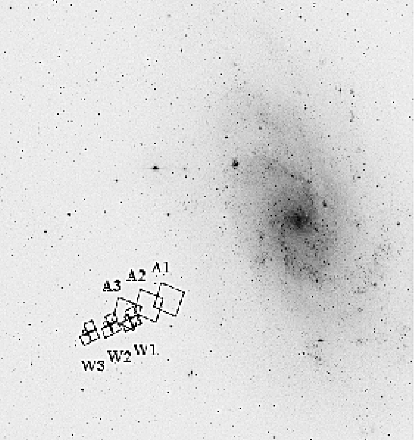
Figure 1.— Image showing M33 and the approximate locations and sizes of the regions observed with ACS and WFPC2. North is up and East is to the left. The image dimensions are $1\arcdeg$ on a side.

The data were retrieved from the Space Telescope Science Institute (STScI) after going through the standard CALACS pipeline and “on-the-fly” processing. This processing generated FLT images which were bias and dark subtracted and flat-fielded. Because ACS flat-fields are designed to flatten a source with uniform surface brightness rather than preserve total integrated counts, it was necessary to multiply the FLT images by the pixel area maps provided on the STScI website.

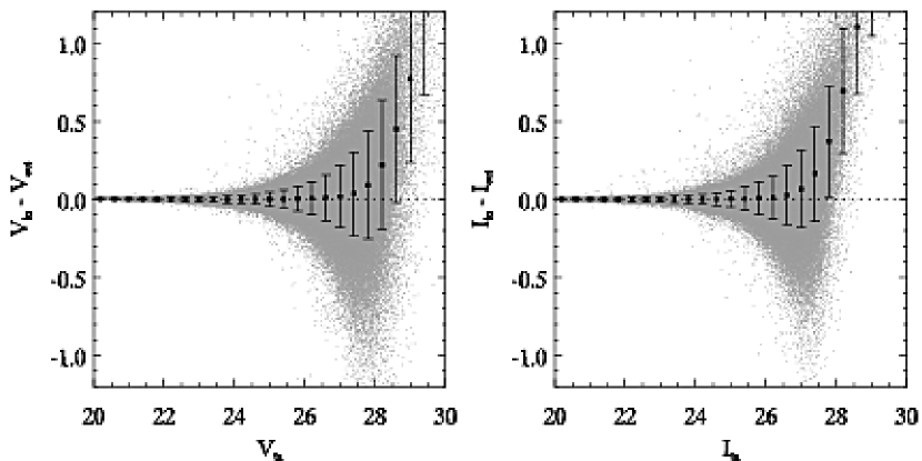
Figure 2.— The difference between input and output magnitude for all recovered artificial stars in field A1 (gray points). Each filled square and error bar gives the median error and its standard deviation.

Since these fields were sparsely populated, there were not enough bright stars to produce a point-spread function (PSF) with a sufficient signal-to-noise ratio. So an empirical high signal-to-noise ratio PSF was constructed from archival observations of the Galactic globular cluster (GGC) 47 Tuc. This PSF varied quadratically with position on the chips. We refer the reader to Sarajedini et al. (2006) for details of the PSF-making procedure. We found that PSF photometry resulted in color-magnitude diagrams (CMDs) with features that were more clearly defined than those resulting from small aperture photometry.

For each M33 field we first used Source Extractor (Bertin & Arnouts 1996) to identify sources, DAOPHOT to measure aperture magnitudes, and ALLSTAR to measure PSF magnitudes. This process was repeated on the resulting subtracted image to catch any stars that were missed. Then we input the star lists into DAOMASTER to derive precise spatial coordinate transformations between the frames in each filter. This allowed us to coadd all the frames to produce one single master image for each field. This master image was then run through two iterations of Source Extractor, DAOPHOT, and ALLSTAR as before. The resulting list of objects and individual CR-SPLIT exposures were input into ALLFRAME to obtain the final PSF magnitudes (Stetson 1987; Stetson & Harris 1988; Stetson 1993; Stetson 1994).

We derived mean aperture corrections from $\sim 50-100$ bright, isolated stars in A1. The standard deviations of the aperture corrections ranged from $0.02-0.03$ mag while the standard error of the mean was always $<0.01$ mag. There were not enough bright stars to derive reliable aperture corrections in A2 and A3. Since the ACS fields overlapped, we identified $\sim 200$ stars in common between A1 and A2 and $\sim 40$ between A2 and A3. From these stars we calculated mean offsets to bring the PSF magnitudes of A2 and A3 onto the same scale as A1. The standard deviation of each group of offsets was $\sim 0.05$ mag while the standard error of the mean was $<0.01$ mag. We applied the appropriate CTE corrections following the prescription in Riess & Mack (2004). These corrections were usually $<0.005$ mag.

To convert the aperture magnitudes to the standard $UBVRI$ system, we used the theoretical transformation of Sirianni et al. (2005). These authors quote an uncertainty of 0.05 mag for this transformation which we adopt as the uncertainty in the photometric zero-point in the present study.

To reduce spurious detections (e.g. incompletely masked cosmic rays, background galaxies, noise, etc.) we made cuts on the final catalog according to the following criteria. An object was kept if it was detected on all CR-SPLIT exposures, if $\chi<3\sigma$ of the median $\chi$ at its magnitude, $sharp<3\sigma$ of the median $sharp$ at its magnitude, $|sharp|\leq 0.5$, and $error<2$ times the median $error$ at its magnitude. The parameter $\chi$ measures the quality of the PSF fit and $sharp$ measures the sharpness or spatial extent of the object. There were 22415, 7666, and 3337 stars in the final catalogs for A1, A2, and A3, respectively.

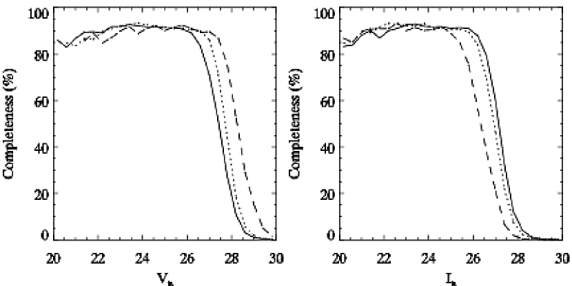
Figure 3.— Completeness rate as a function of input magnitude in field A1 for the input color ranges $-0.5<(V-I)<0.5$ (solid), $0.5<(V-I)<1.5$ (dotted), and $1.5<(V-I)<2.5$ (dashed).

We ran a series of extensive artificial star tests to accurately estimate the photometric errors and completeness rates. For each field, we generated two catalogs of artificial stars with known magnitudes. The magnitudes in the first catalog were chosen to mimic the observed distribution of stars in the CMD. Regions with no observed stars were assigned a minimum number of artificial stars to fully cover the CMD. The second catalog was compiled from the unscattered magnitudes of the model stars making up the synthetic CMDs described in Paper III. This ensured a more efficient and complete sampling of the error and completeness functions because it focused on regions where the true stellar colors and magnitudes are expected to lie. In total, $\sim 1\times 10^{6}$ artificial stars were generated for each field.

The artificial stars were inserted into the original frames using the same PSFs that we used to photometer the original frames. We placed the stars on a regular grid such that the spacing between them was 2.1 PSF fitting radii (42 pixels). This distance was chosen as a compromise between the requirement that the artificial stars not change the crowding conditions and the need for high computing efficiency. To fully sample the PSFs, we randomly varied the starting position of the grid and allowed for sub-pixel positions. The images were then photometered in exactly the same manner as before using exactly the same detection requirements.

In Figure 2 we show the difference between input and output magnitude as a function of input magnitude for all recovered stars in field A1. The gray points are the individual artificial stars while the black squares and error bars represent the median and standard deviation in bins 0.4 mag wide. This figure shows how a star is likely to get redistributed in the CMD if you know where it originates before the measurement process. For most of the magnitude range covered in each band, there is no significant difference between the input and output magnitudes. However, stars with input magnitudes $V_{in}\gtrsim 27.5$ or $I_{in}\gtrsim 27.0$ tend to be recovered brighter than their true magnitudes because measuring errors or random fluctuations in the unresolved background light may scatter faint stars below the detection limit (Stetson & Harris 1988; Gallart et al. 1995; Bellazzini et al. 2002b).

In Figure 3 we show the variation of the completeness rate with input magnitude and color for A1. The solid, dotted, and dashed lines correspond to the color ranges $-0.5<(V-I)<0.5$, $0.5<(V-I)<1.5$, and $1.5<(V-I)<2.5$, respectively. The completeness rises rapidly from the faint end and, due to our detection requirements and the presence of cosmic rays and bad pixels, levels off at $\sim 90\%$ at $V_{in}\sim 26.0$ and $I_{in}\sim 25.0$. The completeness rate reaches 50% at $V_{in}\sim 27.4-28.2$ and $I_{in}\sim 26.2-27.0$ depending on the color. The errors and completeness rates for A2 and A3 are similar to within $\pm 3\%$ over most of the magnitude range (i.e., crowding is not a strong limiting factor).

2.2. WFPC2

Parallel observations were also taken with the Wide Field and Planetary Camera 2 (WFPC2). The exposure times were 280 s in F606W and 1000 s in F814W divided into two CR-SPLIT exposures per filter. Fig. 1 shows the locations of the fields which will be referred to as W1, W2, and W3 in order of increasing galactocentric distance. Table 1 contains the exposure information.

We elected to use HSTphot (Dolphin 2000) rather than DAOPHOT to obtain PSF photometry. Our experience has been that the former is superior in computational efficiency but the latter is superior in photometric depth. Since the WFPC2 exposure times are relatively short the extra photometric depth gained by using DAOPHOT was not worth the extra computational time.

Photometry was obtained following the cookbook procedure in the HSTphot manual. In summary, bad pixels, cosmic rays, and hot pixels were masked and the two images in each filter were coadded. Then HSTphot was run with individual filter and total detection thresholds of $1\sigma$ and $2\sigma$, respectively. We enabled the options to refit sky and perform a weighted PSF fit which gives the central PSF pixels more weight during the fitting. To reduce spurious detections in the final catalogs we required $\chi<2.5$, $S/N>5$, and $|sharp|<0.5$. Even after these cuts we had to remove 72, 154, and 30 stars from the catalogs which were artifacts from the diffraction spikes of bright foreground stars. The final catalogs then contained 648, 429, and 433 stars.

3. Color-Magnitude Diagrams

The CMDs for A1 $-$ A3 are presented in Figures $\ref{fig:cmd_A1}-\ref{fig:cmd_A3}$. Qualitatively, they bear some resemblance to the CMDs of M33’s inner disk which were obtained with WFPC2 and presented in Sarajedini et al. (2000). The most prominent features in all three CMDs are the red clump (RC) at I $\sim$ 24.4 and red giant branch (RGB) whose brightest stars reach a color of $(V-I)\sim 2$. Field A1 also contains a significant blue plume of younger main sequence (MS) stars at $(V-I)\sim 0$ and a red supergiant (RSG) sequence (sometimes referred to as the “vertical clump”) extending from the top of the RC and adjacent to the RGB.

The CMD for field A1 is reproduced in Figure 7 with isochrones from Girardi et al. (2002) overplotted assuming a foreground reddening of $E(V-I)=0.06\pm 0.02$ (Mould & Kristian 1986; Sarajedini et al. 2000) and extinction $A_{I}=1.31E(V-I)$ (von Hippel & Sarajedini 1998) . The pair of isochrones overlapping the MS have a global metallicity [M/H] $=$ –0.7 and ages of 100 and 398 Myr. The three horizontal lines mark the MS positions of 5, 4, and 3 $M_{\sun}$ from top to bottom, respectively, for the 100 Myr isochrone. In A1, the brightest MS stars have masses close to $5\ M_{\sun}$. In A2 and A3 there are only a handful of possible MS stars with masses above $4\ M_{\sun}$ and $1-2$ dozen with masses in the range $3-4\ M_{\sun}$. The termination of the MS in A1 provides an upper limit of $\sim 100$ Myr to the ages of the youngest stars.

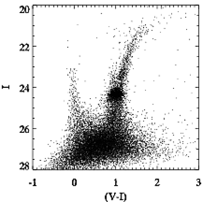
Figure 4.— CMD of field A1. The main features are the RC at I $\sim$ 24.4, the RGB extending from the RC to brighter magnitudes, and the blue plume of younger MS stars at $(V-I)\sim 0$.

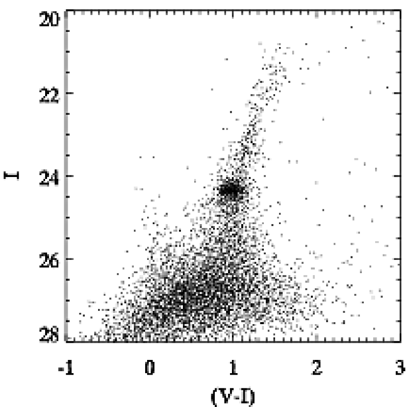
Figure 5.— Same as Fig. 4 but for field A2.

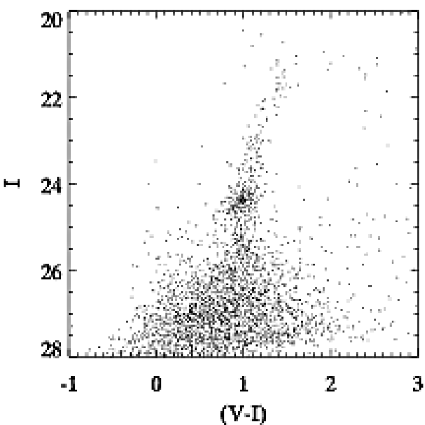
Figure 6.— Same as Fig. 4 but for field A3.

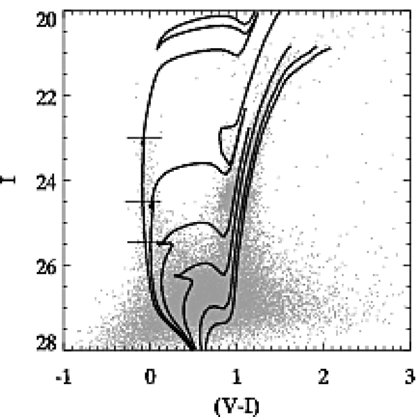
Figure 7.— CMD of A1 with isochrones from Girardi et al. (2002) overplotted. The isochrones have a metallicity of [M/H] $=-0.7$ and ages of 100 Myr, 398 Myr, and 1.0, 2.0, 5.0, and 7.9 Gyr from top to bottom, respectively. The three horizontal lines mark the 100 Myr MS locations of 5, 4, and 3 $M_{\sun}$ from top to bottom, respectively.

The mean color error at I $\sim$ 24 is only $\approx 0.05$ mag while the width of the MS at this magnitude is $\sim 0.2$ mag. This indicates an intrinsic color spread to the MS which could be due to a spread in metallicity, age, reddening or some combination thereof. A metallicity spread alone would have to be several tenths of a dex because the MS for [M/H] $=$ 0.2 is only $\sim$ 0.06 mag redder at I $=$ 24.0 than that for [M/H] $=$ –0.7. There is evidence for an age spread in the MS because a single age cannot simultaneously account for the bright MS turn-off and the presence of the RSG sequence extending from the top-left of the RC. The isochrones indicate the RSG sequence is probably a few hundred Myr older than the youngest MS stars. Sarajedini et al. (2006) estimated a typical disk reddening of $E(V-I)=0.3$ based on M33 RR Lyraes located at $R_{dp}\approx 13\arcmin$. Reddening values that large in field A1 would be surprising given that it is located almost 3 times farther out. However, little is known about the distribution of dust in M33 so we cannot rule out some contribution to the MS width due to dust.

The 2 $-$ 8 Gyr isochrones in Fig. 7 indicate an age spread of several Gyr could account for much of the RGB width. However, metallicity has a larger effect on the color of the RGB than age. Because of the well-known age-metallicity degeneracy, multiple combinations of age and metallicity are consistent with the position of the RGB. To get a rough idea of which ages and metallicities, we fit a Guassian to the color distribution of all stars in A1 with absolute magnitudes in the range $-3.7<M_{I}<-3.3$. The peak of the distribution lies at $(V-I)_{0}=1.53$ which we adopt as the dereddened value of the color index, $(V-I)_{0}^{-3.5}$. Figure 8 shows the result of comparing $(V-I)_{0}^{-3.5}$, which is the dashed line, with theoretical values extracted from the RGB loci of the Girardi et al. isochrones which are displayed as solid lines. The dotted lines represent the $1\sigma$ width of the observed distribution. Interpolating between the theoretical lines by eye we estimate that the bulk of the RGB stars in A1 could have metallicities in the range $-1.3<[M/H]<-0.8$ at an age of 14.1 Gyr and $-0.8<[M/H]<-0.4$ at 2 Gyr. These two ages are, respectively, the approximate maximum and minimum possible ages for first ascent RGB stars and are constrained by the age of the Universe and the time at which the RGB phase transition occurs (Ferraro et al. 1995; Barker et al. 2004). In A2 the consistent ranges are $-1.7<[M/H]<-0.8$ at 14.1 Gyr and $-1.1<[M/H]<-0.4$ at 2 Gyr. There are not enough stars in A3 to reliably fit a Gaussian using the same procedure. These limits are very approximate as we have only used the central 68% of the RGB stars. In addition, the presence of AGB stars could cause an underestimate of the metallicity because they lie just to the left of first-ascent RGB stars of the same age and metallicity. We have also only used a small portion of the RGB whose overall shape depends on chemical composition and age. Paper III has a more thorough analysis which includes these effects.

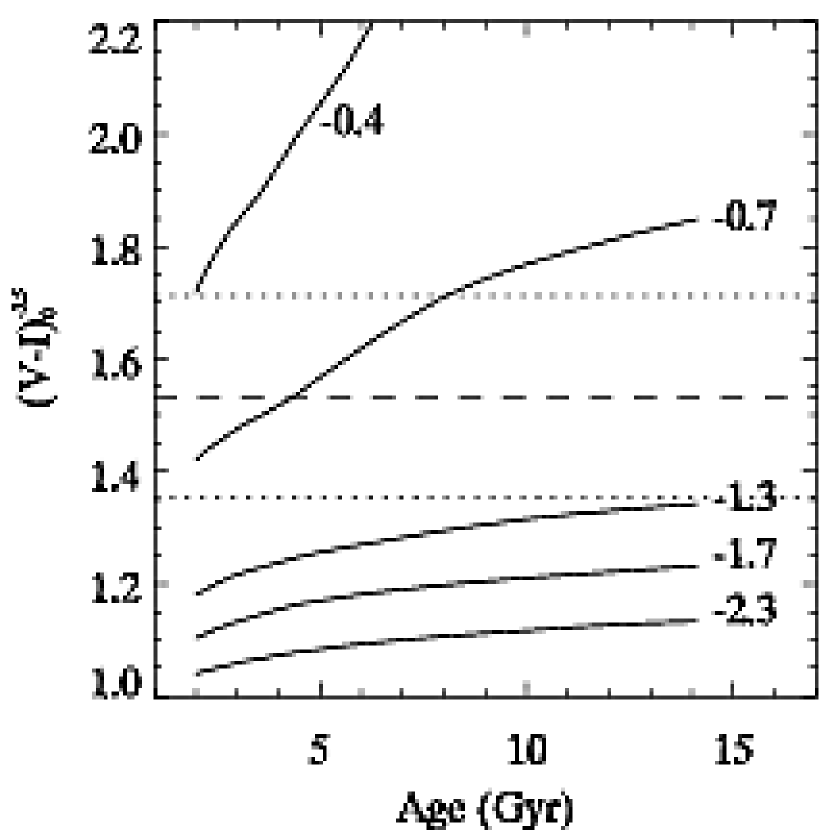
Figure 8.— Age and metallicity constraints from the dereddened color (dashed line) and width (dotted lines) of the RGB in A1. The solid lines are the predictions of the Girardi et al. (2002) isochrones.

The color and magnitude of the RC are also sensitive to the age and metallicity of its constituent stars. In Figure 9 we show a close-up of the RC region in A1 with mean theoretical values from Girardi & Salaris (2001) as a function of metallicity and age. The curves have metallicities of $-1.3$, $-0.7$, and $-0.4$ from left to right, respectively. The symbols on each curve represent 5 different ages. The open circles correspond to 1 Gyr, squares to 2 Gyr, triangles to 5 Gyr, stars to 8 Gyr, and filled circles to 12 Gyr. The cross shows the observed mean absolute magnitude ($-0.41$) and dereddened color ($0.94$). This figure provides evidence for the existence of stars $\sim 2-5$ Gyr old with a small dependence on metallicity. If the mean metallicity is $-0.7$ then an age of $\sim 5$ Gyr is preferred but if the metallicity is $-0.4$ then $\sim 2$ Gyr is preferred. The mean RC magnitude and color for A2 are, respectively, $-0.40$ and $0.92$ while for A3 they are $-0.38$ and $0.92$. This indicates that a similar intermediate-age population exists in the other fields, as well. This fact does not rule out the presence of older ages because as can be seen in the figure stars are observed throughout the entire region spanned by the models. Furthermore, the RC is biased toward younger ages because the core helium burning lifetime decreases with age (Girardi & Salaris 2001). Indeed, there is also a sequence of stars extending from the RC toward bluer colors and fainter magnitudes which lies just above the 12 Gyr point on the [M/H] $=$ –1.3 curve. With such few stars it is hard to say whether it is just a random grouping or the horizontal branch (HB) of an older and more metal-poor population. Finally, this figure also nicely shows that the left half of the RC can contain stars younger than 1 Gyr.

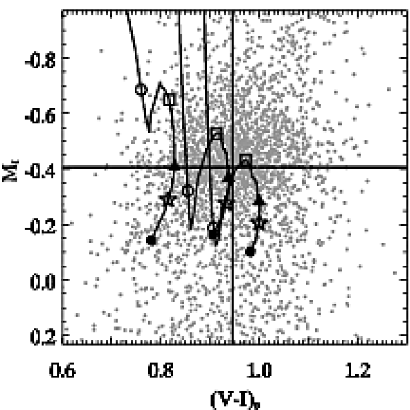
Figure 9.— RC region of A1 with mean theoretical RC values from Girardi & Salaris (2001) as a function of metallicity and age. The curves have global metallicities of $-1.3$, $-0.7$, and $-0.4$ from left to right, respectively. The open circles correspond to 1 Gyr, squares to 2 Gyr, triangles to 5 Gyr, stars to 8 Gyr, and filled circles to 12 Gyr. The cross marks the observed mean magnitude and color of the RC.

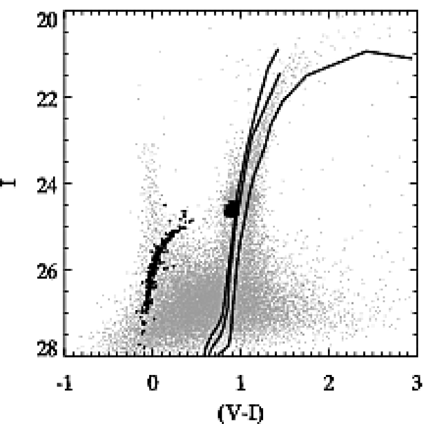
Figure 10.— CMD of A1 with the RGB ridge lines and HB loci of M92 ([Fe/H] = $-2.14$), NGC 6752 ([Fe/H] = $-1.54$), and 47 Tuc ([Fe/H] = $-0.70$) overplotted.

The RGB ridge lines of the GGCs M92, NGC 6752, and 47 Tuc from Brown et al. (2005) are overplotted on the CMD of A1 in Figure 10. The GGC data was originally in the ACS instrumental system but we have transformed them using the prescription and cluster parameters outlined in Brown et al. and using the same transformations that we applied to the M33 data. The GGC ridge lines span the width of M33’s RGB indicating that the oldest stars in A1 most likely have metallicities between [Fe/H] $=-1.54$ (NGC 6752) and $-0.70$ (47 Tuc). This empirical comparison is in agreement with what we found above using the Girardi et al. models and demonstrates that no serious errors have been introduced in the transformation to the ground-based filter system.

The HB loci of the same three GGCs are also plotted in Fig. 10. Stars in the blue HB tail at $(V-I)\sim 0$ belong to both M92 and NGC 6752 while the red HB at $(V-I)\sim 0.9$ belongs to 47 Tuc. The bulk of M33’s core helium burning stars are brighter than those of 47 Tuc providing further evidence for a population younger than the GGCs. However, as noted previously, the faintest portion of M33’s RC could contain stars as old as 47 Tuc. Because of its magnitude and color range, the young MS makes it difficult to confirm or rule out completely the presence of a blue HB tail in M33 similar to that of M92. However, it appears that any such population is likely to be a small fraction of the total core helium burning population at the present epoch since there is no significant overdensity of stars on the MS as would be expected from such a feature superposed on the MS. There are some stars located in the Hertzprung Gap between the MS and RC which could be blue HB stars, sub-giant branch (SGB) stars $\sim 1$ Gyr old, or foreground stars.

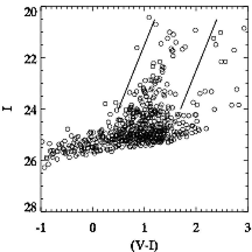
Figure 11.— CMD of field W1. Stars between the lines were used to study the stellar surface density.

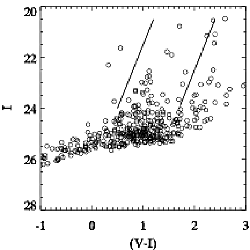
Figure 12.— Same as Fig. 11 but for W2.

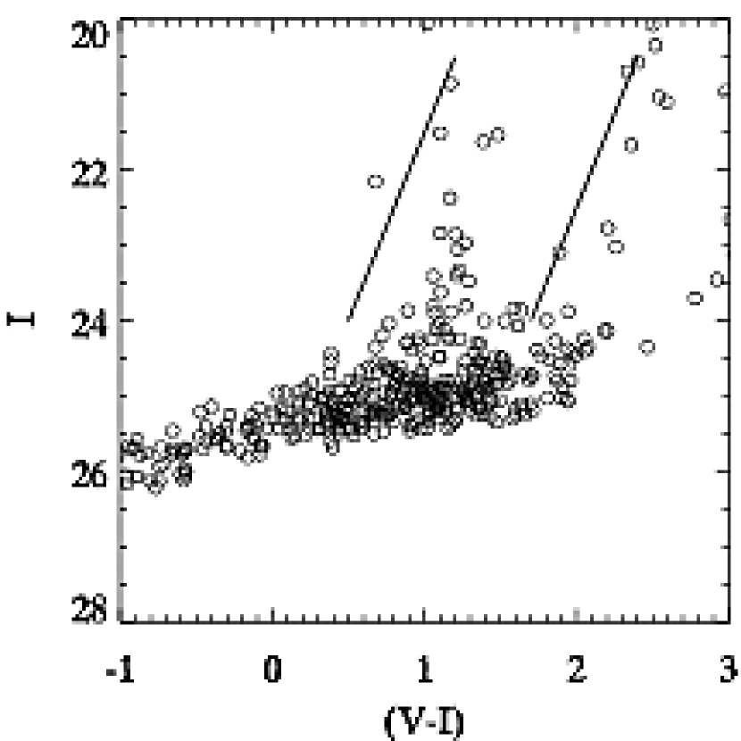
Figure 13.— Same as Fig. 11 but for W3.

Figures $\ref{fig:cmd_W1}-\ref{fig:cmd_W3}$ display the CMDs for the three WFPC2 fields. Due to the shorter exposure time in F606W, the limiting magnitude is about 2 magnitudes brighter than in the ACS fields. Most of the CMD features are washed out except for the RGB. Because of the shallower photometric depth and fewer number of stars, we do not use the WFPC2 CMDs in any part of this study except in the analysis of stellar surface density.

4. Stellar Surface Density

The spatial distribution of stars can yield insight into what type of population we are observing (i.e. disk, thick-disk, or halo). We show the surface density of RGB stars as a function of deprojected radius in Figure 14. The stars were selected to lie between the lines in Figs. $\ref{fig:cmd_W1}-\ref{fig:cmd_W3}$ (note that the lines are not shown in Figs. $\ref{fig:cmd_A1}-\ref{fig:cmd_A3}$ for clarity). Each ACS field was divided into four radial bins (represented by diamonds) whereas each WFPC2 field was treated in its entirety (represented by squares). Since W1 coincides with A3, the WFPC2 fields were brought onto the completeness scale of the ACS fields by normalizing the surface density in W1 to that in A3. This avoids making uncertain estimates of the differing completeness rates between the ACS and WFPC2 fields within the RGB selection region. However, using the raw WFPC2 densities does not change the results. Hence, W1 is not shown in Fig. 14 nor is it included in the fits below. The error bars reflect the Poisson uncertainty normalized by the actual area observed in each radial bin.

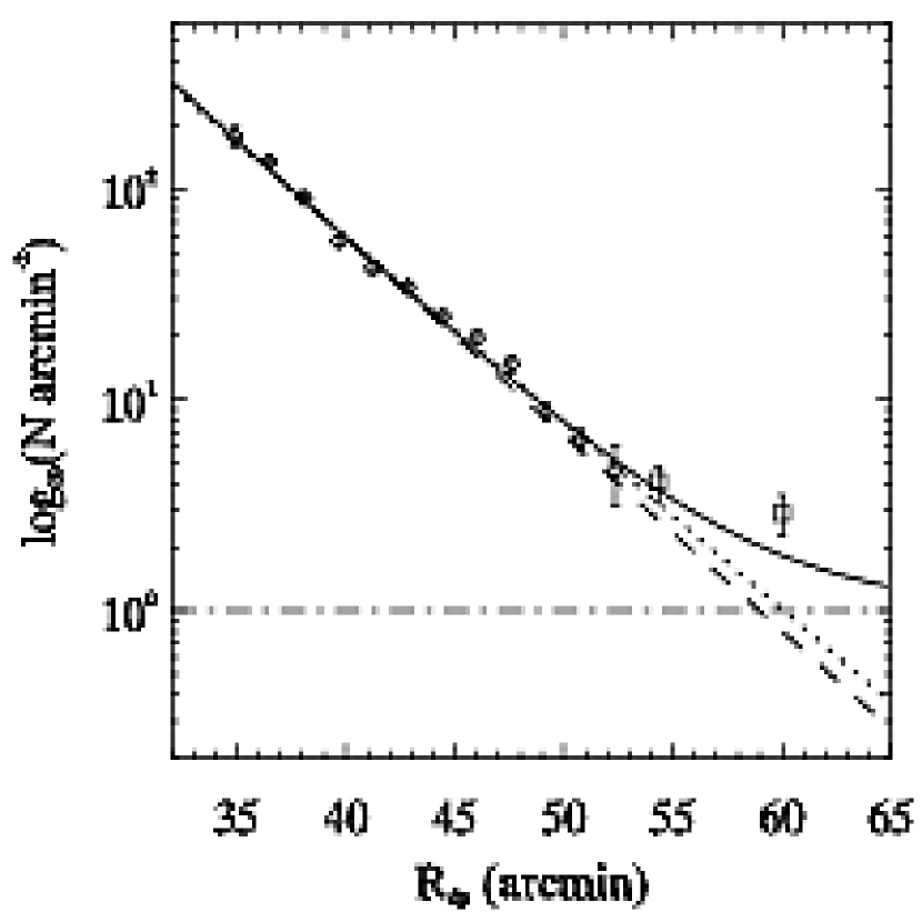
Figure 14.— Surface density of RGB stars as a function of deprojected radius. The diamonds correspond to fields A1 – A3 and the squares correspond to fields W2 and W3. The error bars are Poisson errors scaled by the area observed in each radial bin. The dotted line shows an exponential fit to all the points while the solid line shows an exponential plus constant model (dashed + dot-dashed).

Note that we have neglected error bars in deprojected radius due to the finite thickness of the disk. Seth et al. (2005) observed a sample of edge-on late-type spiral galaxies similar to M33 and found the vertical scale heights of their RGB stars to range from $\sim 200-700$ pc. If we take 500 pc as representative, then this translates to an uncertainty of $\pm 0.74$ kpc for M33. We have also assumed that the inclination and position angle are constant. Corbelli & Schneider (1997) fit a tilted-ring model to the HI distribution and found that the position angle changes from $\sim+20\arcdeg$ to $\sim-15\arcdeg$ over the region we have observed. Whether the stellar disk follows this change is unclear.

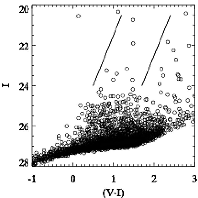
Figure 15.— CMD for a subsample of Hubble Deep Field images. Objects between the lines were used to estimate contamination from background galaxies and foreground stars.

An exponential profile was fit to the observed distribution in a least-squares sense and it is shown as the dotted line in Fig. 14. The scale length of the fit is $4.9\arcmin\pm 0.1\arcmin$. The surface density in W3 shows a significant ($3\sigma$) deviation from the exponential profile. To assess the level of contamination from background galaxies and foreground stars we reduced a subsample of images (2 in each filter) of the Hubble Deep Field using the same technique and thresholds that were applied to M33. The resulting CMD is shown in Figure 15 and contains 7 objects in the RGB selection region. Therefore, we estimate the surface density of background galaxies and foreground stars to be $\sim 1\ \rm arcmin^{-2}$. Including this constant offset in the fit reduces the exponential scale length to $4.7\arcmin\pm 0.1\arcmin$. The solid line in Fig. 14 represents the sum of the exponential (dashed) and offset (dot-dashed). The last point still shows an excess of stars but only at the $1.8\sigma$ level. If this excess is not due to Poissonian fluctuations then it could represent a transition to a more extended stellar component, a point to which we return later.

The K-band surface brightness scale length of M33 has been measured to be $5.8\arcmin-5.9\arcmin$ (Regan & Vogel 1994; Simon et al. 2006). When dealing with integrated light, the K-band is generally thought to be a better tracer of the stellar distribution than optical bands (but see Seth et al. (2005) for an alternative view). Regan & Vogel found a systematic decrease in the surface brightness scale length with wavelength. They used a simple toy model which ascribed this trend to the absorbing effects of dust. Their model neglected the effects of forward scattering and variations in stellar age and abundance but predicted that the true scale length of the stellar disk is $5.3\arcmin$.

Our estimate of the scale length is a more direct measurement of the underlying stellar structure and is free from many of the systematic uncertainties affecting surface photometry including dust absorption and scattering. However, it should be noted that we have sampled a small region outside that studied by Regan & Vogel and Simon et al. Hence, if M33’s density profile is not a single exponential then the difference between our measurements and theirs would be expected. Rowe et al. (2005) surveyed M33’s luminous stellar populations and found a clear break in the carbon star profile at $R_{dp}\approx 35\arcmin$. While they did not make any exponential fits to their profile we estimate by eye that outside this radius the scale length of their profile is remarkably close to our result. This picture is confirmed by Ferguson et al. (2006) who conducted a wide field survey of M33 with the INT 2.5-m telescope. They report a similar break in the RGB density profile at about the same radius found by Rowe et al. and beyond which the scale length is similar to what we have found.

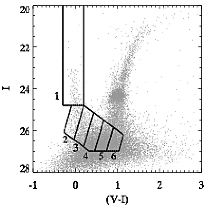
Figure 16.— CMD of A1 and the six boxes used to study the age dependence of the radial scale length.

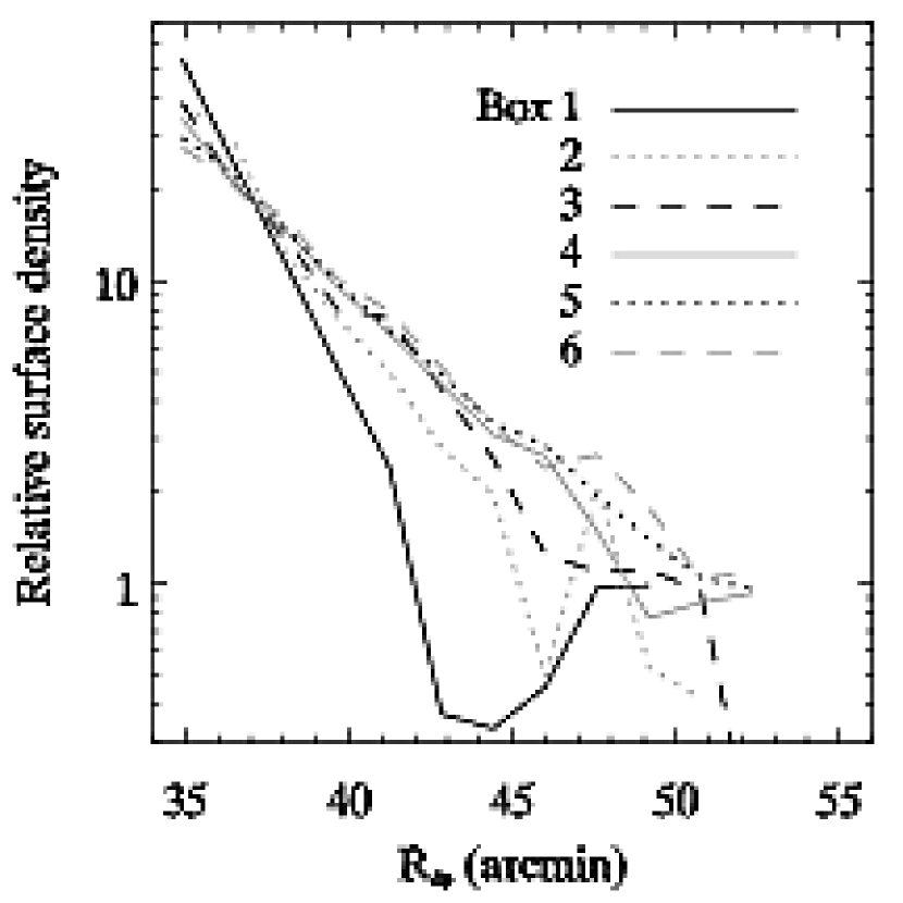
Figure 17.— Relative surface density of stars in each box shown in Fig. 16.

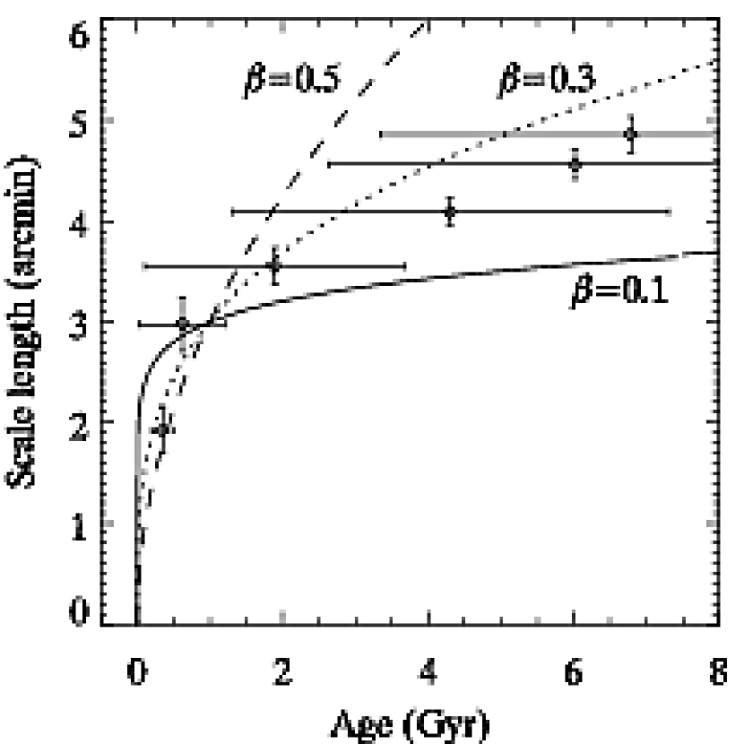
Figure 18.— Disk scale length as a function of age. Each point and horizontal error bar is the mean and standard deviation of stellar ages for each box shown in Fig. 16. The vertical error bars are the random uncertainties in the scale lengths from the least-squares fits. Three arbitrary power-law relations where $h=3t^{-\beta}$ are shown for comparison.

In Paper I, we found that massive MS stars were more concentrated toward M33’s nucleus than AGB stars which in turn were more concentrated than RGB stars. This implied a progression in the stellar scale length with age. Inspection of the CMDs presented here also suggests that the density of stars in the young MS declines faster than the density of RGB stars. To investigate this in more detail we selected several regions of the CMD on the basis that each region probes different age ranges. Using the results of Paper III we found that contours of constant age run roughly diagonally since the main sequence turnoff and sub-giant branch move toward fainter and redder magnitudes with age. Figure 16 shows the regions we selected. The boundaries were chosen to roughly follow lines of constant age and the sizes were chosen as a compromise between the need for good number statistics and a small range of ages in each box. The faint limit was chosen to avoid the region where systematic magnitude errors dominate and to minimize contamination from non-stellar sources. Gallart et al. (1999) used a similar approach to isolate different age ranges in studying the star formation history of Leo I. Table 2 lists the mean age (averaged over all three fields) and scale length for each box and their standard deviations.

Table 2Variation in Scale Length With Age

Box	Age	$\sigma$	$h$	$\sigma$
	(Gyr)	(Gyr)	(arcmin)	(arcmin)
1	0.35	0.15	1.92	0.22
2	0.62	0.58	2.98	0.27
3	1.90	1.79	3.55	0.18
4	4.31	3.00	4.09	0.14
5	6.02	3.40	4.56	0.14
6	6.79	3.45	4.86	0.18

In Figure 17 we show the relative stellar surface density of each box for fields A1 $-$ A3. There is a trend of decreasing concentration as the boxes get fainter, and, hence, older. We fit an exponential profile to each box’s stellar distribution spanning all three fields. Figure 18 displays the behavior of the scale length with mean age. The curved lines show three power-law relations of the form $h=3t^{-\beta}$ with $\beta=0.1,0.3,0.5$. The form of these relations is somewhat arbitrary and we show the curves only for reference. The vertical error bars are the statistical uncertainties in the scale length from the least-squares fitting procedure. The horizontal error bars represent the spread of the ages in each box. The precise ages probably represent the largest source of uncertainty in this plot. The y-errors are fairly uniform but the x-errors increase dramatically for the oldest boxes. This is because the stellar isochrones get more photometrically degenerate with age. Comparison of the power-law relations suggests that $0.1\lesssim\beta\lesssim 0.3$ but we refrain from making a more precise estimation due to the inherent systematic uncertainties. We discuss possible interpretations in §7.

5. Metallicity Distribution Functions

Following the analysis in Paper I, we employ the Saviane et al. (2000) grid of RGB fiducials to construct the metallicity distribution function (MDF) of each field. Those authors used a large homogeneous photometric database of GGCs to derive a function which has one parameter, [Fe/H], that specifies the shape of the RGB. If an RGB star’s absolute magnitude and dereddened color are known, then the function can be solved for the star’s metallicity. To minimize contamination from foreground stars, AGB stars, and red supergiants, we restrict the present analysis to stars in the region $1.0\leq(V-I)_{0}\leq 2.2$ and $-3.9\leq M_{I}\leq-2.4$. The total number of stars in the selected CMD region is 207 in A1, 84 in A2, and 34 in A3.

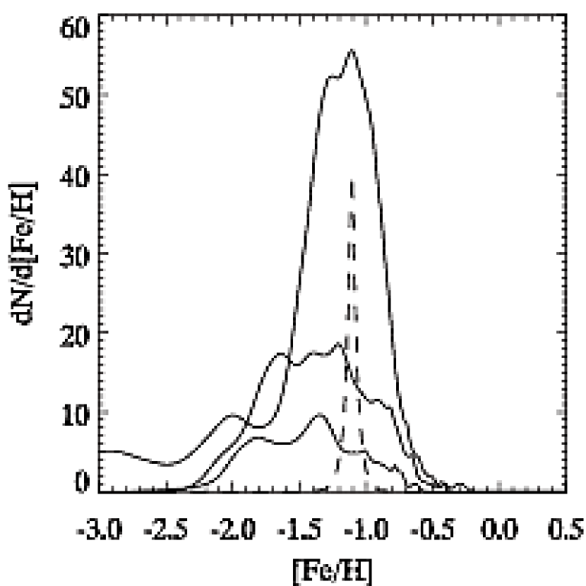
Figure 19.— Generalized histogram of the RGB metallicity distribution function in field A1 (top), A2 (middle), and A3 (bottom). The dashed curve shows the “instrumental response.”

The resulting MDFs for A1 $-$ A3 are displayed in Figure 19 as the solid-line generalized histograms from top to bottom, respectively. These were constructed by assigning a unit Gaussian to each star with a standard deviation equal to the star’s metallicity uncertainty. The median metallicity is $-1.14$, $-1.23$, and $-1.30$ while the interquartile range is 0.4, 0.6, and 0.6 dex. The dashed line represents the “instrumental response,” namely the recovered distribution for a test population having a single metallicity (Bellazzini et al. 2002a). The test population consisted of 2000 stars whose input magnitudes reproduced the observed RGB luminosity function and whose colors reproduced the Saviane et al. RGB ridge line for [Fe/H] $=-1.1$. The standard deviation of the recovered distribution is 0.04 dex and represents the total intrinsic random error introduced during the entire measuring process from the photometric reduction to the measurement of metallicities. We find that when the $1\sigma$ uncertainties in the distance and reddening are added in quadrature they introduce a systematic error of $\sim 0.1$ dex.

6. Metallicity Gradient

We are interested in tracing out the extent of M33’s disk. To do so we must place the results of the previous section in the context of other studies. We have culled from the literature a list of RGB metallicity measurements in M33 using similar techniques. Figure 20 summarizes these other measurements. The open triangle is based on the results of Stephens & Frogel (2002, SF02) who imaged the central 22$\arcsec$ of M33 with Gemini North. They obtained near-IR photometry and from the slope of the RGB calculated a mean metallicity of $-0.26\pm 0.27(rand)$. The filled circles are the results of Kim et al. (2002, K02), who obtained VI photometry of 10 WFPC2 fields located throughout the disk ($R_{dp}\sim 1-6$ kpc). They found median metallicities ranging from $-0.6$ to $-0.9$ with a typical error of 0.09 dex. It is not clear whether their quoted errors are random or systematic. The open circles correspond to the results of Galleti et al. (2004, G04), who obtained VI photometry of two fields to the NW of M33’s nucleus. In both fields they found a median metallicity of $-1.03\pm 0.40$ where the error represents the “instrumental response.” The filled squares are the results of Paper I (PI) after applying a missing factor of cos(DEC) in the original calculation of deprojected radii. The error bars demonstrate the “instrumental response.” A large survey covering projected radii of $26\arcmin-60\arcmin$ was conducted by Brooks et al. (2004, B04) who found a peak metallicity of $-1.27\pm 0.04(rand)$ which is shown as the open (downward-pointing) triangle. Davidge (2003, D03) imaged a field at $R_{dp}\approx 72\arcmin$ and found evidence for an excess number of stars relative to a control field which he intrepreted as AGB and RGB stars in M33. He measured the RGB metallicity to be [Fe/H] $=-1.0\pm 0.3(rand)\pm 0.3(sys)$ which is shown as an open square. We show only the random error to be more consistent with the other points. The filled triangles represent the results of the present study while the errors are the “instrumental response” discussed in the previous section.

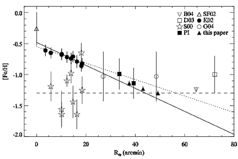
Figure 20.— RGB metallicity gradient in M33. The dotted and solid lines are, respectively, the fits from K02 to all the filled circles and all but the inner two where crowding was severe. The dashed line represents M33’s halo metallicity (see text for details).

The star symbols in Fig. 20 correspond to 9 halo globular clusters of M33. Their metallicities were estimated by Sarajedini et al. (2000, S02) using WFPC2 VI photometry and the slopes of the cluster RGBs. The errors for the clusters are random errors propagated through the relations between RGB color, slope, and metallicity. The mean metallicity of these clusters is $-1.27\pm 0.11(rand)$. Recently, Sarajedini et al. (2006) studied the RR Lyrae (RRL) population in an ACS field located at $R_{dp}\sim 15\arcmin$. They found that the RRL metallicity distribution exhibited a pronounced peak at [Fe/H] $\sim-1.3$ which they interpreted as evidence for a field halo population. The dashed line in Fig. 20 therefore represents the halo of M33 (including clusters and field stars).

M33’s disk presumably has a different star formation history from its halo so a transition from one to the other could be observable as a change in the apparent RGB metallicity gradient. The dotted line in Fig. 20 is the fit to the inner disk fields (filled circles) from K02 while the solid line is their fit which excluded the innermost two fields where crowding was severe. We stress that these fits were made independent of the other metallicity measurements. In Paper I, we found that the metallicity gradient was consistent with the inner disk gradient. In the present study we find that the same gradient extends out to $R_{dp}=50\arcmin$. Past this radius there appears to be a flattening in the gradient but the situation is somewhat uncertain. B04 interpreted their field to be dominated by a halo population because of the shallow surface density profile with a power-law slope of $-1.47$ and because their metallicity matched the halo globular clusters. Likewise, D03 suggested the asymptotic giant branch and RGB stars he found were the field counterparts to the halo globular clusters which may have formed over a timescale of several Gyr (see also S00). Unfortunately, these analyses relied heavily upon the adopted level of contamination from foreground Galactic stars and background galaxies. Only more precise measurements of RGB metallicities at radii past $R_{dp}=60\arcmin$ could determine if the disk gradient continues outward or if the slope flattens out as might be expected for a halo (or thick-disk) population. Such measurements could require large areas to obtain a statistically significant sample of RGB stars.

Finally, there are several important considerations to note while examining Fig. 20. First, we have used our fiducial M33 distance, inclination, and position angle and the centers of the fields studied to determine their deprojected distances. Because the D03, B04, and G04 fields were relatively large, it would be more accurate to plot their positions according to the mean RA and DEC of the RGB stars in their fields. Depending on the geometry of their fields relative to M33’s nucleus, this could have the effect of moving them inward to smaller radii because of the negative stellar density gradient.

Most importantly, all of the measurements presented in Fig. 20 compared M33’s RGB stars to the GGCs which are old ($\sim 12$ Gyr) and contain enhancements in the $\alpha$-element abundance ($\rm[\alpha/Fe]\sim 0.3$). As pointed out by Salaris & Girardi (2005), the RGBs of galaxies with composite stellar populations, such as the LMC and SMC, are often dominated by stars significantly younger than the GGCs with $\rm[\alpha/Fe]\sim 0.0$. Hence, the metallicities of such systems derived using the GGCs as fiducials could be underestimated by several tenths of a dex. Indeed, in Paper III we model the star formation history of fields A1  $-$  A3 using stellar evolutionary tracks with $\rm[\alpha/Fe]=0.0$ and we find that the true metallicity is $\sim 0.4$ dex higher but the metallicity gradient through the fields is roughly unchanged. From the Girardi et al. isochrones we estimate that approximately half of this offset is due to the lower $\alpha$-element abundance and half is due to a younger mean age ($\sim 6-8$ Gyr). If the outer regions were as young as 2 Gyr, the total offset would amount to $\sim 0.6$ dex. Currently there is no information on the star formation history of M33’s inner disk so it is possible the RGB metallicity gradient over its entire disk is shallower or steeper. However, it is unlikely that an age gradient can mimic the apparent metallicity difference of $\sim 0.8$ dex between M33’s central and outer regions because the latter are not young enough.

7. Discussion

It has been observed that many spiral galaxies exhibit a sharp drop in star formation across their disks, as measured by the surface brightness of the $H\alpha$ recombination line. The location of this drop, $R_{*}$, often occurs close to where the gas surface density falls below a theoretically defined critical density required for star formation. The nature and dependence of this threshold density on the local environment is not exactly clear. Kennicutt (1989) and Martin & Kennicutt (2001) argue that it is governed by gravitational instability as parameterized by the Toomre Q parameter. This parameter depends on the local epicyclic frequency and gas velocity dispersion. It accurately predicts the critical radius for many high surface brightness galaxies but fails for some low-mass spirals like M33 ($R_{*}=29\arcmin$) where large portions of the disk are below the threshold gas density but actively forming stars.

Corbelli (2003) used measurements of the gas kinematics in M33 to derive an extensive rotation curve and mass model. She found that the Toomre criterion could correctly predict $R_{*}$ in M33 if the surface density of either the stellar disk or dark matter was added to the gas density. Alternatively, a stability criterion based on the shear rate with a low gas velocity dispersion could also correctly predict $R_{*}$. However, such a modified criterion does not work as well for most other galaxies (Martin & Kennicutt 2001).

What implications do our results have for the star formation threshold in M33? We noted in §3 that field A1 contains stars $\approx 3-5\ M_{\sun}$ while A2 and A3 contain stars $\approx 3-4\ M_{\sun}$. These massive stars can be no older than their MS lifetimes of $\sim 100-400$ Myr and unless we have coincidentally observed them at the end of their MS phases then they are probably even younger. This fact is direct evidence for recent star formation at $R_{dp}\approx 35\arcmin-50\arcmin$ in apparent disagreement with M33’s star formation threshold radius of $29\arcmin$. It is possible that these massive stars actually formed at smaller radii and have since migrated outward. Given their young ages, however, there probably has not been sufficient time for this to occur.

Could star formation be ongoing today in our fields? Boissier et al. (2006) used GALEX images to study the radial variation of star formation in 43 spiral galaxies. Included in their sample was M33 whose Far-UV profile extended out to $R_{dp}\sim 43\arcmin$, well past the threshold radius measured with $H\alpha$. Indeed, nearly all of the galaxies in their sample displayed similar behavior leading to the conclusion that star formation is ongoing today in the outskirts of these galaxies but at levels too low to produce any ionizing stars. The UV continuum, however, is sensitive to the star formation rate integrated over the last 100 Myr. In contrast, the $H\alpha$ observations trace the star formation rate over the last 20 Myr (Kennicutt 1998). Therefore, it is possible that there are no ionizing stars alive today because star formation ended $20-100$ Myr ago.

This latter sencario could explain our observations of young stars in M33’s outskirts beyond the $H\alpha$ threshold radius and, therefore, save the applicability of the Toomre Q parameter to M33. However, we would still need to explain how star formation could have occurred at all so recently despite the low disk densities in these regions. Was the disk density in the recent past above the threshold density? To answer this we need to know the current densities of the gas, stars, and dark matter.

According to the tilted-ring model of Corbelli (2003) the azimuthally averaged HI column density is $\sim 3.0$, $2.0$, and $1.5\ M_{\sun}\rm\ pc^{-2}$ at the central radii of fields A1, A2, and A3, respectively. Complexities in the HI distribution can cause systematic and random errors when performing azimuthal averages even in detailed tilted-ring models. Such is the case in M33’s outer disk where residuals between the model and observed flux at different position angles within a ring can vary by a factor of $\sim 2$ (Corbelli & Schneider 1997). Azimuthally averaged column densities are what are commonly reported in the literature for other galaxies so we use them here as well. The high resolution aperture synthesis map of Newton (1980) shows that the HI density throughout our fields is below the lowest contour which corresponds to $\approx 4.3\ M_{\sun}\rm\ pc^{-2}$.

The amount of molecular gas in our fields is difficult to ascertain but it is unlikely to contribute significantly to the total gas content. Our fields lie outside the GMC survey of Engargiola et al. (2003) and are at the limit of the sensitivity and coverage of the CO maps presented by Heyer et al. (2004). The outermost reliable point in their map is at $R_{dp}\sim 24\arcmin$ where the $H_{2}$ column density is $\sim 0.6\ M_{\sun}\ \rm pc^{-2}$. This can be taken as a rough upper limit for our fields considering that the CO to $H_{2}$ conversion factor may be different in the outer disk where the metallicity is lower.

A crucial point to consider is whether the gas density in our fields could have been significantly greater just a few hundred Myr ago. This possibility is actually ruled out by the low star formation rate required to explain the small number of young, massive stars observed. From the star formation histories calculated in Paper III, we find that the mean star formation rate in the past 400 Myr has been $<0.04\ M_{\sun}\ \rm pc^{-2}\ Gyr^{-1}$. Thus, no more than $0.02\ M_{\sun}\ \rm pc^{-2}$ could have been converted to stars in that time.

Corbelli (2003) calculated the variation in the threshold density with radius in M33. According to her plots, the Toomre criterion predicts a threshold disk density that drops from $\sim 7$ to $6\ M_{\sun}\ \rm pc^{-2}$ across fields A1  $-$  A3 whereas the shear rate criterion predicts a threshold that is approximately constant at $\sim 5\ M_{\sun}\ \rm pc^{-2}$. Therefore, a few hundred Myr ago the gas density was below either threshold. Corbelli’s mass model predicts the gas to dominate the baryonic mass in these outer regions so it is also unlikely that the stellar mass contributes significantly to the total disk surface density. On the other hand, the dark matter density within the disk is about equal to the gas density. Hence, including dark matter in the total disk density can explain the recent star formation in field A1 but not A2 or A3.

A growing body of evidence has suggested that a constant threshold gas density of $\sim 3-10\ M_{\sun}\rm\ pc^{-2}$ describes the extent of star forming disks equally well if not better than a radially varying threshold like the Toomre Q parameter or shear rate criterion (Skillman 1987; Taylor et al. 1994; Ferguson et al. 1998; Martin & Kennicutt 2001). The physical basis for such a threshold could be related to the minimum pressure needed for the formation of a cold gas phase in the ISM (Elmegreen & Parravano 1994, Schaye 2004). If such a constant threshold applies to M33 then our results imply it is $\lesssim 3\ M_{\sun}\ \rm pc^{-2}$ and could be as small as $\sim 1\ M_{\sun}\ \rm pc^{-2}$. Indeed, Boissier et al. (2006) trace M33’s Far-UV profile out to gas densities of $\sim 1-2\ M_{\sun}\ \rm pc^{-2}$.

We now return to our finding that the stellar scale length increases with age. This result raises several interesting questions. Does this reflect something fundamental about M33’s collapse history? Does it arise from the progression of star formation on galactic scales? Or is it a by-product of subsequent dynamical processes which act to redistribute stars after they are formed?

In the common picture of inside-out galaxy formation the scale length of all stars and stellar remnants increases as the disk builds up to the present day size (e.g.  Naab & Ostriker 2006). This means that the oldest stars we observe today should have the smallest scale length in contrast to our results which show the opposite trend in M33. This seems to suggest an outside-in formation scenario.

A different interpretation is that we are observing a transition between two distinct components in M33, like a disk/thick-disk or disk/halo. This would explain why the number of RGB stars in field W3 is larger than predicted by a simple exponential plus constant model. If this is correct, then field A3 could have a non-negligible thick-disk/halo component which might explain why its metallicity is close to that of M33’s halo. Interestingly, the M-star profile measured by Rowe et al. (2005) shows a flattening at approximately the same location as fields A2 $-$ A3 further hinting at a second, more extended component.

M33’s halo was recently isolated kinematically by McConnachie et al. (2006) who analyzed Keck DEIMOS spectra of 280 stars located $\sim 38\arcmin$ along the major axis. These authors found evidence for three distinct kinematic components: a disk, halo, and an intermediate component which they hypothesized could be a tidal stream in M33. It is unclear how the intermediate component would affect our results because, if it is a stream, it might not go through our fields. The halo component, however, would be present in our fields although it’s precise contribution is uncertain. Our fields lie at about the same deprojected distance as those observed by McConnachie et al. but they are on the minor axis so the halo-to-disk ratio could be larger depending on the true halo density distribution.

Complicating the picture is the possibility of disk orbital heating mechanisms. These processes must, at some level, modify the stellar age, metallicity, and density gradients put in place by star formation regardless of whether it progresses inside-out or vice-versa. (e.g., L$\rm\acute{e}$pine et al. 2003, Sellwood & Binney 2002, Wielen et al. 1996). The classical mechanism involves gravitational encounters between stars and giant molecular clouds of mass $\sim 10^{6}\ M_{\sun}$ (Spitzer & Schwarzschild 1953). This process has been shown to heat the stellar disk at a rate where the vertical and radial velocity dispersions are related by $\sigma_{z}\propto\sigma_{R}\propto t^{-\alpha}$ where $\alpha\approx 0.25$ and $\sigma_{z}/\sigma_{R}\approx 0.7$ (Lacey 1984, Villumsen 1985). Unfortunately, observations in the Galaxy indicate that 1) there are too few GMCs with the requisite mass (Lacey 1984), 2) $\alpha\approx 0.5$ (Wielen 1977), and 3) $\sigma_{z}/\sigma_{R}\approx 0.5$ (H$\rm\ddot{a}$nninen & Flynn 2002). In response, other mechanisms have been proposed, from heating by spiral arms to massive halo black holes passing through the disk (Lacey & Ostriker 1985). The former is most promising because theoretical simulations predict $0.2\lesssim\alpha\lesssim 0.5$ for the resulting heating rate (De Simone et al. 2004). It’s biggest problem, though, is that spiral waves have no effect on the heating rate in the vertical direction and, thus, cannot explain why the heating rate has the same time dependence in the radial and vertical directions. It now appears that some combination of these processes takes place with spiral waves doing most of the heating and GMCs redistributing some of the radial peculiar velocities into the vertical direction (e.g., Carlberg 1987). The precise relative contributions could depend on the characteristics of the galaxy in question, like the mass spectrum of GMCs and the strength, number, pitch angle, and lifetime of spiral arms and other irregularities in the potential like bars and accreted satellites.

An important piece of the puzzle comes from Seth et al. (2005). After analyzing the vertical distribution of stars in six late-type spirals they found that the scale height increases for successively older stellar populations in a manner such that the power-law exponent $\beta<0.3$. For an isothermal disk, the vertical scale height is proportional to the vertical velocity dispersion. Seth et al. used this proportionality to show that if orbital diffusion is responsible for their results then the heating rate in the vertical direction must be significantly less than in the Galaxy, namely $\alpha<0.15$. These results are intriguingly similar to what we have found in M33 for the radial direction and point to a common origin in all late-type spirals.

8. Conclusions

We have presented deep VI photometry of three fields in M33’s outskirts at deprojected radii of $4-6$ visual scale lengths. The CMDs reveal a mixed stellar population with ages ranging from $\lesssim 100$ Myr to at least several Gyr. The presence of such young stars so far out in this galaxy is consistent with a low global star formation threshold. Assuming our fields are representative of all position angles at similar deprojected radii in M33, we argue that the threshold cannot be significantly more than the present-day azimuthally averaged gas surface density of $1-3\ M_{\sun}\ \rm pc^{-2}$ which is roughly consistent with, but on the low end of, theoretical expectations and previous measurements in other galaxies.

The metallicity gradient as inferred by comparing the observed RGBs to the GGCs is consistent with M33’s inner disk gradient traced by several other studies. The radial surface density of RGB stars declines exponentially with a scale length of $4.7\arcmin\pm 0.1\arcmin$. The scale length increases with age in a roughly power-law fashion with an exponent that is constrained to be $0.1\lesssim\beta\lesssim 0.3$. This behavior is similar to that found for the vertical scale height in a sample of late-type spiral galaxies like M33 (Seth et al. 2005). We are unable to say whether this behavior is due to the orbital diffusion of stars as they age or to intrinsic variations in star formation history with radius.

Given the exponential radial distribution, metallicity gradient, and mixed ages present in our fields it is likely they belong predominantly to M33’s disk. This would mean that M33’s disk extends out to at least $R_{dp}=13$ kpc, or $\sim 6$ V-band scale lengths. However, we cannot rule out the presence of a small, extended component like a thick-disk or halo particularly in the outermost field. This possibility can be tested with kinematics and by extending the metallicity measurements in M33 beyond this region to see if its gradient changes.

References

- (1)
- (2) Barker, M. K., Sarajedini, A., Geisler, D., Harding, P., & Schommer, R. 2007, AJ, in press
- (3) Barker, M. K., Sarajedini, A., & Harris, J. 2004, ApJ, 606, 869
- (4) Bellazzini, M., Ferraro, F. R., Origlia, L., Pancino, E., Monaco, L., & Olivia, E. 2002a, AJ, 124, 3222
- (5) Bellazzini, M., Fusi Pecci, F., Montegriffo, P., Messineo, M., Monaco, L., & Rood, R. T. 2002b, AJ, 123, 2541
- (6) Bertin, E., & Arnouts, S. 1996, A&AS, 117, 393
- (7) Boissier, S., Gil de Paz, A., Boselli, A., Madore, B. F., Buat, V., Cortese, L., Burgarella, D., Munoz Mateos, J. C. M., Barlow, T. A., Forster, K., Friedman, P. G., Martin, D. C., Morrissey, P., Neff, S. G., Schiminovich, D., Seibert, M., Small, T., Wyder, T. K., Bianchi, L., Donas, J., Heckman, T. M., Lee, Y., Milliard, B., Rich, R. M., Szalay, A. S., Welsh, B. Y., Yi, S. K. 2006, ApJS, in press
- (8) Brooks, R. S., Wilson, C. D., & Harris, W. E. 2004, AJ, 128, 237
- (9) Brown, T. M., Ferguson, H. C., Smith, E., Kimble, R. A., Sweigart, A. V., Renzini, A., Rich, M. R., & VandenBerg, D. A. 2005, AJ, 130, 1693
- (10) Carlberg, R. G. 1987, ApJ, 322, 59
- (11) Corbelli, E. 2003, MNRAS, 342, 199
- (12) Corbelli, E., Schneider, S. E. 1997, ApJ, 479, 244
- (13) Dalcanton, J. J., Yoachim, P., & Bernstein, R. A. 2004, ApJ, 608, 189
- (14) de Grijs, R., Kregel, M., & Wesson, K. H. 2001, MNRAS, 324, 1074
- (15) De Simone, R., Wu, X., & Tremaine, S. 2004, MNRAS, 350, 627
- (16) de Vaucouleurs, G. 1963, ApJS, 8, 31
- (17) Dolphin, A. E. 2000, PASP, 112, 1383
- (18) Elmegreen, B. G., & Parravano, A. 1994, ApJ, 435, L121
- (19) Engargiola, G., Plambeck, R. L, Rosolowsky, E., & Blitz, L. 2003, ApJS, 149, 343
- (20) Ferguson, A., Irwin, M., Chapman, S., Ibata, R., Lewis, G., Tanvir, N. 2006, astro-ph/0601121
- (21) Ferguson, A. M. N., Wyse, R. F. G, Gallagher, J. S., & Hunter, D. A. 1998, ApJ, 506, L19
- (22) Ferraro, F. R., Fusi Pecci, F., Testa, V., Greggio, L., Corsi, C. E., Buonanno, R., Terndrup, D. M., & Zinnecker, H. 1995, MNRAS, 272, 391
- (23) Ferreras, I., Silk, J., Boehm, A., & Ziegler, B. L. 2004, MNRAS, 355, 64
- (24) Freeman, K. C., & Bland-Hawthorne, J. 2002, ARA&A, 40, 487
- (25) Gallart, C., Aparicio, A., & Vílchez, J. M. 1995, AJ, 112, 1928
- (26) Gallart, C., Freedman, W. L., Aparicio, A., Bertelli, G., Chiosi, C. 1999, AJ, 118, 2245
- (27) Galleti, S., Bellazzini, M., & Ferraro, F. R. 2004, A&A, 423, 925
- (28) Garnett, D. R. 2002, ApJ, 581, 1019
- (29) Gil de Paz, A., Madore, B. F., Boissier, S., Swaters, R., Popescu, C. C., Tuffs, R. J., Sheth, K., Kennicutt, R. C., Jr., Bianchi, L., Thilker, D., & Martin, D. C. 2005, ApJ, 627, L29
- (30) Girardi, L., Bertelli, G., Bressan, A., Chiosi, C., Groenewegen, M. A. T., Marigo, P., Salasnich, B., & Weiss, A. 2002, A&A, 391, 195
- (31) Girardi, L., & Salaris, M. 2001, MNRAS, 323, 109
- (32) Hnninen, J., & Flynn, C. 2002, MNRAS, 337, 731
- (33) Heavens, A., Panter, B., Jimenez, R., & Dunlop, J. 2004, Nature, 428, 625
- (34) Heyer, M. H., Corbelli, E., Schneider, S. E., & Young, J. S. 2004, ApJ, 602, 723
- (35) Kennicutt, R. C. Jr. 1989, ApJ, 344, 685
- (36) Kennicutt, R. C. Jr. 1998, ARA&A, 36, 189
- (37) Kim, M., Kim, E., Lee, M. G., Sarajedini, A., & Geisler, D. 2002, AJ, 123, 244
- (38) Lacey, C. G. 1984, MNRAS, 208, 687
- (39) Lacey, C. G., & Ostriker, J. P. 1985, ApJ, 299, 633
- (40) Lpine, J. R. D., Acharova, I. A., & Mishurov, Y. N. 2003, ApJ, 589, 210
- (41) Martin, C. L., & Kennicutt, R. C. Jr. 2001, ApJ, 555, 301
- (42) McConnachie, A. W., Chapman, S. C., Ibata, R. A., Ferguson, A. M. N., Irwin, M. J., Lewis, G. F., & Tanvir, N. R. 2006, ApJ, 647, L25
- (43) Mould, J. & Kristian, J. 1986, ApJ, 305, 591
- (44) Naab, T., & Ostriker, J. P. 2006, MNRAS, 366, 899
- (45) Newton, K. 1980, MNRAS, 190, 689
- (46) Pohlen, M., Dettmar, R.-J., & Lütticke, R. 2000, å, 357, L1
- (47) Regan, M. W., & Vogel, S. N. 1994, ApJ, 434, 536
- (48) Riess, A., & Mack, J. 2004, ISR ACS 2004-006
- (49) Rowe, J. F., Richer, H. B., Brewer, J. P., & Crabtree, D. R. 2005, AJ, 129, 729
- (50) Salaris, M., Girardi, L. 2005, MNRAS, 357, 669
- (51) Sarajedini, A., Geisler, D., Schommer, R., & Harding, P. 2000, AJ, 120, 2437
- (52) Sarajedini, A., Barker, M. K., Geisler, D., Harding, P., & Schommer, R. 2006, AJ, 132, 1361
- (53) Saviane, I., Rosenberg, A., Piotto, G., & Aparicio, A. 2000, A&A, 355, 966
- (54) Scannapieco, C., & Tissera, P. B. 2003, MNRAS, 338, 880
- (55) Schaye, J. 2004, ApJ, 609, 667
- (56) Sellwood, J. A., & Binney, J. J. 2002, MNRAS, 336, 785
- (57) Seth, A., Dalcanton, J., & de Jong, R. 2005, AJ, in press
- (58) Simon, J. D., Prada, F., Vílchez, J. M., Blitz, L., & Robertson, G. 2006, ApJ, in press
- (59) Sirianni, M., Jee, M. J., Benítez, N., Blakeslee, J. P., Martel, A. R., Clampin, M., de Marchi, G., Ford, H. C., Gilliland, R., Hartig, G. F., Illingworth, G. D., Mack, J., & McCann, W. J. 2005, PASP, 117, 1049
- (60) Skillman, E. D., 1987, in Star Formation in Galaxies, ed. C. J. Londsdale Persson (NASA CP-2466; Washington: NASA), 263
- (61) Spitzer, L. J., & Schwarzschild, M. 1953, ApJ, 118, 106
- (62) Stephens, A. W., & Frogel, J. A. 2002, AJ, 124, 2023
- (63) Stetson, P. B. 1987, PASP, 99, 191
- (64) Stetson, P. B. 1993, in Stellar Photometry–Current Techniques and Future Developments, IAU Coll. 136, ed. C. J. Butler and I. Elliot (Cambridge, England, Cambridge University)
- (65) Stetson, P. B. 1994, PASP, 106, 250
- (66) Stetson, P. B., & Harris, W. E. 1988, AJ, 96, 909
- (67) Taylor, C. L., Brinks, E., Pogge, R. W., & Skillman, E. D. 1994, AJ, 107 971
- (68) Tiede, G. P., Sarajedini, A., & Barker, M. K. 2004, AJ, 128, 224
- (69) van der Kruit, P. C. 1987, A&A, 173, 59
- (70) Villumsen, J. V. 1985, ApJ, 290, 75
- (71) von Hippel, T., & Sarajedini, A. 1998, AJ, 116, 1789
- (72) Wielen, R. 1977, A&A, 60, 263
- (73) Wielen, R., Fuchs, B., & Dettbarn, C. 1996, A&A, 314, 438
- (74)