CosmoMHD: A Cosmological Magnetohydrodynamics Code

Abstract

In this era of precision cosmology, a detailed physical understanding on the evolution of cosmic baryons is required. Cosmic magnetic fields, though still poorly understood, may represent an important component in the global cosmic energy flow that affects the baryon dynamics. We have developed an Eulerian-based cosmological magnetohydrodynamics code (CosmoMHD) with modern shock capturing schemes to study the formation and evolution of cosmic structures in the presence of magnetic fields. The code solves the ideal MHD equations as well as the non-equilibrium rate equations for multiple species, the Vlasov equation for dynamics of collisionless particles, the Poisson’s equation for the gravitational potential field and the equation for the evolution of the intergalactic ionizing radiation field. In addition, a detailed star formation prescription and feedback processes are implemented. Several methods for solving the MHD by high-resolution schemes with finite-volume and finite-difference methods are implemented. The divergence-free condition of the magnetic fields is preserved at a level of computer roundoff error via the constraint transport method. We have also implemented a high-resolution method via dual-equation formulations to track the thermal energy accurately in very high Mach number or high Alfven-Mach number regions. Several numerical tests have demonstrated the efficacy of the proposed schemes.

1 Introduction

While the concordance cold dark matter cosmological model ($\Lambda$CDM; Krauss & Turner 1995; Ostriker & Steinhardt 1995; Bahcall et al. 1999; Spergel et al. 2006) has been shown to be remarkably successful in many respects, there remain several apparent discrepancies between the model and the real Universe. For example, the centers of simulated X-ray clusters of galaxies do not agree with observations, manifested in their inability to match even the simplest relations such as the temperature-luminosity relation (e.g., Ponman, Cannon, & Navarro 1999), among others. Closely related to this problem is the so-called “cooling flow” problem in the cores of many clusters, where the cooling time is less than the Hubble time (e.g., Fabian 1994; White, Jones, & Forman 1997; Peres et al. 1998; Allen 2000) and, hence, in the absence of heating sources, the gas will cool and flow towards the center. This is confirmed by simple hydrostatic models (Fabian & Nulsen 1977; Cowie & Binney 1977) and simulations (Suginohara & Ostriker 1998; Yoshida et al. 2002), with conventional physics, i.e., gravity and cooling. What is most puzzling is that, observationally, this supposedly cooling X-ray gas shows up neither in soft X-rays nor in other cooler forms in the expected amounts (e.g., Peterson et al. 2003; Kaastra et al. 2004). Solutions such as supernova heating appear incapable of rectifying the problem (Binney 2000).

Based on a polytropic model taking into account both a removal of low entropy gas due to star formation and an addition of feedback energy, Ostriker et al. (2005) show that if the feedback energy is of the order of a few percent of the rest mass of Supermassive black holes, a consistent X-ray cluster model can be constructed. Supermassive black holes (SMBH) are now strongly believed to lurk at the centers of probably every massive galaxy (Magorrian et al. 1998; Ferrarese & Merritt 2000; Gebhardt et al. 2000; Tremaine et al. 2002). One of the most prominent known forms of feedback from the growth of SMBH that is mechanically tightly coupled to surrounding gas is the powerful radio jets and giant radio lobes, whose energy is often observed to exceed $10^{5-6}{\rm\,M_{\odot}}c^{2}$ergs (Urry 2000; Kronberg et al. 2001). Therefore, there is a good reason to believe that the inclusion of Active Galactic Nuclei (AGN) feedback, in form of radio jets/lobes, in direct simulations may bring theoretical predictions into good agreement with observations. In this case, our understanding of X-ray cluster formation will be much more complete and physically sound, which in turn would allow us to remove systematic uncertainties with regard to determinations of dark matter and dark energy, among others, afforded by accumulating X-ray data and upcoming Sunyaev-Zel’dovich (SZ) cluster data. Clearly, it has become very pressing to properly model AGN feedback in cosmological simulations.

In this era of precision cosmology, multiple, independent constraints on cosmological parameters are vital. Weak gravitational lensing of galaxies by large-scale structure provides one of the most powerful probes of matter distribution in the Universe (e.g., Refregier 2003). Since weak lensing directly probes the mass distribution, which is dominated by dark matter, it is often assumed that baryonic physics is not that important. With powerful future weak lensing surveys such as PanSTARRS, SNAP and LSST, which have the potential capability of reducing statistical errors to about $1\%$ level with regard to power spectrum and dark energy equation-of-state determinations, it will be necessary to understand hitherto “less important” effects such as the physics of cosmic baryons. Baryons constitute a significant fraction ($\sim 17\%$) of total mass in the Universe (Spergel et al. 2006) and could make a significant contribution to the total matter power spectrum. On sub-megaparsec scales, baryons are known to be subject to different physics than the dark matter, and important differences between distributions of baryons and dark matter on small scales ($\leq 100$kpc) are well observed, such as in our own galaxy. It is, however, often assumed that baryons follow dark matter on large scales ($\geq 1$Mpc), where signals of weak gravitational lensing by large-scale structure are detected to in turn determine the total matter distribution on these large scales. Estimates based on observed radio-lobe energy from AGN suggest that a large volume fraction of the intergalactic medium may be moved and filled with magnetic bubbles (Furlanetto & Loeb 2001; Kronberg et al. 2001; Levine & Gnedin 2005). As a result, the effect of large-scale movement of baryonic gas under the influence of giant radio lobes/jets from AGN on the total matter power spectrum might be as large as $30\%$ based on a simplified spherical model (Levine & Gnedin 2006). While the exact effect on the intergalactic medium of giant radio jet/lobes from AGN is presently highly uncertain due to lack of any adequate treatment, these initial rough estimates of potential effects point to the need of much more detailed investigations. It is prudent to re-examine with greater care the assumption that baryons follow dark matter on large scales in light of the potential capabilities of future weak lensing surveys. Cosmological parameters determined with claimed achievable high statistical accuracy based on gravitational weak lensing can be realized only after systematic effects on baryons due to powerful AGN feedback can be convincingly demonstrated and removed. Magnetohydrodynamics simulations provide the necessary tools to tackle this important problem.

The idea of AGN feedback is not new (e.g., Silk & Rees 1998; Kronberg et al. 2001; Churazov et al. 2001; Quilis, Bower, & Balogh 2001; Bruggen & Kaiser 2001; Binney 2004; Omma & Binney 2004; Ruszkowski, Bruggen & Begelman 2004; Henrik et al. 2004; Scannapieco & Oh 2004; Begelman 2004; Dalla Vecchia et al. 2004; Begelman & Ruszkowski 2005; Bruggen, Ruszkowski, & Hallman 2005; Croton et al. 2006). Recent SPH (smoothed-particle-hydrodynamics) simulations have taken a major step to implement such an AGN feedback (Hopkins et al. 2005a,b,c,d,2006; Robertson et al. 2006; Sajacki & Springel 2006) through a deposition of thermal energy in the central regions of galaxies where massive gas accretion onto the central SMBH takes place. The effects are clearly demonstrated to be significant, often with dramatic effects, such as a complete sweep-out of interstellar medium. But real MHD modeling is largely lacking. Undoubtedly radio jets are highly anisotropic and the overall dynamics and thermodynamics of magnetic jets/bubbles and baryons on scales ranging from cluster cores to large-scale structure requires solving the propagation of relativistic jets using cosmological MHD codes in a complex, dynamic, cosmological setting. As an example, a highly collimated relativistic radio jet may not deposit most of its energy in the immediate neighborhood, whereas a thermal and spherical deposition of the energy, as has been implemented in SPH simulation, would cause an interaction with the immediate surrounding gas at the outset.

It has been well established that there are widespread magnetic fields in the intracluster medium (see Carilli & Taylor 2002; Govoni 2006 for recent reviews). There has also been tantalizing evidence for magnetic fields in the wider intergalactic medium (IGM) (Kim et al. 1989). The origin of these large-scale magnetic fields is still unknown though several suggestions have been made (e.g., Kulsrud et al. 1997; Furlanetto & Loeb 2001; Kronberg et al. 2001). Furthermore, it is presently mostly unknown whether these magnetic fields have played an important role or not, in systems ranging from large-scale structure formation, to galaxy clusters, to cluster core regions and to galaxy formation itself. There have been some studies aimed at investigating the role of magnetic fields in the intracluster (ICM) and IGM (Ryu et al. 1998; Dolag et al. 2002; Dolag et al. 2005; Brüggen et al. 2005). Numerically, substantial efforts have gone into developing MHD solvers with SPH (Dolag et al. 1999, 2002), though the divergence-free condition for magnetic fields is still difficult to handle (Ziegler et al. 2006). For a grid-based Eulerian approach, studies by Ryu et al. (1998) and Brüggen et al. (2005) have included the magnetic fields passively, i.e., they have omitted the feedback of magnetic fields to the medium (both in the momentum equation and energy equation). Consequently, we are not aware of any Eulerian-based cosmological simulations where magnetic fields are included self-consistently.

In this paper, we present a highly accurate cosmological MHD code, named CosmoMHD, for cosmological simulations that involve magnetic fields. The outline of our paper is as follows. We first present an overview of the CosmoMHD code and various physics packages included in CosmoMHD in §2. We then describe the basic solvers for ideal MHD adopted in our code in §3. Numerical tests are presented in §4. Further discussions are given in §5.

2 CosmoMHD Code and Physics Packages

2.1 CosmoMHD Code

The framework of our CosmoMHD code is based on the combination of the TVD-ES cosmological hydrodynamics (HD) code (Ryu et al. 1993) and an MHD code on an adaptive mesh refinement (AMR-MHD) grid (Li & Li 2003). We have integrated the cosmological solvers for dark matter, atomic physics and star formation feedback processes in the TVD-ES code with the MHD solvers in AMR-MHD code for gas dynamics (AMR features are not utilized in CosmoMHD). The hydro TVD-ES code has been extensively used for cosmological applications, including Lyman-alpha forest (Cen et al. 1994), warm-hot intergalactic medium (Cen & Ostriker 1999a), damped Lyman-alpha systems (Cen et al. 2003), cosmological chemical evolution (Cen & Ostriker 1999b; Cen, Nagamine, & Ostriker 2005) and galaxy formation (Nagamine et al. 2000,2001a,b,2004,2005a,b,2006). The MHD code has been extensively used for astrophysical jet simulations (e.g., Li et al. 2006, Nakamura, Li, & Li 2006).

Consistent with the notations in Ryu et al. (1993), the basic equations for CosmoMHD in comoving coordinates are

$$\frac{\partial\rho}{\partial t}+\frac{1}{a}\nabla\cdot(\rho\mbox{\bf v}) = 0$$ (1)

$$\frac{\partial(\rho{\bf v})}{\partial t}+\frac{1}{a}\nabla\cdot\left(\rho{\bf v\bf v}+p^{*}-{\bf B}{\bf B}\right) = -\frac{\dot{a}}{a}\rho{\bf v}-\frac{1}{a}\rho\nabla\Phi$$ (2)

$$\frac{\partial E}{\partial t}+\frac{1}{a}\nabla\cdot[(E+p^{*})\mbox{\bf v}-({\bf B}\cdot{\bf v}){\bf B}] = -\frac{2\dot{a}}{a}E-\frac{1}{a}\rho{\bf v}\cdot\nabla\Phi+\frac{\dot{a}}{a}\frac{B^{2}}{2},$$ (3)

$$\frac{\partial{\bf B}}{\partial t}-\frac{1}{a}\nabla\times(\mbox{\bf v}\times{\bf B}) = -\frac{\dot{a}}{2a}{\bf B}$$ (4)

where we have implicitly assumed $\gamma=5/3$. Here, $\rho$ is the comoving density, ${\bf v}$ is the proper peculiar velocity, $p$ is the comoving gas pressure, $B^{2}/2$ is the comoving magnetic pressure, $p^{*}=p+B^{2}/2$ is the total comoving pressure, $E=\frac{1}{2}\rho\mbox{v}^{2}+\frac{3}{2}p+\frac{1}{2}B^{2}$ is the total peculiar energy per unit comoving volume, $\Phi$ is the proper peculiar gravitational potential from both dark matter and self-gravity, $t$ is the cosmic time, and $a$ is the expansion parameter. Note that, from the induction equation above [Eq. (4)], the magnetic field in the comoving frame expands as $B_{\rm comoving}\propto a^{-1/2}$. Since $B_{\rm comoving}=B_{\rm proper}a^{3/2}$, the magnetic field in the proper frame expands as $B_{\rm proper}\propto a^{-2}$, consistent with the flux conservation.

In addition to the total energy equation, we have implemented solvers for two auxiliary equations: the modified entropy equation given in Ryu et al. (1993) and the internal energy equation in Bryan et al. (1995). This implementation allows us to perform better comparisons among different approaches in tracking the thermal energy accurately. The equations are:

$$\frac{\partial S}{\partial t}+\frac{1}{a}\nabla\cdot(S{\bf v}) = -\frac{2\dot{a}}{a}S~{},$$ (5)

$$\frac{\partial\rho e}{\partial t}+\frac{1}{a}\nabla\cdot(\rho e{\bf v}) = -\frac{2\dot{a}}{a}\rho e+\frac{p}{a}\nabla\cdot{\bf v},$$ (6)

where $S\equiv p/\rho^{\gamma-1}$ is the comoving modified entropy, and $e$ is the internal energy. Note that Eqs. (5) and (6) remain the same even when the magnetic fields are present.

The CosmoMHD code integrates five sets of equations simultaneously: the ideal MHD equations for gas dynamics and magnetic field dynamics [Equations (1) to (6)], rate equations for multiple species of different ionizational states (including hydrogen, helium and oxygen), the Vlasov equation for dynamics of collisionless particles, the Poisson’s equation for obtaining the gravitational potential field and the equation governing the evolution of the intergalactic ionizing radiation field, all in cosmological comoving coordinates. The MHD code consists of several approaches for solving the MHD (or HD) by high-resolution schemes with finite-volume and finite-difference methods. The code preserves conservative quantities and the divergence-free condition of the magnetic fields. The code is fully parallelized with OPENMP directives. The MHD solver can also be used as an hydro solver when the magnetic fields are zero. We will describe the MHD solvers in more details in §3. The rate equations are treated using sub-cycles within a hydrodynamic timestep due to much shorter ionization timescales. Dark matter particles are advanced in time using the standard particle-mesh (PM) scheme. The gravitational potential on a uniform mesh is solved using the Fast Fourier Transform (FFT) method.

The simulation computes for each cell and each timestep the detailed cooling and heating processes due to all the principal line and continuum processes for a plasma of primordial composition (Cen 1992). Metals ejected from star formation are followed in detail in a time-dependent, non-equilibrium fashion. Cooling due to metals is computed using a code based on the Raymond-Smith code assuming ionization equilibrium (Cen et al. 1995): at each timestep, given the ionizing background radiation field, we compute a lookup table for metal cooling in the temperature-density plane for a gas with solar metallicity, then the metal cooling rate for each gas cell is computed using the appropriate entry in that plane multiplied by its metallicity (in solar units). In addition, Compton cooling due to the microwave background radiation field and Compton cooling/heating due to the X-ray and high energy background are also included.

We follow star formation using a well defined (heuristic but plausible) prescription used by us in our earlier work (Cen & Ostriker 1992,1993) and similar to that of other investigators (Katz, Hernquist, & Weinberg 1992; Katz, Weinberg, & Hernquist 1996; Steinmetz 1996; Gnedin & Ostriker 1997). A stellar particle of mass $m_{*}=c_{*}m_{\rm gas}\Delta t/t_{*}$ is created (the same amount is removed from the gas mass in the cell), if the gas in a cell at any time meets the following three conditions simultaneously: (i) flow contracting, (ii) cooling time less than dynamic time, and (iii) Jeans unstable, where $\Delta t$ is the timestep, $t_{*}={\rm max}(t_{\rm dyn},10^{7}$yrs), $t_{dyn}$ is the dynamical time of the cell, $m_{\rm gas}$ is the baryonic gas mass in the cell and $c_{*}\sim 0.07$ is star formation efficiency. In essence, we follow the classic work of Eggen, Lynden-Bell & Sandage (1962) and assume that the dynamical free-fall and galaxy formation timescales are simply related. Each stellar particle has a number of other attributes at birth, including formation time $t_{i}$, initial gas metallicity and the free-fall time in the birth cell $t_{dyn}$. The typical mass of a stellar particle in the simulation is about one million solar masses; in other words, these stellar particles are like globular clusters.

Stellar particles are subsequently treated dynamically as collisionless particles. But feedback from star formation is allowed in three forms: ionizing UV photons, supernova kinetic energy in the form of galactic superwinds (GSW), and metal-enriched gas, all being proportional to the local star formation rate. The temporal release of all three feedback components at time $t$ has the same form: $f(t,t_{i},t_{dyn})\equiv(1/t_{dyn})[(t-t_{i})/t_{dyn}]\exp[-(t-t_{i})/t_{dyn}]$. Within a timestep $dt$, the released GSW energy to the IGM, ejected mass from stars into the IGM and escape UV radiation energy are $e_{GSW}f(t,t_{i},t_{dyn})m_{*}c^{2}dt$, $e_{mass}f(t,t_{i},t_{dyn})m_{*}dt$ and $f_{esc}(Z)e_{UV}(Z)f(t,t_{i},t_{dyn})m_{*}c^{2}dt$. We use the Bruzual-Charlot population synthesis code (Bruzual & Charlot 1993; Bruzual 2000) to compute the intrinsic metallicity-dependent UV spectra from stars with Salpeter IMF (with a lower and upper mass cutoff of $0.1{\rm\,M_{\odot}}$ and $125{\rm\,M_{\odot}}$). Note that $e_{UV}$ is no longer just a simple coefficient but a function of metallicity. The Bruzual-Charlot code gives $e_{UV}=(1.2\times 10^{-4},9.7\times 10^{-5},8.2\times 10^{-5},7.0\times 10^{-5},5.6\times 10^{-5},3.9\times 10^{-5},1.6\times 10^{-6})$ at $Z/{\rm\,Z_{\odot}}=(5.0\times 10^{-3},2.0\times 10^{-2},2.0\times 10^{-1},4.0\times 10^{-1},1.0,2.5,5.0)$. We also implement a gas metallicity-dependent ionizing photon escape fraction from galaxies in the sense that higher metallicity hence higher dust content galaxies are assumed to allow a lower escape fraction; we adopt the escape fractions of $f_{esc}=2\%$ and $5\%$ (Hurwitz et al. 1997; Deharveng et al. 2001; Heckman et al. 2001) for solar and one tenth of solar metallicity, respectively, and interpolate/extrapolate using a linear log form of metallicity. In addition, we include the emission from quasars using the spectral form observationally derived by Sazonov, Ostriker, & Sunyaev (2004), with a radiative efficiency in terms of stellar mass of $e_{QSO}=2.5\times 10^{-5}$ for $h\nu>13.6$eV. Finally, hot, shocked regions (like clusters of galaxies) which emit ionizing photons due to bremsstrahlung radiation are also included. The UV component is simply averaged over the box, since the light propagation time across our box is small compared to the timesteps. The radiation field (from $1$eV to $100$keV) is followed in detail with allowance for self-consistently produced radiation sources and sinks in the simulation box and for cosmological effects, i.e., radiation transfer for the mean field $J_{\nu}$ is computed with stellar, quasar and bremsstrahlung sources and sinks due to Ly$\alpha$ clouds etc. In addition, a local optical depth approximation is adopted to crudely mimic the local shielding effects: each cubic cell is flagged with six hydrogen “optical depths” on the six faces, each equal to the product of neutral hydrogen density, hydrogen ionization cross section and scale height, and the appropriate mean from the six values is then calculated; equivalent ones for neutral helium and singly-ionized helium are also computed. In computing the global sink terms for the radiation field, the contribution of each cell is subject to the shielding due to its own “optical depth”. In addition, in computing the local ionization and cooling/heating balance for each cell, we take into account the same shielding to attenuate the external ionizing radiation field.

Galactic superwinds energy and ejected metals are distributed into 27 local gas cells centered at the stellar particle in question, weighted by the specific volume of each cell. We fix $e_{mass}=0.25$. GSW energy injected into the IGM is included with an adjustable efficiency (in terms of rest-mass energy of total formed stars) of $e_{GSW}$, which is normalized to observations for our fiducial simulation with $e_{GSW}=3\times 10^{-6}$. If the ejected mass and associated energy propagate into a vacuum, the resulting velocity of the ejecta would be $(e_{GSW}/e_{mass})^{1/2}c=1469$km/s. After the ejecta has accumulated an amount of mass comparable to its initial mass, the velocity may slow down to a few hundred km/s. We assume this velocity would roughly correspond to the observed outflow velocities of Lyman break galaxies (LBGs) (e.g., Pettini et al. 2002).

We have also implemented a prescription to insert the initial MHD radio jets associated with the SMBH formation, which in turn is based on the assumption that SMBH formation is directly related to merger events. Details will be presented elsewhere.

3 Numerical Scheme for Ideal MHD

3.1 Ideal MHD Equations

Without expansion factor and external sources, the Equations (1) to (4) can be written in the conservative form as (in Cartesian coordinates):

$$\frac{\partial\mbox{\bf q}}{\partial t}+\frac{\partial F}{\partial x_{1}}+\frac{\partial G}{\partial x_{2}}+\frac{\partial H}{\partial x_{3}}=0,$$ (7)

where $\mbox{\bf q}=(\rho,\rho v_{1},\rho v_{2},\rho v_{3},B_{1},B_{2},B_{3},E)^{t},$ and the flux functions are

$$\left(\matrix{F\cr G\cr H}\right)^{T}=\left(\matrix{\rho v_{1}&\rho v_{2}&\rho v_{3}\cr\rho v_{1}^{2}-B_{1}^{2}+p^{*}&\rho v_{2}v_{1}-B_{2}B_{1}&\rho v_{3}v_{1}-B_{3}B_{1}\cr\rho v_{1}v_{2}-B_{1}B_{2}&\rho v_{2}^{2}-B_{2}^{2}+p^{*}&\rho v_{3}v_{2}-B_{3}B_{2}\cr\rho v_{1}v_{3}-B_{1}B_{3}&\rho v_{2}v_{3}-B_{2}B_{3}&\rho v_{3}^{2}-B_{3}^{2}+p^{*}\cr 0&-\Omega_{3}&\Omega_{2}\cr\Omega_{3}&0&\Omega_{1}\cr-\Omega_{2}&-\Omega_{1}&0\cr(E+p^{*})v_{1}-B_{1}({\bf B}\cdot\mbox{\bf v})&(E+p^{*})v_{2}-B_{2}({\bf B}\cdot\mbox{\bf v})&(E+p^{*})v_{3}-B_{3}({\bf B}\cdot\mbox{\bf v})}\right).$$ (8)

All variables carry their usual meaning,

$$p^{*}=p+\frac{1}{2}B^{2}$$ (9)

is the total pressure,

$$\Omega_{1}=v_{2}B_{3}-v_{3}B_{2},\quad\Omega_{2}=v_{3}B_{1}-v_{1}B_{3},\quad\Omega_{3}=v_{1}B_{2}-v_{2}B_{1}$$ (10)

are the electromotive force (EMF, defined via ${\bf\Omega}=\mbox{\bf v}\times{\bf B}$). We also assume the ideal gas law for equation of state, and hence the total energy is

$$E=\frac{1}{2}\rho\mbox{v}^{2}+\frac{p}{\gamma-1}+\frac{1}{2}B^{2}~{}~{}~{}.$$ (11)

From the flux functions, we can obtain the Jacobian matrices

$$A_{x}(\mbox{\bf q})=\frac{\partial F}{\partial\mbox{\bf q}},\quad A_{y}(\mbox{\bf q})=\frac{\partial G}{\partial\mbox{\bf q}},\quad A_{z}(\mbox{\bf q})=\frac{\partial H}{\partial\mbox{\bf q}}~{}~{}~{}.$$ (12)

Since $G$ and $H$ can be related to $F$ through proper index permutation, $A_{y}$ and $A_{z}$ should have similar structure as $A_{x}$. The eigenvalues and eigenvectors for $A_{x}$ have been extensively studied by many authors (see Brio & Wu 1988, Ryu & Jones 1995, etc.). Here we will write out the eigenvalues without explanation. In a direct extension of the 1D system with magnetic field component $B_{1}$ and total magnetic field ${\bf B}$, the eigenvalues for $A_{x}(\mbox{\bf q})$ are

$$\lambda_{1,7}=v_{1}\pm v_{f},\quad\lambda_{2,6}=v_{1}\pm v_{a},\quad\lambda_{3,5}=v_{1}\pm v_{s},\quad\lambda_{4}=v_{1},$$ (13)

where $v_{a}=\sqrt{{B_{1}^{2}}/{\rho}}$ is the Alfvén speed based on $B_{1}$, and

$$v_{f}=\left[\frac{1}{2}\left(c_{s}^{2}+\frac{{\bf B}^{2}}{\rho}+\sqrt{\left(c_{s}^{2}+\frac{{\bf B}^{2}}{\rho}\right)^{2}-4c_{s}^{2}v_{a}^{2}}\right)\right]^{\frac{1}{2}},$$ (14)

$$v_{s}=\left[\frac{1}{2}\left(c_{s}^{2}+\frac{{\bf B}^{2}}{\rho}-\sqrt{\left(c_{s}^{2}+\frac{{\bf B}^{2}}{\rho}\right)^{2}-4c_{s}^{2}v_{a}^{2}}\right)\right]^{\frac{1}{2}},$$ (15)

are the speeds of fast and slow magneto-sonic waves respectively, and $c_{s}=\sqrt{{\gamma p}/{\rho}}$ is the acoustic wave speed.

In an alternative formulation, Powell et al. (1999) have used an $8\times 8$ eigen-system. Its corresponding eigenvalues are

$$\lambda_{1,8}=v_{1}\pm v_{f},\quad\lambda_{2,7}=v_{1}\pm v_{a},\quad\lambda_{3,6}=v_{1}\pm v_{s},\quad\lambda_{4,5}=v_{1}~{}~{}~{}.$$ (16)

The corresponding eigenvectors have been given previously by many authors. We have adopted the eigenvector set given by Powell et al. (1999) in our code.

For the dimensional split approach, the CFL condition along each direction can be calculated with (assume the same timestep is used)

$$\mbox{CFL}=dt\cdot\min\left[\frac{|v_{1}|+v_{f}}{dx_{1}},\frac{|v_{2}|+v_{f}}{dx_{2}},\frac{|v_{3}|+v_{f}}{dx_{3}}\right],$$ (17)

where the minimum is over all the cells. For the unsplit approach, the CFL condition is given as

$$\mbox{CFL}=dt\cdot\min\left[\frac{|v_{1}|+v_{f}}{dx_{1}}+\frac{|v_{2}|+v_{f}}{dx_{2}}+\frac{|v_{3}|+v_{f}}{dx_{3}}\right],$$ (18)

where again, the minimum is over all the cells.

3.2 Numerical Solvers for Ideal MHD

In recent years a variety of numerical algorithms for MHD based on the Godunov method have been developed. Early development of higher order Godunov schemes for MHD focused on interpreting the MHD equations as a simple system of conservation laws. This was done by Brio and Wu (1988), Zachary, Malagoli and Colella (1994), Powell (1994), Dai and Woodward (1994), Ryu and Jones (1995), Roe and Balsara (1996), etc. There are two important extensions to the basic HD algorithm for use of MHD. The first is an extension of the Riemann solver used to compute the fluxes of each conserved quantity to MHD; the second is to preserve the divergence-free constraints $\nabla\cdot{\bf B}=0$ numerically.

A typical second-order Godunov scheme for hyperbolic conservation law consists of three steps:

1. Predict the time-centered cell-interface values, $U^{n+1/2}_{L}$ and $U^{n+1/2}_{R}$.

2. Using these Left and Right states at each cell-interface, solve the Riemann problem to determine the time-centered fluxes, $F(U^{n+1/2}_{L},U^{n+1/2}_{R})$, possibly modified by the additional artificial viscosity.

3. Compute the cell-centered conservative variable at the next time step using a conservative update with the time-centered fluxes.

The first step is a predictor step via data reconstruction and time evolution. The second step is a Riemann solver.

3.2.1 Data Reconstruction

We included several data reconstruction approaches in our code. We used piecewise linear reconstruction along with several slope limiters, including a general minmod,

$$\overline{\Delta u_{i}}=\mbox{minmod}\left(\theta(u_{i+1}-u_{i}),\frac{1}{2}(u_{i+1}-u_{i-1}),\theta(u_{i}-u_{i-1})\right),$$ (19)

where $\overline{\Delta u_{i}}$ is a limited slope for cell $[x_{i-\frac{1}{2}},x_{i+\frac{1}{2}}]$, and $\theta\in[1,2]$. Note that a larger $\theta$ corresponds to less dissipation, but still non-oscillatory limiters. For $\theta=2$, it becomes a Woodward limiter. These minmod-type limiters are not smooth functions with respect to $u$. Another limiter we used is van Albada-type, which is a smooth function of $u$,

$$\overline{\Delta u_{i}}=\frac{2(u_{i+1}-u_{i})(u_{i}-u_{i-1})+\varepsilon}{(u_{i+1}-u_{i})^{2}+(u_{i}-u_{i-1})^{2}+\varepsilon}\frac{1}{2}(u_{i+1}-u_{i-1}),$$ (20)

where $\varepsilon$ is a tiny positive constant in case of $u_{i}=u_{i+1}$ and $u_{i}=u_{i-1}$. This limiter is smooth and it preserves the monotonicity of the original profile of $u$.

For robustness, we have also implemented the characteristic limiting data reconstruction, which applies the limited slope on wave-by-wave decomposition space obtained from local solutions of Riemann problems. In addition, we have also implemented the piecewise parabolic (Colella & Woodward 1984) and central WENO (Levy et al. 2000; 2002) reconstruction schemes. For robustness, the data reconstruction is applied to the primitive variables rather than the conservative variables.

3.2.2 Predictor for Time-centered Quantities

We have implemented several approaches as the predictor for the time-centered quantities. The simplest approach is the Hancock predictor,

$$u_{i}^{n+\frac{1}{2}}=u^{n}_{i} + \frac{1}{2}\frac{\Delta t}{\Delta x}\left(F(u_{i}^{n}+\frac{1}{2}\overline{\Delta_{x}u_{i}^{n}})-F(u_{i}^{n}-\frac{1}{2}\overline{\Delta_{x}u_{i}^{n}})\right).$$

where $\overline{\Delta_{x}u^{n}_{i}}$ is the limited slope that is obtained from the data reconstruction. Then we use $u_{i}^{n+\frac{1}{2}}$ and $\overline{\Delta_{x}u^{n}_{i}}$ to construct the left and right interface values at time $t^{n+\frac{1}{2}}$. In $x$ direction, we have

$$u_{i+\frac{1}{2}}^{L}=u_{i}^{n+\frac{1}{2}}+\frac{1}{2}\overline{\Delta_{x}u^{n}_{i}},\quad u_{i+\frac{1}{2}}^{R}=u_{i+1}^{n+\frac{1}{2}}-\frac{1}{2}\overline{\Delta_{x}u^{n}_{i+1}}.$$ (21)

Since the Hancock prediction does not need the characteristic decomposition, it can be done fast. Note that the limited slopes are reconstructed only once during the whole process. We do not need to calculate the limited slope for intermediate state $u^{n+1/2}$.

We have also implemented the piecewise-linear method (PLM) via upwinding characteristic tracing (Colella and Glaz, 1985).

3.2.3 Riemann solvers

We implemented three different Riemann solvers, including Roe (Powell et al. 1999), HLL/HLLE [see Harten, Lax, & van Leer (1983); Einfeldt (1988); Einfeldt et al. (1991)], and HLLC (Li 2005). To improve the robustness, we also combined the HLLE and Roe’s Riemann solves together in our code as proposed by Janhunen (2000).

3.3 Dual Energy Formulation for High Mach and Low-$\beta$ Plasma Flows

In cosmological simulations, hypersonic flows with a large Mach number (e.g., $M\geq 100$) appear to be very common, and they present a problem in our numerical schemes so far because the thermal energy is very small compared to the kinetic energy. The pressure, which is proportional to the thermal energy and used extensively in the numerical schemes, cannot be tracked accurately, because the discretization errors made in computing the total energy and the kinetic energy can be large enough to result in negative pressure. A similar problem arises in modeling the MHD flow with a low plasma beta ($\beta=2P/{\bf B}^{2}$).

Dynamically, this is not a large problem because the negative pressure can be replaced with a nominal floor value and the total energy budget of the flow remains unaffected. However, if the temperature distribution is considered for other reasons, (e.g., radiative processes), the thermal energy must be tracked accurately.

As suggested by Ryu et al. (1993) and Bryan et al. (1995), we present dual energy formulations to track the thermal energy accurately. For comparison, we implement two approaches. The first is to solve the modified entropy Eq. (5), which is in conservative form and easy to implement for solvers that require eigen-decomposition. The other is to solve the internal energy density equation in Eq. (6).

A similar set of Riemann solvers described in §(3.2.3) are also implemented when solving the dual energy formulation. Since the internal energy equation is not in conservative form, we calculated only the flux $\nabla\cdot(\rho e{\bf v})$ in Eq. (6) with the Riemann solver. The Roe’s solver requires eigen-decomposition for a conservative system and cannot be applied to Eq. (6) directly. For the modified entropy equation (5), we adopt the eigen-decomposition from Balsara and Spicer (1999b) in our Roe’s solver. The HLL and HLLC solvers can be applied to flux $\nabla\cdot(\rho e{\bf v})$ as well as to Eq. (5) in a straightforward manner. The $p\nabla\cdot{\bf v}$ in Eq. (6) can be discretized as

$$(p\nabla\cdot{\bf v})_{i}^{n+1/2}=\frac{p_{i+1/2}^{n+1/2}+p_{i-1/2}^{n+1/2}}{2}(v_{i+1/2}^{n+1/2}-v_{i-1/2}^{n+1/2})/\Delta x$$ (22)

where the time-centered values of $p_{i+1/2}^{n+1/2}$ and $v^{n+1/2}_{i+1/2}$ are obtained from the Riemann solver.

It is necessary to use the total energy equation as much as possible for proper conversion of kinetic to thermal energy. When the total energy equation fails to give the positive pressure, we switch to solve the modified entropy or internal energy equation. This is done by monitoring the values of the internal energy $e$ that comes from the total energy equation. When the ratio between the internal energy $e$ and the total energy $E$ satisfies $e/E<\eta$, Eq. (5) or Eq. (6) is solved and the total energy is updated with the new internal energy. We remark that as long as the parameter $\eta$ is small enough, the dual formulation will have no dynamical effect. After testing a large number of problems, we have chosen $\eta=0.008$. In Ryu et al. (1993), $\eta=0.02$ combined with a shock detection is used. In Bryan et al. (1995), $\eta=0.001$ combined with a shock detection is used. In our code, we tested $\eta=0.008$ with and without shock detection. Although both Eqs. (5) and (6) will not give a correct solution for the shock, we have not found any problem fails using $e/E<\eta$ only without shock detection. On the other hand, if $e/E<\eta$ is used with a shock detection scheme, the internal energy of the cell near the shock usually is set to a nominal floor value, which is incorrect.

3.4 Constraint Transport (CT) for Magnetic Fields

Maintaining the divergence-free condition $\nabla\cdot{\bf B}=0$ is important in MHD simulations. Brackbill and Barnes (1980) find that the non-zero divergence, caused by discretization errors, can grow exponentially during the computation and destroy the correctness of the solutions. Hence they proposed a divergence-cleaning approach, which solves an extra global elliptic (Poisson) equation to recover $\nabla\cdot{\bf B}=0$ at each time-step. Balsara & Kim (2004) find that the divergence-cleaning is significantly inadequate when used for many astrophysical applications. The constrained transport (CT) approach uses a staggered grid, which places the magnetic field variables at the cell-face to keep $\nabla\cdot{\bf B}$ to the accuracy of machine round-off error. Recently, this approach has been combined with various modern shock-capturing algorithms by many authors (see Toth 2000 and its references). Toth (2000) proposed a constrained transport/central-difference (CT/CD) method that uses cell-centered values of the magnetic fields. This method works well with single grid but it is unknown currently how to apply it to adaptive grids. In the current stage of CosmoMHD, we deal with only a single grid. Therefore, we adopted the flux-CT method of Toth (2000) to preserve the divergence-free condition.

4 Numerical Tests

4.1 Shock-tube Test

We first tested the code with an MHD shock tube problem on a two-dimensional (2D) Cartesian grid. The shock tube is usually posed as a 1D problem, and it is a standard test for a numerical scheme to handle the discontinuities, e.g., shock and contact. Solving it on a 2D grid can verify if a multi-dimensional scheme works properly and recovers the 1D solution profile.

We chose an example that has been used by Toth (2000) to compare several numerical schemes for MHD. We adopted the same initial and boundary conditions as Toth (2000). The initial left and right states are

$$(\rho,v_{\|},v_{\perp},v_{z},p,B_{\|},B_{\perp},B_{z})=\cases{(1.08,1.2,0.01,0.5,0.95,2/\sqrt{4\pi},3.6/\sqrt{4\pi},2/\sqrt{4\pi}),&left,\cr(1,0,0,0,1,2/\sqrt{4\pi},4/\sqrt{4\pi},2/\sqrt{4\pi}),&right.\cr}$$

where $\parallel$ refers to the direction along the normal of the shock front, $\perp$ refers to the direction perpendicular to the normal of the shock front but still in the computational plane, and $z$ refers to the direction out of the plane. Note that $v_{z}$ and $B_{z}$ components are non-zero. Therefore, it is often called the 2.5D MHD shock tube problem. We first solve this problem using a 1D grid and then solve it as a 2D problem with a rotation angle $\alpha=45^{\circ}$ between the shock interface and $y$-axes. The same boundary conditions as Toth (2000) and 256 cells in each direction are used. The computation is stopped at $t=0.1/\sqrt{2}$ before the fast shocks reach the left and right boundaries. The numerical solution is compared with a reference solution that is calculated with a 1D grid and 1600 cells.

For this example, only the total energy equation is solved. The modified entropy equation and internal energy equation are not used. Fig. 1 shows the results at the final time. The parallel component of the magnetic field is preserved very well by our CT scheme, which can preserve the divergence-free condition ($\nabla\cdot{\bf B}=0$) to machine round-off error.

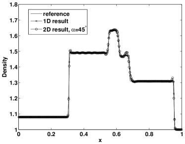
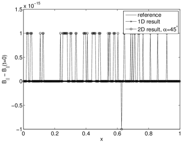
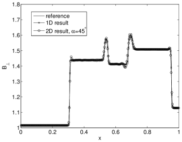
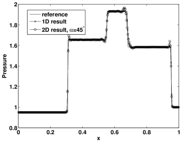
Figure 1: Plots of density, magnetic components in parallel and vertical direction along the normal of the shock front, and pressure of the 2.5D shock-tube problem. The reference solution is calculated with 1D grid and 1600 grid cells. The 1D and 2D results are calculated with 256 and 256$\times$256 cells respectively. Output is at $t$=0.1 for the reference solution and 1D result, and at $t=0.1/\sqrt{2}$ for 2D results with shock angle of $\alpha=45^{\circ}$. The parallel component of the magnetic fields ($B_{\parallel}$) is conserved with an accuracy of machine round-off errors.

4.2 One-dimensional MHD Caustics

This example is taken from Ryu et al. (1993). It was proposed as a test for hydro cosmology code to handle the thermal energy correctly. The formation of 1D caustics has been calculated from the initial sinusoidal velocity field along the x-direction with the peak value $1/2\pi$. The initial density and pressure has been set to be uniform with $\rho=1$ and $p=10^{-10}$. Hence the initial peak velocity corresponds to a Mach number of 1.2$\times$$10^{4}$. In the simulations, the pressure can easily become negative for this type of high Mach flow.

We test this problem with and without magnetic fields. If the magnetic fields are present, we set $B_{x}=B_{z}=0$, and only $B_{y}$ is nonzero. Different values of $B_{y}$ are tested. Fig. 2 shows the results at $t=3$ with 1024 cells. For this problem, the total energy version of the code will give a wrong pressure floor value, which is not shown here. The results shown in Fig. 2 are calculated using the combination of the total energy version with a modified entropy equation. It is clear that the strong magnetic fields ($B$=0.05) can suppress the density peak, while relatively weak magnetic fields ($B$=1E-3) have little impact on the density and pressure profile.

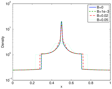
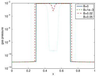
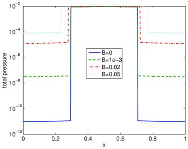
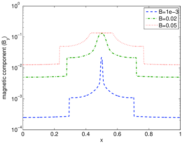
Figure 2: Plots of density, gas pressure, total pressure, and magnetic component ($B_{y}$) of 1D MHD caustics test at $t=3$. The modified entropy equation is solved.

We also solve the internal energy equation to follow the adiabatic changes correctly in the pre-shock region. Figure 3 shows the comparison between the modified entropy version and the internal energy version for $B_{y}=0.05$ case. The results are almost identical. Figure 3 also shows the comparison with different Riemann solvers. Apparently the HLL solver is very diffusive in the post-shock region so that it cannot recover the gas pressure correctly in the middle region.

Figure 3: Comparison of different approaches (left) and Riemann solvers (right) with the plots of gas pressure of 1D MHD caustics test at $t=3$. Initial $B_{y}=0.05$.

4.3 One-dimensional Cosmological Pancake Collapse

This example is also taken from Ryu et al. (1993). We set up the problem as a 1D pancake (i.e., the Zel’dovich pancake problem) in a purely baryonic Universe with $\Omega=1$ and $h=0.5$ in the comoving coordinates. The MHD solver with self-gravity module is tested. Initially, at $a_{i}=1$, which corresponds to $z_{i}=20$ in this test, a sinusoidal velocity field with the peak value $0.65/(1+z_{i})$ in the normalized units has been imposed in a box with the comoving size $64h^{-1}$Mpc. The baryonic density and pressure have been set to be uniform with $(\rho,p)=(1,6.2\times 10^{-8})$ in the normalized units. The calculation has been done with a different number of cells, with and without magnetic fields. When the magnetic fields are present, we use only the $B_{y}$ component, and set $B_{x}=B_{z}=0$.

Figure 4 shows the results with $B_{y}=0$, i.e., without the magnetic fields. The results for both the modified entropy version and internal energy version are shown. For comparison, we also show the results of TVD-ES code (Ryu et al. (1993)), running with the mass-diffusive correction.

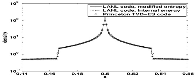
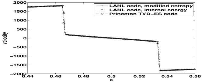
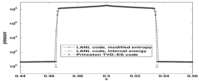
Figure 4: One-dimensional gravitational collapse of a pancake in the comoving coordinates with different codes. The number of cells is 1024. No magnetic fields are applied ($B=0$).

Figure 5 shows the results with magnetic fields. Different magnetic fields have different impact on the shock location and the peaks of density and magnetic fields. With a small $B_{y}=1.3e-6$, the magnetic fields have little impact on the shock and the density profile. The magnetic fields collapse in the same way as the density field does. As we increase the magnitude of the magnetic fields, the density peak in the post-shock region and shock location show large changes, while the profile in the pre-shock region has little change.

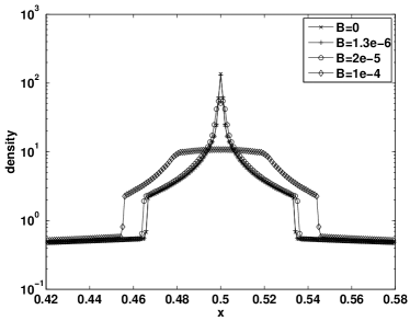
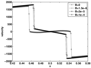
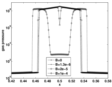
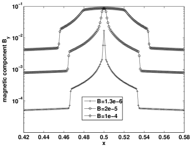
Figure 5: One-dimensional gravitational collapse of a pancake in the comoving coordinates with different magnitude of magnetic fields. The number of cells is 1024.

Figure 6 shows the comparison for different Riemann solvers applied to the modified entropy equation. The results for HLLC and the more sophisticated Roe’s solver are almost identical, while the result for HLL solver is not so good at the post-shock region.

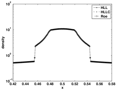
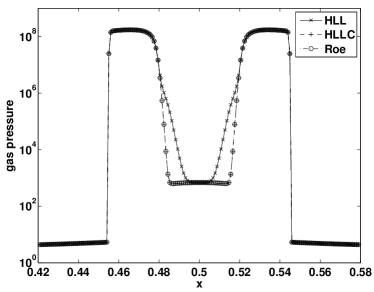
Figure 6: One-dimensional gravitational collapse of a pancake in the comoving coordinates with different Riemann solvers. The number of cells is 1024. $B_{y}=10^{-4}$.

4.4 Comparison with Other Codes for 3D Adiabatic CDM Universe

We have carried out a comparison of our cosmological MHD code with the original TVD-ES code of Ryu et al. (1993). We computed the adiabatic evolution of a purely baryonic Universe but with an initial CDM power spectrum with the following parameters: $\Omega=\Omega_{b}=1,~{}h=0.5,$, $n=1$ and $\sigma_{8}=1$, and the size of the computational cube is $L=64h^{-1}{\rm Mpc}$. We use the Bardeen et al. (1986) transfer function to calculate the power spectrum of the initial density fluctuations. This test problem is identical to that of Kang et al. (1994) except that the random numbers used to generate the initial condition are different. The Universe is evolved from $z=30$ to $z=0$. We use $256^{3}$ cells for each simulation performed. The comparisons are made at the final epoch, $z=0$.

Figure 7 shows a comparison of a mass-weighted histogram of the baryonic temperature at $z=0$ without magnetic fields between the original TVD-ES code and CosmoMHD. The mass-weighted histogram is calculated by using the temperature as $x$-axis and total mass in each temperature bin as the $y$-axis. They are in a good agreeement.

We have also performed another run with initial magnetic fields, $B_{x}=B_{z}=0$, $B_{y}$=2.5E-9 Gauss (which corresponds to 4.3176E-7 in code unit). Figure 8 shows a slice of the density and magnetic energy at $z=0$. We see that the distributions of density and magnetic field are strongly correlated, as expected. To demonstrate the impact of the CT method, we set the initial $B_{y}$=1E-5 Gauss, which corresponds to 0.0017 in code unit. Figure 9 shows the comparison of the divergence of the magnetic fields, averaged over the entire box, as a function of redshift. It is clear that without the CT method, the divergence of the magnetic fields grows in tandem with the growth of the magnetic field strength, and simulation results would hardly be meaningful. Since single-precision is used in our whole simulation, the divergence from the CT method is close to the round-off error. The temperature plots are shown in Fig. 10. The plasma beta becomes very small ($10^{-6}$) in many regions with these large magnetic fields. The dual-formulation must be used to track the internal energy accurately.

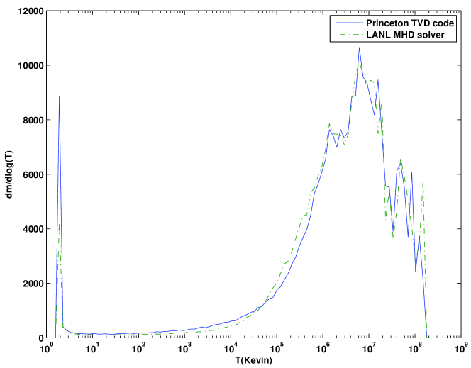
Figure 7: Mass-weighted temperature histogram at present (redshift z=0) for the 3D simulations of a purely baryonic adiabatic Universe.

Figure 8: Density and magnetic energy at present for the 3D simulations of a purely baryonic adiabatic Universe. Left: log density plot at z=0.5 slice. Right: log magnetic energy plot at z=0.5 slice. Initial magnetic fields are $B_{x}=B_{z}=0$ and $B_{y}$=4.3176E-7.

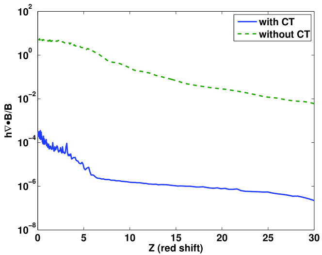
Figure 9: The scaled divergence ($h\nabla\cdot{\bf B}/B$) of the magnetic fields with and without constraint transport (CT) for the three-dimensional simulations of a purely baryonic adiabatic Universe during the whole time history. The initial $B_{y}$ at $Z=30$ is 0.0017.

Figure 10: Temperature plots of a slice at present for the 3D simulations of a purely baryonic adiabatic Universe. Left: log temperature plot without using CT at z=0.5 slice. Right: log temperature plot with CT at z=0.5 slice. Initial magnetic fields are $B_{x}=B_{z}=0$ and $B_{y}$=0.0017.

5 Discussion and Conclusions

We have developed and tested a modern cosmological MHD code (CosmoMHD). In the CosmoMHD code, five sets of equations are evolved simultaneously: (1) the ideal MHD equations for magneto-gasdynamics, (2) rate equations for multiple species of different ionizational states (including hydrogen, helium and oxygen), (3) the Vlasov equation for dynamics of collisionless particles (including dark matter particles and stellar particles), (4) the Poisson’s equation for obtaining the gravitational potential field and (5) the equation governing the evolution of the intergalactic ionizing radiation field, all in cosmological comoving coordinates. The MHD solver consists of several high-resolution schemes with finite-volume and finite-difference methods. The divergence-free condition of the magnetic field is preserved to an accuracy due just to round-off errors. Additional implemented physical processes include: (1) detailed cooling and heating processes due to all the principal line and continuum processes for a plasma of primordial composition as well as cooling and heating due to metals, (2) star formation processes and feedback processes from star formation including UV radiation and galactic superwinds, and (3) formation of supermassive black holes and associated feedback processes including radio jets/lobes.

The CosmoMHD code developed here may be applied to a variety of astrophysical/cosmological problems with or without self-gravity. We intend to study the formation and evolution of galaxies, clusters of galaxies and the intergalactic medium using this accurate code. Most importantly, we would like to investigate the role played by the AGN feedback in the form of powerful radio jets/lobes in regulating structure formation on scales from the cores of clusters of galaxies ($\sim 10$kpc) through giant lobes ($\sim 100$kpc$-1$Mpc) to large scales ($>1$Mpc). It seems prudent to check if many fundamental cosmological applications, such as weak gravitational lensing, formation and evolution of X-ray/SZ clusters and matter power spectrum with baryonic oscillation features, may be affected by this feedback effect. A thorough understanding of AGN feedback may be necessary to reduce systematic errors to levels that are commensurate with statistical errors that many of these important observations are expected to be able to achieve.

References

- Allen (2000) Allen, S.W. 2000, MNRAS, 315, 269
- Bahcall et al. (1999) Bahcall, N.A., Ostriker, J.P., Perlmutter, S., & Steinhardt, P. 1999, Science, 284, 1481
- (3) Balsara, D.S., & Spicer, D.S. 1999, J. Comput. Phys., 148, 133
- (4) D.S. Balsara and J.S. Kim, ApJ, 602 (2004) 1079.
- Bardeen et al. (1986) Bardeen, J.M., Bond, J.R., Kaiser, N., Szalay, A.S. ApJ, 304 (1986), 15
- Begelman (2004) Begelman, M.C. 2004, Coevolution of Black Holes and Galaxies, ed. L.C. Ho (Cambridge University Press), p374
- Binney (2000) Binney, J. 2000, in Gas and Galaxy Evolution, ASP conf. series, ed. Hibbard, Rupen, & van Gorkom Binney, J. 2004, in The Riddle of Cooling Flows in Galaxies and Clusters of Galaxies, eds. T. Reiprich, J. Kempner, and N. Soker
- Brio & Wu (1988) Brio, M., & Wu, C.C. 1988, J. Comput. Phys., 75, 400
- Bruggen & Kaiser (2001) Bruggen, M, & Kaiser, C.R. 2001, MNRAS, 325, 676
- Bruzual & Charlot (1993) Bruzual, A. G. & Charlot, S. 1993, ApJ, 405, 538
- Bruzual (2000) Bruzual, A. G. 2000, preprint (astro-ph/0011094)
- Bryan et al. (1995) Bryan, G.L., Norman, M.L., Stone, J.M., Cen, R., & Ostriker, J.P. 1995, Comp. Phys. Comm., 89, 149
- Carilli & Taylor (2002) Carilli, C.L., & Taylor, G.B. 2002, ARAA, 40, 319
- Cen (1992) Cen, R. 1992, ApJS, 78, 341
- Cen et al. (1995) Cen, R., Kang, H., Ostriker, J.P., & Ryu, D. 1995, ApJ, 451, 436
- Cen & Ostriker (1992) Cen, R., & Ostriker, J.P. 1992, ApJ, 399, L113
- Cen & Ostriker (1993) Cen, R., & Ostriker, J.P. 1993, ApJ, 417, 415
- Churazov et al. (2001) Churazov, E., Bruggen, M., Kaiser, C.R., Bohringer, H., & Forman, W. 2001, ApJ, 554, 261
- Cowie & Binney (1977) Cowie, L.L., & Binney, J. 1977, ApJ, 215, 723
- Croton et al. (2006) Croton, D.J., et al. 2006, MNRAS, 365, 11
- Dalla Vecchia et al. (2004) Dalla Vecchia, C., Bower, R.G., Theuns, T., Balogh, M.L., Mazzotta, P., & Frenk, C.S. 2004, MNRAS, 355, 995
- Deharveng et al. (2001) Deharveng, J.-M., Buat, V., Le Brun, B., Milliard, B., Kynth, D., Shull, J. M., & Gry, C. 2001, A&A, 375, 805
- Dolag et al. (1999) Dolag, K. et al. 1999, A&A, 348, 351
- Dolag et al. (2002) Dolag, K. et al. 2002, A&A, 387, 383
- Dolag et al. (2005) Dolag, K. et al. 2005, JCAP, 1, 9
- Einfeldt (1988) Einfeldt, B. 1988, SIAM J. Numer. Anal., 25, 294.
- Einfeldt et al. (1991) Einfeldt, B., Munz, C.D., Roe, P.L., & Sjogreen, B. 1991, J. Comput. Phys., 92, 273.
- Eggen, Lynden-Bell & Sandage (1962) Eggen, O.J., Lynden-Bell, D., & Sandage, A.R. 1962, ApJ, 136, 748
- Fabian (1994) Fabian, A.C. 1994, ARAA, 32, 277
- Fabian & Nulsen (1977) Fabian, A.C., & Nulsen, P.E.J. 1977, MNRAS, 180, 479
- Ferrarese & Merritt (2000) Ferrarese, L., & Merritt, D. 2000, ApJ, 539, L9
- Furlanetto & Loeb (2001) Furlanetto, S.R., & Loeb, A. 2001, ApJ, 556, 619
- Gebhardt et al. (2000) Gebhardt, K., et al. 2000, ApJ, 539, L13
- Gnedin & Ostriker (1997) Gnedin, N.Y., & Ostriker, J.P. 1997, 486, 581
- Harten, Lax, & van Leer (1983) Harten, A., Lax, P.D., & van Leer, B. 1983, SIAM Rev., 25, 35.
- Heckman et al. (2001) Heckman, T. M., Sembach, K. R., Meurer, G. R., Leitherer, C., Calzetti, D., & Martin, C. L. 2001, ApJ, 558, 56
- Henrik et al. (2004) Henrik, O., Binney, J., Bryan, G., & Slyz, A. 2004, MNRAS, 348, 1105
- (38) Hopkins, P.F., Hernquist, L., Cox, T.J., Di Matteo, T., Robertson, B., & Springel, V. 2005a, ApJ, 625, L71
- (39) Hopkins, P.F., Hernquist, L., Cox, T.J., Di Matteo, T., Robertson, B., & Springel, V. 2005b, ApJ, 630, 705
- (40) Hopkins, P.F., Hernquist, L., Cox, T.J., Di Matteo, T., Robertson, B., & Springel, V. 2005c, ApJ, 630, 716
- (41) Hopkins, P.F., Hernquist, L., Cox, T.J., Di Matteo, T., Robertson, B., & Springel, V. 2005d, ApJ, 632, 81
- Hopkins et al. (2006) Hopkins, P.F., Hernquist, L., Cox, T.J., Di Matteo, T., Robertson, B., & Springel, V. 2006, ApJS, 163, 1
- Hurwitz et al. (1997) Hurwitz, M., Jelinsky, P., & Dixon, W. V. D. 1997, ApJ, 481, L31
- Kaastra et al. (2004) Kaastra, J.S., et al. 2004, A&A, 413, 415
- Katz, Hernquist, & Weinberg (1992) Katz, N., Hernquist, L., & Weinberg, D.H 1992, ApJ, 399, L109
- Katz, Hernquist, & Weinberg (1996) Katz, N., Hernquist, L., & Weinberg, D.H 1996, ApJS, 105, 19
- Krauss & Turner (1995) Krauss, L., & Turner, M.S. 1995, Gen. Rel. Grav., 27, 1137
- Kronberg et al. (2001) Kronberg, P.P., Dufton, Q.W., Li, H., & Colgate, S.A. 2001, ApJ, 560, 178
- Levy et al. (2000) Levy, D., Puppo, G., & Russo, G. 2000, Appl. Numer. Math., 33, 407
- Levine & Gnedin (2006) Levine, R., & Gnedin, N.Y. 2006, ApJ, 649, L57
- Levy et al. (2002) Levy, D., Puppo, G., & Russo, G. 2002, preprint.
- Li (2005) Li, S. 2005, J. Comput. Phys., 203, 344
- Li & Li (2003) Li, S. & Li, H. 2003, Technical Report, Los Alamos National Laboratory
- Li et al. (2006) Li, H. et al. 2006, ApJ, 643, 92
- Magorrian et al. (1998) Magorrian, J., et al. 1998, AJ, 115, 2285
- Nakamura, et al. (2006) Nakamura, M., Li, H., & Li, S. 2006, ApJ, 652, 1059
- Omma & Binney (2004) Omma, H., & Binney, J. 2004, MNRAS, 350, L13
- Ostriker & Steinhardt (1995) Ostriker, J.P., & Steinhardt, P. 1995, Nature, 377, 600
- Ostriker, Bode,& Babul (2005) Ostriker, J.P., Bode, P., & Babul, A. 2005, ApJ, 634, 964
- Peres et al. (1998) Peres, C.B., Fabian, A.C., Edge, A.C., Allen, S.W., Johnstone, R.M., & White, D.A 1998, MNRAS, 298, 416.
- Peterson et al. (2003) Peterson, J.R., et al. 2003, ApJ, 590, 207
- Pettini et al. (2002) Pettini, M., Rix, S. A., Steidel, C. C., Adelberger, K. L., Hunt, M. P., & Shapley, A. E. 2002, ApJ, 569, 742
- Ponman, Cannon, & Navarro (1999) Ponman, T.J., Cannon, D.B., & Navarro, J.F. 1999, Nature, 397, 135
- Powell et al. (1999) Powell, K.G., Roe, P.L., Linde, T.J., Gombosi, T.I., & DeZeeuw, D.L. 1999, J. Comt. Phys., 154, 284
- Quilis et al. (2001) Quilis, V., Bower, R.G., & Balogh, M. 2001, MNRAS, 328, 1091
- Refregier (2003) Refregier, A. 2003, ARAA, 41, 645
- Richstone et al. (1998) Richstone, D., et al. 1998, Nature, 395, A14
- Robertson et al. (2006) Robertson, B., Hernquist, L., Cox, T.J., Di Matteo, T., Hopkins, P.F., Martini, P., & Springel, V. 2006, ApJ, 641, 90
- Roe & Balsara (1996) P. L. Roe and D. S. Balsara, SIAM J. Appl. Math., 56 (1996) 57-67.
- Ryu et al. (1993) Ryu, D., Ostriker, J.P., Kang, H., &, Cen, R. 1993, ApJ, 414, 1
- Ryu & Jones (1995) Ryu, D. & Jones, T.W. 1995, ApJ, 442, 228
- Ryu et al. (1998) Ryu, D. et al. 1998, A&A, 335, 19
- Ruszkowski, Bruggen, & Begelman (2004) Ruszkowski, M., Bruggen, M., & Begelman, M.C. 2004, ApJ, 615, 675
- Sajacki & Springel (2006) Sajacki, D., & Springel, V. 2006, ApJ, 366, 397
- Sazonov, Ostriker, & Sunyaev (2004) Sazonov, S. Y., Ostriker, J. P., & Sunyaev, R. A. 2004, MNRAS, 347, 144
- Scannapieco & Oh (2004) Scannapieco, E., & Oh, S.P. 2004, ApJ, 608, 62
- Silk & Rees (1998) Silk, J., & Rees, M.J. 1998, A&A, 331, L1
- Spergel et al. (2006) Spergel, D.N., et al. 2006, astro-ph/0603449
- Steinmetz (1996) Steinmetz, M. 1996, MNRAS, 278, 1005
- Stone & Norman (1992) Stone, J.M., & Norman, M.L. 1992, ApJS, 80, 791.
- Suginohara, & Ostriker (1998) Suginohara, T., & Ostriker, J.P. 1998, ApJ, 507, 16
- Toth (2000) Toth, G. 2000, J. Comt. Phys., 161, 605
- Tremaine et al. (2002) Tremaine, S., et al. 2002, ApJ, 574, 740
- Urry (2004) Urry, M. 2004, AGN Physics with the Sloan Digital Sky Survey, ed. G.T. Richards and P.B. Hall, ASP Conference Series, Volume 311 (San Francisco: Astronomical Society of the Pacific), p49
- van Leer (1974) van Leer, B. 1974, J. Comput. Phys., 14, 361
- White, Jones, Forman (1997) White, D.A., Jones, C., & Forman, W. 1997, MNRAS, 292, 419
- Woodward & Colella (1984) Woodward, P.R., & Colella, P. 1984, J. Comp. Phys., 54, 115
- Yoshida et al. (2002) Yoshida, N., Stoehr, F., Springel, V., & White, S.D.M. 2002, MNRAS, 335, 762
- Ziegler et al. (2006) Ziegler, E. 2006, AN, 327, 607