High-resolution imaging of the cosmic mass distribution from gravitational lensing of pregalactic HI

Abstract

Low-frequency radio observations of neutral hydrogen during and before the epoch of cosmic reionization will provide $\sim 1000$ quasi-independent source planes, each of precisely known redshift, if a resolution of $\sim 1$ arcminutes or better can be attained. These planes can be used to reconstruct the projected mass distribution of foreground material. Structure in these source planes is linear and gaussian at high redshift ($30<z<300$) but is nonlinear and nongaussian during re ionization. At both epochs, significant power is expected down to sub-arcsecond scales. We demonstrate that this structure can, in principle, be used to make mass images with a formal signal-to-noise per pixel exceeding 10, even for pixels as small as an arc-second. With an ideal telescope, both resolution and signal-to-noise can exceed those of even the most optimistic idealized mass maps from galaxy lensing by more than an order of magnitude. Individual dark halos similar in mass to that of the Milky Way could be imaged with high signal-to-noise out to $z\sim 10$. Even with a much less ambitious telescope, a wide-area survey of 21 cm lensing would provide very sensitive constraints on cosmological parameters, in particular on dark energy. These are up to 20 times tighter than the constraints obtainable from comparably sized, very deep surveys of galaxy lensing, although the best constraints come from combining data of the two types. Any radio telescope capable of mapping the 21cm brightness temperature with good frequency resolution ($\sim 0.05$ MHz) over a band of width $\lower 2.15277pt\hbox{$\;\buildrel>\over{\sim}\;$}10$ MHz should be able to make mass maps of high quality. The planned Square Kilometer Array (SKA) may be able to map the mass with moderate signal-to-noise down to arcminute scales, depending on the reionization history of the universe and the ability to subtract foreground sources.

1 introduction

Dark matter appears to be the dominant component of all structures larger than individual galaxies. In the standard paradigm its gravitational effects drive the linear growth and the subsequent nonlinear collapse of the fluctuations detected at $z\sim 1000$ in the cosmic microwave background (CMB). Our inability to “see” the dark matter, and so to image its distribution, has prevented a definitive observational verification of this paradigm. Simulations of structure formation predict all galaxies and galaxy clusters to sit within extended dark halos with regular and well-specified structural properties, but it has proved difficult to test these predictions convincingly. As first demonstrated by Kaiser & Squires (1993) the distortion of the images of distant objects caused by gravitational lensing can be used to reconstruct an image of the foreground mass distribution. All successful applications so far have used distant galaxies as the sources. The resolution and signal-to-noise of the resulting maps are fundamentally limited by the abundance and intrinsic ellipticity of these sources. Even with deep satellite data the effective density of usable galaxies does not exceed about 100 per sq.arcmin. For a map with 1 arcmin pixels this corresponds to a signal-to-noise per pixel (ratio of rms expected physical fluctuation to rms noise fluctuation) of about 0.75; for 10 arcmin pixels this ratio is about 2.5. As a result, only the centers of the most massive galaxy clusters can be detected at high signal-to-noise in galaxy-based mass maps. In this paper we show that much higher resolution and effective signal-to-noise can, in principle, be achieved by using high redshift neutral hydrogen as the source, rather than galaxies.

There has been a great deal of interest in the possibility of observing the hyperfine transition of hydrogen (the 21 cm line) from the intergalactic (or pregalactic) medium at high redshift (see Furlanetto, Oh & Briggs 2006, for an extensive review). There are two essentially disjoint epochs from which 21 cm radiation should be observable. At a redshift of $z\simeq 300$ neutral hydrogen (HI) became thermally decoupled from the CMB. The gas kinetic temperature then fell below the CMB temperature $T_{r}$ due to their different adiabatic cooling laws. For a while the spin temperature $T_{s}$ remained coupled to the kinetic temperature by atomic collisions, but at $z\sim 30$ the collision rate became so low that the spin temperature decoupled from the kinetic temperature and returned to equilibrium with the CMB. During the period $30<z<300$, $T_{s}$ was below $T_{r}$ and there was a net absorption of CMB photons through the 21 cm line. The observable quantity is the brightness temperature $T_{b}=(T_{s}-T_{r})(1-e^{\tau})\simeq(T_{s}-T_{r})\tau$ which depends on the optical depth, $\tau$, which is in turn proportional to the density of HI. A map of $T_{b}$ on the sky and in frequency would thus be a three dimensional map of the HI density, which is directly proportional to the mass density at these redshifts. The physics during this epoch of 21 cm absorption is simple, and predictions within the standard cosmogony are straightforward and robust.

The second epoch with observable 21 cm effects is considerably less well characterized. It is known that almost all intergalactic hydrogen at $z<6.5$ is ionized. It is believed that radiation from the first generation of stars and/or quasars caused this reionization between $z\sim 6.5$ and $z\sim 30$. The latest CMB constraints give $8.5<z_{reion}<22$ at 68% confidence (Spergel et al. 2006). A variety of mechanisms will transfer energy from X-ray and/or Lyman-$\alpha$ radiation to the HI gas during reionization, thereby raising $T_{s}$ above the CMB temperature and making the 21 cm line visible in emission. After reionization is complete, too little HI is left to be observable. The mean free path for X-rays through the neutral IGM at $z<15$ can exceed the Hubble length, so the spin temperature for much of the HI could have been raised uniformly before significant reionization occurred. Lyman-continuum radiation is expected to produce ionized bubbles that expand until they overlap. Reionization finally completes as the last interbubble clumps are evaporated. During this period, Ly-$\alpha$ radiation passes freely through ionized regions but is resonantly scattered in neutral regions, thereby raising their spin temperature and producing 21 cm emission. How rapid and inhomogeneous this process was is highly uncertain and is likely to remain so until it is directly measured. It is also possible that shock heating of HI gas during the collapse of pregalactic objects could raise $T_{s}$ enough for 21 cm emission to be visible before reionization begins (Kuhlen, Madau & Montgomery 2006).

Gravitational lensing distorts our image of the 21 cm emission and absorption by moving the angular positions of points on the sky while keeping the associated surface brightness (and thus brightness temperature) unchanged. For this reason a smooth background radiation field is unaffected by lensing. The observed map of brightness temperature thus reflects both the intrinsic structure of the fluctuations and the lensing distortions. To separate the two, we use the fact that in a given direction the intrinsic structure of maps at sufficiently separated frequencies (hence redshifts) will be statistically uncorrelated, while the foreground lensing distribution will be the same. Below we show how the maps can be combined so as to average out the intrinsic temperature fluctuations while preserving the lensing signal. In essence, the gradients of brightness temperature maps at a set of sufficiently well-spaced frequencies are independently and isotropically distributed in the absence of lensing, but display a coherence which is a direct measure of the lensing-induced shear when the foreground mass distribution is taken into account.

Gravitational lensing of pregalactic 21 cm signals has previously been considered by several authors. In particular, Zahn & Zaldarriaga (2006) extended to 3-dimensions (angle on the sky + redshift of source) the techniques developed by Hu (2001) for detecting lensing in the CMB, and they applied them to high-redshift 21 cm emission. In retrospect we find that the Fourier-space version of the method presented here is related to their method (see Appendices B and C for details) and that our method is related to one developed by Seljak & Zaldarriaga (1999) for detecting lensing in the CMB. Cooray (2004) had already discussed applying the original 2-dimensional Hu (2001) method to the 21 cm absorption epoch, but this misses the main advantage offered by the radio technique, namely the large number of available quasi-independent source planes. Finally, Pen (2004) discussed measuring gravitational lensing effects in the 21 cm emission by looking for anisotropic effects on the second order statistics of the brightness fluctuations. This does not estimate the gravitational shear directly by comparing maps at different frequencies in the same direction, and so is much less sensitive than the approaches suggested here and by Zahn & Zaldarriaga (2006).

The 21 cm emission/absorption has two major advantages over the CMB as a background source for lensing studies. Since lensing conserves surface brightness, it can only redistribute structure that already exists in the source. The CMB has very little structure on the angular scales where lensing is significant ($\lower 2.15277pt\hbox{$\;\buildrel<\over{\sim}\;$}1$ arcmin) so that lensing effects are very weak. The second advantage is that the CMB provides only one temperature field on the sky while the 21 cm emission/absorption provides many, all of which are lensed by the same foreground mass distribution. Although the CMB comes from higher redshift, this is a relatively minor advantage since most of the structure detected by lensing is at much smaller redshift than either source.

Our paper is organized as follows. In section 2 an estimator for the gravitational shear is derived and in section 3 the noise in that estimator is discussed and quantified using a particular model for correlations in the 21 cm brightness temperature. The expected lensing signal and the size of objects that could be detected are calculated in §4. The prospects for measuring cosmological parameters with 21 cm lensing are discussed in section 5. The observational prospects given currently planned telescope designs are discussed in §6. In the appendices several technical issues are addressed and alternative methods for measuring the lensing signal are described.

2 an estimator for the gravitational shear

The observed deviation in the brightness temperature of the 21 cm emission at a redshift $z$ (or equivalently frequency $\nu$) and a point on the sky, $\vec{\theta}$ will be denoted $T(\vec{\theta},\nu)$. We seek to construct a statistic from this temperature that, when summed over frequency bands, $\nu$, preserves the lensing signal while smoothing out the fluctuations in $T(\vec{\theta},\nu)$. A statistic will have these properties if it has the same properties when averaged over an ensemble of temperature fields at a fixed $\nu$ while keeping the lensing contribution fixed. All statistics that are first-order in $T(\vec{\theta},\nu)$ vanish with this averaging because of isotropy.

We will now show that it is possible to isolate the lensing contribution in the second order statistics of the gradient of the temperature field, $\vec{\nabla}T(\vec{\theta},\nu)$. The small angle, or “flat sky”, approximation will be used throughout this paper and is well justified for the angular scales that are considered. The observed temperature at a point on the sky, $\vec{\theta}$, is the source temperature at $\vec{\theta}^{\prime}=\vec{\theta}+\vec{\alpha}(\vec{\theta},\nu)$ plus noise, where $\vec{\theta}^{\prime}$ is the position on the source plane (what the position would be in the absence of lensing) and $\vec{\alpha}(\vec{\theta},\nu)$ is the position shift caused by lensing (hereafter the deflection). Thus the observed gradient of the temperature will be

$$\nabla_{k}T(\vec{\theta},\nu)=\left(\delta_{ki}+\alpha_{ki}(\vec{\theta},\nu)\right)\nabla^{\prime}_{i}{\mathcal{T}}(\vec{\theta}^{\prime},\nu)+N_{k}(\vec{\theta},\nu)~{}~{}~{},~{}~{}~{}\alpha_{ki}(\vec{\theta},\nu)\equiv\frac{\partial\alpha_{i}(\theta,\nu)}{\partial\theta_{k}}~{},$$ (1)

where ${\mathcal{T}}(\vec{\theta},\nu)$ is the real, unlensed brightness temperature and $\vec{N}(\vec{\theta},\nu)$ is the noise in the measured gradient. Repeated indices are summed over. The square of the magnitude of the observed gradient will be

$$|\nabla T(\vec{\theta})|^{2}=|\nabla^{\prime}{\mathcal{T}}(\vec{\theta}^{\prime})|^{2}+\left(2\alpha_{ij}(\vec{\theta})+\alpha_{ik}(\vec{\theta})\alpha_{jk}(\vec{\theta})\right)\nabla^{\prime}_{i}{\mathcal{T}}(\vec{\theta}^{\prime})\nabla^{\prime}_{j}{\mathcal{T}}(\vec{\theta}^{\prime})$$ (2)

$$+2\left(\delta_{ij}+\alpha_{ij}(\vec{\theta})\right)N_{i}(\vec{\theta})\nabla^{\prime}_{j}{\mathcal{T}}(\vec{\theta}^{\prime})+|\vec{N}(\vec{\theta})|^{2}.$$

where the $\nu$’s have been left out for brevity.

The source emission, the deflection and the noise will all be statistically independent so we can consider them separately. Averaging over the source gives

$$\left\langle\nabla^{\prime}_{i}{\mathcal{T}}(\vec{\theta}^{\prime},\nu)\right\rangle = 0~{},$$ (3)

$$\left\langle\nabla^{\prime}_{i}{\mathcal{T}}(\vec{\theta}^{\prime},\nu)\nabla^{\prime}_{j}{\mathcal{T}}(\vec{\theta}^{\prime},\nu)\right\rangle = \frac{1}{2}\delta_{ij}\sigma_{\nabla}^{2}(\nu)$$ (4)

where this defines $\sigma_{\nabla}^{2}(\nu)$ and $\delta_{ij}$ is the Kronecker delta.

The distortion matrix $\alpha_{ij}$ can be decomposed into quantities that are commonly used in lensing, the convergence $\kappa$, the shear $\gamma$ and a rotation parameter $\beta$,

$${\bf\alpha}=\left(\begin{array}[]{ccc}\kappa+\gamma_{1}&\gamma_{2}-\beta\\ \gamma_{2}+\beta&\kappa-\gamma_{1}\end{array}\right).$$ (5)

Using this decomposition we find $\alpha_{ik}(\vec{\theta},\nu)\alpha_{jk}(\vec{\theta},\nu)$ to correspond to the matrix

$$\left(\begin{array}[]{ccc}\kappa^{2}+\gamma^{2}+\beta^{2}+2(\gamma_{1}\kappa-\gamma_{2}\beta)&2(\gamma_{2}\kappa+\gamma_{1}\beta)\\ 2(\gamma_{2}\kappa+\gamma_{1}\beta)&\kappa^{2}+\gamma^{2}+\beta^{2}-2(\gamma_{1}\kappa-\gamma_{2}\beta)\end{array}\right).$$ (8)

The rotation term $\beta$ comes from coupling between different lens planes and is second order in the surface density. It is expected to be very small in nearly all cases so we will neglect it in what follows, although its inclusion would be straightforward. Because of isotropy and the requirement that the usual angular size distance be correct on average, we have $[\alpha_{ij}(\vec{\theta},\nu)]_{\Omega}=0$ where $[...]_{\Omega}$ denotes an average over direction on the sky, and

$$\sigma_{\kappa}^{2}(\nu)\equiv[\gamma^{2}(\nu)]_{\Omega}=[\kappa^{2}(\nu)]_{\Omega}\ ,$$ (9)

where $\gamma^{2}=\gamma_{1}^{2}+\gamma_{2}^{2}$. The second equality follows from the deflection field being a potential field (i.e. assuming $\beta=0$).

We now construct three second-order quantities from the observed temperature gradient,

$$\Gamma_{1}(\vec{\theta},\nu) \equiv \frac{1}{2}\left(\nabla_{1}T(\vec{\theta},\nu)\nabla_{1}T(\vec{\theta},\nu)-\nabla_{2}T(\vec{\theta},\nu)\nabla_{2}T(\vec{\theta},\nu)\right),$$ (10)

$$\Gamma_{2}(\vec{\theta},\nu) \equiv \nabla_{1}T(\vec{\theta},\nu)\nabla_{2}T(\vec{\theta},\nu),$$ (11)

and

$$\Gamma_{3}(\vec{\theta},\nu) \equiv \frac{1}{2}\left|\nabla T(\vec{\theta},\nu)\right|^{2},$$ (12)

where the indices on the gradient symbols refer to the two axes of the chosen orthogonal coordinate system. For a given direction (and hence deflection field) the averages of these are

$$\left\langle\Gamma_{1}(\vec{\theta},\nu)\right\rangle = \sigma_{\nabla}^{2}(\nu)\gamma_{1}(\vec{\theta},\nu)\left(1+\kappa(\vec{\theta},\nu)\right)+\frac{1}{2}\left(\left\langle N_{1}(\nu)N_{1}(\nu)\right\rangle-\left\langle N_{2}(\nu)N_{2}(\nu)\right\rangle\right)$$ (13)

$$\left\langle\Gamma_{2}(\vec{\theta},\nu)\right\rangle = \sigma_{\nabla}^{2}(\nu)\gamma_{2}(\vec{\theta},\nu)\left(1+\kappa(\vec{\theta},\nu)\right)+\left\langle N_{1}(\nu)N_{2}(\nu)\right\rangle$$ (14)

$$\left\langle\Gamma_{3}(\vec{\theta},\nu)\right\rangle = \frac{1}{2}\sigma_{\nabla}^{2}(\nu)\left(1+2\kappa(\vec{\theta},\nu)+\kappa(\vec{\theta},\nu)^{2}+\gamma(\vec{\theta},\nu)^{2}\right)+\frac{1}{2}\sigma_{N}^{2}(\nu),$$ (15)

where $\sigma_{N}^{2}(\nu)$ is the average of $|\vec{N}(\vec{\theta})|^{2}$ over random realizations of the noise. If the noise is isotropic it will drop out of both (13) and (14). This can be seen by expressing the noise vector in terms of its magnitude and polar angle and then requiring that the direction be random. However, in general the noise may not be isotropic so we retain these terms. To lowest order the first terms in the averages (13) and (14) are proportional to the gravitational shear and (15) is related to the convergence.

The lensing signal from a single redshift slice will be dominated by noise so we wish to add up frequency channels to reduce the noise. The convergence and shear are slowly varying functions of $\nu$ at the high redshifts we are considering, so for now we will assume $\gamma(\vec{\theta},\nu)$ to be independent of $\nu$ within the frequency band being used. This suggests estimating the shear at a point on the sky through

$$\tilde{\gamma}_{i}(\vec{\theta})=\sum^{\nu_{2}}_{\nu=\nu_{1}}\omega_{\nu}\left\{\Gamma_{i}(\vec{\theta},\nu)-\left[\Gamma_{i}(\vec{\theta},\nu)\right]_{\Omega}\right\}$$ (16)

where the sum is over frequency channels. The weights, $\omega_{\nu}$, are normalized so that the mean values are

$$\left\langle\tilde{\gamma}_{1,2}(\vec{\theta})\right\rangle=\gamma_{1,2}(\vec{\theta})\left(1+\kappa(\vec{\theta})\right)\simeq\gamma_{i}(\vec{\theta}),$$ (17)

and

$$\left\langle\tilde{\gamma}_{3}(\vec{\theta})\right\rangle=\kappa(\vec{\theta})+\frac{1}{2}(\kappa(\theta)^{2}+\gamma(\theta)^{2}-2\sigma^{2}_{\kappa})\simeq\kappa(\vec{\theta}).$$ (18)

The weights will be determined in the next section. Except along exceptional lines of sight (through the very centers of galaxies and galaxy clusters) $\kappa(\vec{\theta})$ is much smaller than one. As we show explicitly below, the variance $\sigma_{\kappa}^{2}$ is thus small, and (16) in effect provides an unbiased map of $\vec{\gamma}(\vec{\theta})$ all the way back to the beginning of structure formation. We will sometimes refer to $\tilde{\gamma}_{i}(\vec{\theta})$ as the shear estimators even though the 3rd component is an estimator for the convergence, and $\tilde{\gamma}_{3}(\vec{\theta})$ will sometimes be written as $\tilde{\kappa}(\vec{\theta})$.

3 noise levels

3.1 Instrumental, foreground and irreducible noise

There will be a number of sources of noise in the estimators (16). In particular, there will be noise from the instrumentation, from terrestrial interference, and from incomplete subtraction of galactic and extragalactic foreground emission. This noise is encapsulated in the $\vec{N}(\vec{\theta},\nu)$ vector field. We will refer to these sources of noise collectively as foreground noise. It is expected that foreground emission will be removed to high accuracy by using the fact that it varies slowly with frequency, whereas the 21 cm emission/absorption signal (and particularly the angular gradient of this signal) decorrelates for even small separations along the line-of-sight (see Zaldarriaga, Furlanetto & Hernquist 2004; Santos, Cooray, & Knox 2005). The removal process could, however, leave noise with correlations in both frequency and position on the sky. For currently planned generations of instruments, this residual is expected to be as small as or smaller than the purely instrumental or thermal noise. The lensing signal is also coherent in frequency, but foreground subtraction will not effect it because lensing is multiplicative while while the foregrounds are additive, see equation (1). Lensing does not cause correlations between frequency channels, it causes spatial correlations within a frequency channel that are the same as in the other channels.

In addition to foreground noise there is noise from the randomness of the $\nabla T(\vec{\theta},\nu)$ field itself. Clearly, this cannot be reduced by any improvement in technology or foreground subtraction, so we will refer to it as the irreducible noise. It depends only on the intrinsic correlations in the 21 cm signals and on the range of frequency, or redshift, over which the signals are mapped. We will find that for any telescope which is able to map the 21 cm signals, the total noise in the shear estimate will automatically be near the irreducible value. For this reason it is both a lower limit and a good benchmark.

We must also differentiate between the noise per pixel and the noise in the average $\tilde{\gamma}(\vec{\theta})$ over a patch of sky which is larger than the pixel size. By pixel we mean the smallest resolvable region of the sky as set by the telescope. If the angular correlations in the noise drop off more rapidly than the correlations in the shear, then the signal-to-noise ratio will be maximal on an angular scale that is larger than the pixel size. We will refer to a region of sky over which $\tilde{\gamma}(\vec{\theta})$ is averaged as a patch in the shear map. A patch could be a square region, a circular aperture, a gaussian smoothing window or any other localized window.

The variances in the magnitude of our shear estimators, (16), are given by

$$\sigma^{2}_{\tilde{\gamma}}(\delta\Theta) = \int\int d^{2}\theta d^{2}\theta^{\prime}W(\vec{\theta};\delta\Theta)W(\vec{\theta^{\prime}};\delta\Theta)\sum_{\nu}\sum_{\nu^{\prime}}~{}\omega_{\nu}\omega_{\nu^{\prime}}\sum_{i=1}^{2}\left\langle\Gamma_{i}(\nu,\vec{\theta})\Gamma_{i}(\nu^{\prime},\vec{\theta}^{\prime})\right\rangle~{},$$ (19)

$$\sigma^{2}_{\tilde{\kappa}}(\delta\Theta) = \sigma^{2}_{\tilde{\gamma}_{3}}(\delta\Theta)$$ (20)

$$= \int\int d^{2}\theta d^{2}\theta^{\prime}W(\vec{\theta};\delta\Theta)W(\vec{\theta^{\prime}};\delta\Theta)\sum_{\nu}\sum_{\nu^{\prime}}~{}\omega_{\nu}\omega_{\nu^{\prime}}\left[\left\langle\Gamma_{3}(\nu,\vec{\theta})\Gamma_{3}(\nu^{\prime},\vec{\theta}^{\prime})\right\rangle-\left\langle\Gamma_{3}(\nu)\right\rangle\left\langle\Gamma_{3}(\nu^{\prime})\right\rangle\right]~{},$$ (21)

where $W(\vec{\theta};\delta\Theta)$ is the window function defining the patch (normalized to one when integrated over $\vec{\theta}$) and $\delta\Theta$ is its characteristic angular scale. The noise in the magnitude of the shear per pixel (i.e. in the original unsmoothed detection) is $\sigma^{2}_{\tilde{\gamma}}(0)$ while the noise in the isotropic estimator is $\sigma^{2}_{\tilde{\gamma}_{3}}(\delta\Theta)$. Note that the tildes are used to differentiate between noise in the estimator, $\sigma_{\tilde{\gamma}}$ and the variance in the signal, $\sigma_{\gamma}$. With some assumptions the correlation functions can be simplified

$$\sum_{i=1}^{2}\left\langle\Gamma_{i}(\nu,\vec{\theta})\Gamma_{i}(\nu^{\prime},\vec{\theta}^{\prime})\right\rangle = 2\,\left\langle\Gamma_{2}(\nu,\vec{\theta})\Gamma_{2}(\nu^{\prime},\vec{\theta}^{\prime})\right\rangle\$$ (22)

$$= 2\left\langle\nabla_{1}T(\nu,\vec{\theta})\nabla_{2}T(\nu,\vec{\theta})\nabla_{1}T(\nu^{\prime},\vec{\theta}^{\prime})\nabla_{2}T(\nu^{\prime},\vec{\theta}^{\prime})\right\rangle$$ (23)

$$= 2\left\langle\nabla_{1}T(\nu,,\vec{\theta})\nabla_{1}T(\nu^{\prime},\vec{\theta}^{\prime})\right\rangle^{2},$$ (24)

and

$$\left\langle\Gamma_{3}(\nu,\vec{\theta})\Gamma_{3}(\nu^{\prime},\vec{\theta}^{\prime})\right\rangle-\left\langle\Gamma_{3}(\nu)\right\rangle\left\langle\Gamma_{3}(\nu^{\prime})\right\rangle=\left\langle\nabla_{1}T(\nu,\vec{\theta})\nabla_{1}T(\nu^{\prime},\vec{\theta}^{\prime})\right\rangle^{2}.$$ (25)

In (22) we used the fact that rotational invariance requires that the noise in both components of $\gamma(\vec{\theta})$ be the same, so we choose to find the variance in the simpler $\Gamma_{2}(\nu)$ and double it to account for the other component. To get from (23) to (24) we have assumed that each component of $\nabla T(\nu)$ is normally distributed so that the fourth moment can be reduced to second moments. In addition, we assume that the temperature field is isotropic so that there is no cross-correlation between the components. The same assumptions are used in expression (25).

Replacing the observed gradient in (24) with the true temperature gradient plus noise gives the result

$$\sigma^{2}_{\tilde{\gamma}}(\delta\Theta) = 2\sigma^{2}_{\tilde{\kappa}}(\delta\Theta)~{}~{}~{}~{}~{}~{}~{}~{}~{}~{}~{}~{}~{}~{}~{}~{}~{}~{}~{}~{}~{}~{}~{}~{}~{}~{}~{}~{}~{}~{}~{}~{}~{}~{}~{}~{}~{}~{}$$ (26)

$$= \frac{1}{2}\sum_{\nu}\sum_{\nu^{\prime}}~{}\omega_{\nu}\omega_{\nu^{\prime}}{\mathcal{A}}(\nu,\nu^{\prime},\delta\Theta)~{},$$ (27)

where

$${\mathcal{A}}(\nu,\nu^{\prime},\delta\Theta)\equiv\int d^{2}\theta~{}\overline{W}(\vec{\theta};\delta\Theta)\left[\xi_{\nabla}(\nu,\nu^{\prime},\theta)+\xi_{N}(\nu,\nu^{\prime},\theta)\right]^{2},$$ (28)

$$\overline{W}(\vec{\theta};\delta\Theta)=\int d^{2}\theta^{\prime}~{}W(\vec{\theta}^{\prime}+\vec{\theta}/2;\delta\Theta)W(\vec{\theta}^{\prime}-\vec{\theta}/2;\delta\Theta),$$ (29)

and

$$\xi_{\nabla}(\nu,\nu^{\prime},\theta=|\vec{\theta}^{\prime}-\vec{\theta}^{\prime\prime}|)\equiv\sum_{i=1}^{2}\left\langle\nabla_{i}{\mathcal{T}}(\nu,\vec{\theta}^{\prime})\nabla_{i}{\mathcal{T}}(\nu^{\prime},\vec{\theta}^{\prime\prime})\right\rangle~{}~{}~{}~{}~{}{\rm implying}~{}~{}~{}~{}~{}\sigma^{2}_{\nabla}(\nu)=\xi_{\nabla}(\nu,\nu,0),$$ (30)

The correlation function $\xi_{N}(\nu,\nu^{\prime},\theta)$ is similarly defined. The pixel and frequency response functions are included in ${\mathcal{T}}(\vec{\theta})$.

The optimal weights, $\omega_{\nu}$, can be calculated numerically, but a very good analytic approximation can be found by assuming that they vary slowly over the frequency range in which ${\mathcal{T}}(\nu)$ is correlated (${\mathcal{A}}(\nu,\nu^{\prime})\simeq{\mathcal{A}}(\nu,\nu)$). In this case $\omega_{\nu^{\prime}}\simeq\omega_{\nu}$ in (27). Minimizing this subject to the constraint (17) gives the weights

$$\omega_{\nu}=\frac{\sigma^{2}_{\nabla}(\nu)}{\sum_{\nu^{\prime}}{\mathcal{A}}(\nu,\nu^{\prime})}\left(\sum_{\nu^{\prime}}\frac{\left(\sigma^{2}_{\nabla}(\nu^{\prime})\right)^{2}}{\sum_{\nu^{\prime\prime}}{\mathcal{A}}(\nu^{\prime},\nu^{\prime\prime})}\right)^{-1}.$$ (31)

Substituting this back into (27) gives the noise

$$\sigma^{2}_{\tilde{\gamma}}(\delta\Theta)=\frac{1}{2}\left(\sum_{\nu}\frac{\left(\sigma^{2}_{\nabla}(\nu)\right)^{2}}{\sum_{\nu^{\prime}}{\mathcal{A}}(\nu,\nu^{\prime})}\right)^{-1}.$$ (32)

If the noise in the brightness temperature map is small compared to the fluctuations in the temperature itself, $\xi_{N}(\nu,\theta)<\xi_{\nabla}(\nu,\theta)$, which is a minimal requirement for mapping the brightness temperature, then the foreground noise will drop out of (28) and the irreducible noise limit will be reached. To approach this noise level it is not necessary to eliminate all foreground noise. Thus a telescope designed to map the brightness temperature will naturally achieve a noise level in $\tilde{\gamma}(\vec{\theta})$ that is close to the irreducible value. The correlations in frequency might be set by the bandwidth or by the intrinsic correlations in the brightness temperature.

It is often convenient to express the lensing noise (32) in terms of the (cross-)power spectra of the brightness temperature $\overline{C}^{T}_{\ell}(\nu,\nu^{\prime})$ and the noise in the temperature $\overline{C}^{N}_{\ell}(\nu,\nu^{\prime})$. This can be done by Fourier transforming the temperature and gives

$${\mathcal{A}}(\nu,\nu^{\prime},\delta\Theta)=\int\frac{d^{2}L}{(2\pi)^{2}}~{}|\tilde{W}(L,\delta\Theta)|^{2}\int\frac{d^{2}\ell}{(2\pi)^{2}}~{}|\ell|^{2}|\vec{\ell}-\vec{L}|^{2}\left(\overline{C}^{T}_{\ell}(\nu,\nu^{\prime})+\overline{C}^{N}_{\ell}(\nu,\nu^{\prime})\right)\left(\overline{C}^{T}_{|\ell+L|}(\nu,\nu^{\prime})+\overline{C}^{N}_{|\ell+L|}(\nu,\nu^{\prime})\right)$$ (33)

and

$$\sigma^{2}_{\nabla}(\nu)=\int\frac{d^{2}\ell}{(2\pi)^{2}}~{}|\ell|^{2}\overline{C}^{T}_{\ell}(\nu,\nu).$$ (34)

For a further discussion of calculating things in Fourier-space see appendices B and C.

To determine the possible capabilities of 21 cm lensing experiments we now investigate the optimal case in which the irreducible limit is reached with a bandwidth that is much smaller than the intrinsic correlation length of the temperature. In the limit of infinitely narrow bandwidths the sums in eq. (32) can be converted into integrals. The function ${\mathcal{A}}(\nu,\nu^{\prime},\vec{\theta})$ defines a volume in frequency and angle within which the structure or noise is too strongly correlated to contribute “independent” information to the shear measurement. A very useful approximation to this volume can be found by calculating its characteristic length in frequency at $\theta=0$ and its characteristic angular area at $\nu^{\prime}=\nu$. For the temperature gradient alone these are

$$\Delta\nu_{\nabla}(\nu)\equiv\int_{0}^{\infty}d\nu^{\prime}~{}\left(\frac{\xi_{\nabla}(\nu,\nu^{\prime},0)}{\sigma^{2}_{\nabla}(\nu)}\right)^{2}$$ (35)

and

$$\Delta\Omega_{\nabla}(\nu)\equiv\int d^{2}\theta~{}\left(\frac{\xi_{\nabla}(\nu,\nu,\theta)}{\sigma^{2}_{\nabla}(\nu)}\right)^{2}.$$ (36)

Analogous correlation lengths can be defined for the noise term and for the cross-term. Note that these correlation lengths are defined with the correlation function squared, temperature to the fourth power, which makes them significantly smaller than the usual correlation lengths defined with the first power of the correlation function.

When the patch size is near $\Delta\Omega_{\nabla}(\nu)$ there will be only a few quasi-independent areas per patch. To account for this it is convenient to define the quantity

$${\mathcal{N}}_{\nabla}(\nu;\delta\Theta)\equiv\int d^{2}\theta~{}\left(\frac{\xi_{\nabla}(\nu,\nu,\theta)}{\sigma^{2}_{\nabla}(\nu)}\right)^{2}\overline{W}(\vec{\theta};\delta\Theta).$$ (37)

This quantity is essentially the area of a correlated region divided by the area of the patch. Two limiting cases are instructive. For a very small patch ${\mathcal{N}}_{\nabla}(\nu;\delta\Theta)\rightarrow 1$ and for a patch much larger than the intrinsic correlation length ${\mathcal{N}}_{\nabla}(\nu;\delta\Theta)\rightarrow\overline{W}(0;\delta\Theta)\Delta\Omega_{\nabla}(\nu)$ ($=\Delta\Omega_{\nabla}(\nu)/(4\pi\delta\Theta^{2})$ for a Gaussian patch). One would like the data to be collected in frequency channels with a width smaller than $\Delta\nu_{\nabla}(\nu)$, otherwise the irreducible noise will be increased. Instrumental design or foreground noise actually result in there being an optimal bandwidth that is near $\Delta\nu_{\nabla}(\nu)$ as will be shown in section 6.

Using the above definitions in (32) a simple approximation for the irreducible noise is found,

$$\sigma^{2}_{\tilde{\gamma}}(\delta\Theta)\simeq\frac{1}{2}\left(\int^{\nu_{2}}_{\nu_{1}}d\nu~{}\frac{1}{\Delta\nu_{\nabla}(\nu){\mathcal{N}}_{\nabla}(\nu,\delta\Theta)}\right)^{-1}.$$ (38)

When the patch size is very close to the pixel size the complete integrals in (28) must be carried out to obtain an accurate result, but for the purposes of this section this is not necessary. The limit for small $\delta\Theta$ is the noise per pixel. It is easy to see from (38) and (37) that the square of the irreducible noise is essentially one over twice the number of correlated volumes in a patch.

The above estimates assume that $\sigma^{2}_{\nabla}(\nu)$, the variance in the intrinsic temperature within a frequency channel, can be measured exactly so that the estimators $\tilde{\gamma}_{i}$ can be normalized properly. This is normally a good approximation as we now show. The variance in the gradient can be found by averaging over position on the sky in the entire surveyed region. Using (2) and dropping all terms higher than second order in $\kappa$ and $\gamma$ results in

$$\sigma^{2}_{K} \equiv \left\langle\left[\left(|\nabla T(\nu)|^{2}\right)^{2}\right]_{\Omega}\right\rangle$$ (39)

$$= 2\sum_{\nu}\sum_{\nu^{\prime}}~{}\omega_{\nu}\omega_{\nu^{\prime}}\int_{\Omega}d^{2}\theta\left\{\xi_{\nabla}(\nu,\nu^{\prime},\theta)^{2}\left(1+2\sigma_{\kappa}^{2}+2\xi_{\kappa}(\theta)\right)\right.$$ (42)

$$+2\xi_{\nabla}(\nu,\nu^{\prime},\theta)\xi_{N}(\nu,\nu^{\prime},\theta)\left(1+\xi_{\kappa}(\theta)\right)$$

$$\left.+\xi_{N}(\nu,\nu^{\prime},\theta)^{2}\right\}+\frac{4\sigma^{2}_{\kappa}}{\Omega}\int_{\Omega}d^{2}\theta~{}\frac{\xi_{\kappa}(\theta)}{\sigma^{2}_{\kappa}},$$

where the area of the surveyed region is $\Omega$. It has been assumed that $\sigma^{2}_{N}$ is determined by independent means to an accuracy much better than the above. The correlations in the lensing convergence are relatively small ($\sigma^{2}_{\kappa},\xi_{\kappa}(\theta)\ll 1$) so the terms containing them on lines (42) and (42) can be safely ignored. The last term in (42) expresses the uncertainty in the mismatch between the average $\kappa$ (or $\gamma$) over the survey region and the true average.

By comparing (42)-(42) with equation (28) one can see that $\sigma^{2}_{K}\sim\frac{4}{\Omega}(\Delta\Omega_{\nabla}\sigma^{2}_{\tilde{\gamma}}(0)+\Delta\Omega_{\kappa}\sigma^{2}_{\kappa})$ where $\Delta\Omega_{\kappa}$ is the area of sky over which the foreground convergence is correlated. (Note that $\Delta\Omega_{\kappa}$ is defined with one power of $\xi_{\kappa}(\theta)$ instead of two like $\Delta\Omega_{\nabla}$). Both these correlated areas could effectively be as small as the pixel if sparse pointings are used for normalizing $\tilde{\gamma}(\vec{\theta})$. If a survey covers just a few independent regions and is capable of mapping the shear (so that $\sigma_{\tilde{\gamma}}\lower 2.15277pt\hbox{$\;\buildrel<\over{\sim}\;$}\sigma_{\kappa}$), then the noise in the normalization of the shear map will be small, and $\sigma_{\tilde{\gamma}}(\delta\Theta)$, as obtained above, can be taken as the noise in the shear estimate.

3.2 Correlations in the 21 cm emission

Figure 1: The frequency correlation length, $\Delta\nu_{\nabla}(z)$, defined in equation (35) as a function of redshift. The power spectrum of 21 cm emission is taken to be the same as that of the dark matter, including linear velocity distortions and nonlinear structure formation. The dotted-dashed curve is for a gaussian pixel of radius $\delta\theta=5$ arcmin, the dotted curve is for 1 arcmin, the solid curve is for 0.5 arcmin, the dot-dot-dot-dash curve is for 0.1 arcmin, and the dashed curve is for 0.05 arcmin (3 arcs). In the $\delta\theta=0.05$ arcmin case the decrease in the correlation length at small redshifts is caused by nonlinear structure formation. This effect is present in the other cases but to a lesser extent.

Figure 2: The expected irreducible noise in the shear measurement per pixel. This is a plot of expression (38) with $\delta\Theta=0$ and assuming a CDM dark matter power spectrum for the 21 cm brightness temperature. The dot-dash curves are for a pixel radius of $\delta\theta=5$ arcmin, the dotted curves are for 1 arcmin, the solid curves are for 0.5 arcmin and the dashed curves are for 0.05 arcmin (3 arcs). The upper limit of the redshift range used in the measurement is the abscissa, $z_{2}$. For each pixel size the five curves are for different lower redshift limits. They are from left to right (or down to up) $z_{1}=6.5$, 12, 22, 40 and 71.

Figure 3: The angular correlation function at fixed frequency for different pixel sizes $\delta\theta$. The pixel radii are 5, 1, 0.5 and 0.05 arcmin. Larger pixels have deeper minima. These are for a source redshift of $z=18.9$, but all except the $\delta\theta=0.05$ arcmin case are very nearly independent of redshift. The dashed curve is the result for the completely pixel-dominated Poisson process case.

The irreducible noise in the shear map depends critically on the number of statistically independent regions of 21 cm emission/absorption along a single line-of-sight. At the redshifts where the 21 cm brightness temperature is significant the density of the universe was dominated by ordinary matter so the comoving length between two redshifts is well approximated by the flat universe formula

$$l_{co}=\frac{2}{H_{o}\Omega_{m}^{1/2}(1+z_{1})^{1/2}}\left[1-\left(\frac{1+z_{1}}{1+z_{2}}\right)^{1/2}\right]~{}.$$ (43)

Between redshift 10 and 100, for example, $l_{co}=2200h^{-1}$ Mpc for $\Omega_{m}=0.3$, or $96.5h^{-1}$ Mpc in proper distance. Roughly speaking, the correlation length (35) is $\sim 0.1-1$ Mpc (comoving) for a pixel size of 0.5 arcmin in radius or smaller so we expect of order 1,000 independent samples between these redshifts. A more detailed calculation must take into account the precise form of the correlations in the brightness temperature.

The irreducible noise is independent of the normalization of the correlation function $\xi_{\nabla}(\nu,\nu^{\prime},\theta)$ and thus will depend only on the shape of the 3-dimensional correlation function or power spectrum. During the early epoch of 21 cm absorption the brightness temperature will be correlated in the same way as the dark matter (Loeb & Zaldarriaga 2004). During reionization the correlations could be very different. One expectation is that ”bubbles” of ionized gas will form and expand until they merge. The size of the bubbles depends on the abundance and spatial distribution of sources of ionizing radiation; AGN produce larger bubbles and stars smaller bubbles. These bubbles may or may not be smaller than the pixel – a 1 arcmin pixel has a comoving width of $1.9\,h^{-1}$ Mpc at $z=10$. In what follows we make the assumption that the brightness temperature is proportional to the dark matter density even during reionization. We consider this conservative, because modifications to the power spectrum during reionization are more likely to shorten the correlation length (and so to reduce the noise) than to increase it. The contribution of ionized bubbles will increase the correlations on scales larger than the characteristic bubble size and suppress them somewhat on scales smaller. There have been a number of attempts to model the fluctuations in the brightness temperature during reionization (Furlanetto, Zaldarriaga & Hernquist 2004; Wyithe & Loeb 2004). We tried the simple model of Santos et al. (2003) and find that it produces very little difference in the irreducible noise for $\delta\theta=0.5$ arcmin because the bubbles are significantly smaller than the pixel sizes. However, in the absence of either a complete theory of reionization or direct observations, the form of the temperature correlations remains a significant source of uncertainty in what follows, especially for small pixel sizes.

The brightness temperature in direction $\vec{\theta}$ and at frequency $\nu$ is given by

$${\mathcal{T}}(\vec{\theta},\nu)=\int d^{2}\theta^{\prime}\int dr~{}{\mathcal{T}}_{21}\left(\theta^{\prime}_{1}D(\nu),\theta^{\prime}_{2}D(\nu),r\right)W(\vec{\theta}-\vec{\theta}^{\prime})q_{\nu}\left(r-r(\nu)\right).$$ (44)

where $q_{\nu}(r)$ is the response function of the telescope expressed as a function of distance instead of frequency and $r(\nu)$ is the comoving distance to the redshift from which the 21 cm line is observed at frequency $\nu$. Since peculiar velocities will change the observed frequencies of the 21 cm line, $r(\nu)$ is not actually the radial distance, but rather the redshift expressed as a distance.

Using this we can find the correlation function between the gradient of the temperature at different redshifts. This can be done in spherical coordinates, but it comes out much more simply in the small angle approximation. The bandwidth will initially be treated as infinitely narrow, $q_{\nu}(r)=\delta(r(\nu)-r)$ (see Appendix B and C for a treatment of finite bandwidths). The result expressed as an integral over Fourier-space is

$$\xi_{\nabla}(\nu,\nu^{\prime},\theta) \equiv \left\langle\nabla{\mathcal{T}}(\vec{\theta},\nu)\cdot\nabla{\mathcal{T}}(\vec{\theta}^{\prime},\nu^{\prime})\right\rangle$$

$$= r(\nu)r(\nu^{\prime})\int_{0}^{\infty}\frac{dk}{(2\pi)^{2}}~{}k^{4}P_{21}\left(k,\overline{\nu}\right)~{}{\mathcal{W}}(k,r(\nu),r(\nu^{\prime}),\theta)$$

with

$${\mathcal{W}}(k,r(\nu),r(\nu^{\prime}),\theta) = \int_{-1}^{1}dx~{}(1+\beta x^{2})^{2}(1-x^{2})\cos\left[k\Delta r(\nu,\nu^{\prime})x\right]J_{0}\left[k\,\overline{r}(\nu,\nu^{\prime})\theta\sqrt{1-x^{2}}\right]$$

$$~{}\times\tilde{W}\left[k\,r(\nu)\sqrt{1-x^{2}}\right]\tilde{W}\left[k\,r(\nu^{\prime})\sqrt{1-x^{2}}\right]^{\ast}~{},$$

where $\Delta r(\nu,\nu^{\prime})=r(\nu)-r(\nu^{\prime})$, $\overline{r}(\nu,\nu^{\prime})=\left(r(\nu)+r(\nu^{\prime})\right)/2$ and $P_{21}(k,\overline{\nu})$ is the 3-dimensional power spectrum of the 21 cm brightness temperature. It has been assumed that the power spectrum, $P_{21}(k,\nu)$, does not change significantly over the range in $\nu$ where there are significant correlations. The linear redshift distortions (Kaiser 1987) are responsible for the $\beta$ term. The parameter $\beta$ is given by $\beta=\Omega_{m}(z)^{0.6}/b(z)^{2}$ to a very good approximation, where $b(z)$ is the bias between the matter and the $T_{21}$ fluctuations and $\Omega_{m}(z)$ is the density of matter in units of the critical density at that time. Here we have assumed that $P_{21}(k)=b^{2}P_{\rm matter}(k)$ and is thus proportional to the matter power spectrum. In the calculations that follow we take $b=1$, as expected at least during the early epoch of 21 cm absorption.

With this result and with an assumed pixel profile the frequency correlation length (35), the angular correlation area (36) and the irreducible noise (38) can all be calculated. The nonlinear evolution of the power spectrum is of some significance for the smaller pixel widths considered here. To account for this we use the Peacock & Dodds (1996) method to convert the linear power spectrum to a nonlinear one.

Figure 1 shows $\Delta\nu_{\nabla}(z)$ as a function of redshift for a circular gaussian pixel with various radii $\delta\theta$. The decrease in $\Delta\nu_{\nabla}(z)$ with increasing redshift is largely the result of a fixed comoving distance corresponding to a smaller frequency interval at higher redshift. The correlation length also increases with increasing pixel size, but it is always less then 0.4 MHz, even when the pixel is 5 arcmin in radius.

The irreducible noise per pixel, $\sigma^{2}_{\tilde{\gamma}}(0)$, is shown in figure 2 for a few pixel sizes and ranges in redshift. It can be seen that smaller pixel sizes give smaller irreducible noise per pixel. It is not yet clear over what range in $z$ the 21 cm emission/absorption will be detectable. This depends on the history of reionization, on the subtraction of foregrounds and on telescope sensitivity. If the reionization epoch lasts from $z\sim 10$ to 20 and this whole redshift range can be observed, then the expected irreducible noise is $2\%$ for a $\delta\theta=0.5$ arcmin pixel and $0.6\%$ for a 3 arcsec pixel. The early epoch of 21 cm absorption lasts from $z\sim 30-300$. If this whole range could be observed, then we expect $\sigma_{\tilde{\gamma}}(0)=1.7\%$ and $0.6\%$ for the same pixel sizes. It is possible that both epochs of emission/absorption will someday be observable, reducing the noise still further.

The angular correlation function at fixed frequency is shown in figure 3 for several different pixel sizes. To a good approximation, the correlation function scales as

$$\left(\frac{\xi_{\nabla}(\theta,\nu)}{\sigma^{2}_{\nabla}(\nu)}\right)^{2}\simeq 4f_{\epsilon}f\left(\frac{\theta}{\delta\theta}\right),$$ (47)

where $f_{\epsilon}$ is a constant. The somewhat awkward normalization is chosen so that $2\pi\int xf(x)dx=1$ and $f_{\epsilon}$ is unity to within a few % if the brightness temperature follows the CDM density field. We retain $f_{\epsilon}$ as a fudge factor which could differ significantly from one if brightness temperature is not distributed like mass. This approximate scaling is a result of the power spectrum being almost scale-free on the relevant scales. It is a very useful approximation with important consequences, because it means that the smaller the pixel, the lower the irreducible noise for a fixed area on the sky. The scaling can be understood by considering the limiting case where the temperature is a Poisson process with correlations only on scales much smaller than the pixel so that the pixelization dominates the observed correlations. In this case

$$f(x)=\frac{1}{\pi}\left(1-\frac{x^{2}}{4}\right)^{2}e^{-x^{2}/2}$$ (48)

and $f_{\epsilon}=\pi/4$. This limiting case is also shown in figure 3. The angular correlation is very nearly frequency independent because comoving angular size distance is a slow function of redshift at these high redshifts, and because the power spectrum of temperature fluctuations does not change shape during linear evolution. There is some dependence on $\nu$ for the smallest pixel radius ($\delta\theta=0.05$ arcmin) reflecting nonlinear structure formation effects on these small scales ($\sim 100$ kpc) at the lower redshifts. The correlation area is a simple function of $\delta\theta$, to a very good approximation $\Delta\Omega_{\nabla}\simeq 4f_{\epsilon}\delta\theta^{2}$. Note that we use the radius of the gaussian to characterize the pixel rather than its full width at half maximum (fwhm).

Because of this simple scaling of correlated area with pixel size, a simple expression for the irreducible noise per patch can be found

$$\sigma^{2}_{\tilde{\gamma}}(\delta\Theta) \simeq \sigma^{2}_{\tilde{\gamma}}(0){\mathcal{N}}_{\nabla}$$ (49)

$$\simeq \sigma^{2}_{\tilde{\gamma}}(0)\left\{\begin{array}[]{ccl}\frac{1}{\pi}\left(\frac{\delta\theta}{\delta\Theta}\right)^{2}f_{\epsilon}&,&\delta\Theta\gg\delta\theta\\ 1&,&\delta\Theta\ll\delta\theta\end{array}\right.$$ (52)

To connect the two asymptotes the formulae (37) and (38) must be used. The scaling as $\delta\Theta^{-2}$ on large scales just reflects the fact that correlations in temperature gradient are negligible on scales significantly larger than the pixel. The prefactor might be different if brightness temperature turns out not to be distributed like dark matter density. If the brightness temperature correlations have strongly non-power-law behavior on the relevant scales, then $f_{\epsilon}$ will show some dependence on the pixel size. For example, if the temperature distribution were smooth on small scales, then making the pixel smaller would provide no further information and the noise would not continue to decrease with pixel size. As mentioned before, the correlation length might also be smaller during reionization, in which case $\sigma_{\tilde{\gamma}}(\delta\Theta)$ might also be smaller. This effect must be minor, however, since the correlation length cannot be smaller than for the completely pixel-dominated Poisson case and, as figure 3 shows, this is only slightly smaller than that of our standard model.

In Appendix C we present an alternative derivation of the noise in Fourier or visibility-space that agrees very well with the one given here.

4 the expected signal and its connection to the distribution of matter

4.1 Signal-to-noise estimates

Figure 4: The root mean square value of $\kappa$ smoothed with a gaussian window on the sky as a function of source redshift. The curves from top to bottom are for patch sizes of 0.05, 0.2, 0.5, 1, 2, 5 and 10 arcmin respectively.

Figure 5: The contribution to $\sigma^{2}_{\kappa}$ from different redshifts, $\frac{1}{\sigma^{2}_{\kappa}}\frac{d}{d\ln z}\sigma^{2}_{\kappa}$. The curves end at the source redshifts $z=1$, 10 and 100. The dotted curves are for a patch of radius 0.05 arcmin, the solid curves for 0.5 arcmin and the dashed curves for 5 arcmin.

Figure 6: The root mean square convergence and the irreducible noise in the convergence ($\sigma_{\tilde{\kappa}}=\sigma_{\tilde{\gamma}}/\sqrt{2}$) as a function of patch size. The solid curve is $\sigma_{\kappa}(\delta\Theta)$ for a source redshift of $z=100$ and the dashed curve is the same for $z=10$. The dotted curves are $\sigma_{\tilde{\kappa}}(\delta\Theta)$ for different pixel sizes – from top to bottom $\delta\theta=5$, 1, 0.5 and 0.05 arcmin with a gaussian pixel. The normalizations, $\sigma_{\tilde{\gamma}}(0)$ are chosen to be representative, but will depend on the redshift range and the structure that exists in the 21 cm emission and absorption. Guided by figure 2, we have taken them to be 0.05, 0.03, 0.02 and 0.007 respectively.

We now need to determine whether there will be enough signal on the appropriate angular scales to produce a high fidelity map of the shear. This requires the noise to be significantly lower than ”typical” values of the shear. We quantify the latter by calculating the root mean square value of the shear along random lines of sight.

The distortion matrix introduced in section 2 can be written in terms of derivatives of the Newtonian potential, $\phi(\vec{x})$, along the light path. To a good approximation the unperturbed light path can be used (the first Born approximation) which results in

$$\alpha_{ij}(\vec{\theta},z)= -2\int_{0}^{r(z)}dr^{\prime}~{}g\left(r(z),r^{\prime}\right)\int d^{2}x_{\perp}W\left(\frac{\vec{x}_{\perp}}{D(r^{\prime},0)}-\vec{\theta};\delta\Theta\right)\frac{\partial^{2}}{\partial x_{i}\partial x_{j}}\phi(\vec{x}_{\perp},r^{\prime})$$ (53)

with

$$g(r,r^{\prime})\equiv\frac{D(r^{\prime},0)D(r,r^{\prime})}{D(r,0)}~{},$$

where $r$ is the radial coordinate distance, $D(r,r^{\prime})$ is the angular size distance between the two coordinate distances and $W(\vec{\theta};\delta\Theta)$ is still the angular window on the sky. Sometimes the distances to the source redshift, to the lens redshift and between them will be abbreviated as $D_{s}$, $D_{l}$ and $D_{ls}$, respectively. The coordinate vector perpendicular to the line-of-sight is $\vec{x}_{\perp}$. The lensing convergence is

$$\kappa(\vec{\theta},z)= \frac{3}{4}H_{o}^{2}\Omega_{m}\int_{0}^{r(z)}dr^{\prime}~{}(1+z^{\prime})g\left(r(z),r^{\prime}\right)\int d^{2}x_{\perp}W\left(\frac{\vec{x}_{\perp}}{D(r^{\prime},0)}-\vec{\theta};\delta\Theta\right)\delta(\vec{x}_{\perp},r^{\prime})~{},$$ (54)

where $\delta(\vec{x})$ is the fractional density fluctuation.

To relate the variance in $\kappa$ to the power spectrum of matter fluctuations it is easiest to use the Fourier space Limber’s equation (Kaiser 1992) and then to transform back to angular space. For a geometrically flat universe the result is

$$\sigma^{2}_{|\gamma|}=\sigma^{2}_{\kappa}(z)=\frac{9}{8\pi}\Omega_{m}^{2}H_{o}^{3}\int_{0}^{z}\frac{dz^{\prime}}{E(z^{\prime})}(1+z^{\prime})^{2}\left(\frac{D(z^{\prime},z)}{D(z)}\right)^{2}$$ (55)

$$\times\int_{0}^{\infty}dl~{}l~{}|\tilde{W}(\vec{l};\delta\Theta)|^{2}P_{\delta}\left(\frac{l}{D(z^{\prime})},z^{\prime}\right)~{},$$

where $E(z)=\sqrt{\Omega_{m}(1+z)^{3}+\Omega_{\Lambda}}$ and $P_{\delta}(k,z)$ is the 3D power spectrum of matter fluctuations at redshift $z$, and $\tilde{W}(\vec{l};\delta\Theta)$ is the window in Fourier space. The first equality follows from the shear being a homogeneous potential field to first order. The window will be taken to be a gaussian to conform with our results in section 3.2.

Figure 4 shows $\sigma_{\kappa}(z)$ as a function of source redshift for windows of different widths. The expected fluctuations in $\kappa$ are at the many percent level for redshifts between 10 and 300 (for a 1 arcmin pixel 4% to 6%, for a 3 arcsec pixel 7.5% to 11%). Reducing the pixel size can increase the signal substantially. By comparing this figure with figure 2 we see that for a pixel size of 1 arcmin or smaller and with a moderate redshift range the irreducible noise per pixel is less than half the expected signal. Figure 5 shows which redshifts contribute most to $\sigma^{2}_{\kappa}(z)$ for source redshifts of 1, 10 and 100. It can be seen that structures above $z=2$ contribute significantly in both 21 cm cases, whereas structure around $z\sim 0.5$ dominates in the galaxy lensing case. If the shear could be measured accurately using signals from both epochs of 21 cm emission/absorption, one could expect to isolate the contribution from structure at $z\sim 10$, since this contributes significantly to the signal for source redshift 100. In these calculations the nonlinear power spectrum was modeled using the Peacock & Dodds (1996) method with a normalization of $\sigma_{8}=0.75$. Note that for the smaller pixels especially, the distribution of $\kappa$ is strongly nongaussian, and the variance plotted in fig. 4 is substantially larger than a typical fluctuation because of the long tail to high $\kappa$ values (see Hilbert et al. (2007).

Figure 6 shows $\sigma_{|\gamma|}(\delta\Theta)$ and $\sigma_{\tilde{\kappa}}(\delta\Theta)$ as functions of angular scale for observations averaged over patches larger than the pixel. The fluctuations in shear drop off relatively slowly with increasing angular scale while at scales much larger than the pixel size $\sigma_{\tilde{\kappa}}(\delta\Theta)\propto\delta\Theta^{-1}$. As a result even if the noise per pixel is comparable to $\sigma_{\kappa}$ the shear can still be mapped with high signal-to-noise on scales larger than the pixel. With small noise per pixel, the surface density averaged over large scales can be measured with high precision. Note that the normalizations of $\sigma_{\tilde{\kappa}}(\delta\Theta)$ in this plot depend on the redshift range over which the 21 cm emission and absorption are measured. We have chosen representative values as listed in the caption.

4.2 Detection of individual objects

Figure 7: The mass detection limits for NFW halos as a function of redshift. The dotted curves are $1\sigma$ and the solid curves are $2\sigma$ detections of the tangential shear in a circle centered on the halo. The lowest set of four curves are for a pixel size of 0.05 arcmin, $\sigma_{\tilde{\gamma}}=0.007$ and source redshifts of 10 and 100. The middle set of four curves are for a pixel size of 0.5 arcmin and $\sigma_{\tilde{\gamma}}=0.02$. The convex features in the curves at high redshift are a result of the requirement that the circle be larger then the pixel size. The dashed curves are $2\sigma$ estimates for galaxy lensing surveys with the density of galaxies being, top, $35~{}\mbox{arcmin}^{-2}$ (typical of a ambitious ground based survey such as LSST or the DUNE satellite) and $100~{}\mbox{arcmin}^{-2}$ (perhaps achievable over a small region with a satellite such as SNAP).

We have shown that 1$\sigma$ fluctuations in the convergence could be detected with modest to good signal-to-noise (depending on pixel size) by a 21 cm experiment. Another interesting question is what kind of objects would be individually visible in a 21 cm shear map. To answer this question let us consider a circle of radius $\theta$ on the sky centered on a collapsed clump or halo. The average tangential shear on this circle is given by

$$\overline{\gamma}_{t}(\theta)=\frac{4\pi G}{c^{2}}\frac{D_{ls}}{D_{l}D_{s}}\left(\frac{M(\theta)}{\pi\theta^{2}}-\frac{1}{\theta}\frac{\partial M(\theta)}{\partial\theta}\right)~{},$$ (56)

where $M(\theta)$ is the mass within the circle. The average tangential shear within a disk can be found from this. For halos with an NFW profile (Navarro, Frenk & White 1997) we find, as a function of virial mass and halo redshift, the radius where the signal-to-noise for the average tangential shear is maximized. The central density and the scale-size are set according to the NFW prescription. If the disk is smaller than the pixel, the tangential component of the shear will not be identifiable. Thus although these halos might cause a significant feature in the shear map, we will not consider a halo detected unless the signal-to-noise is above a 1 or 2-$\sigma$ threshold within a circle with a radius at least as large as the pixel size. The halo mass detection limit is plotted in figure 7. With a 3 arcsec pixel this threshold is below $10^{12}\mbox{ M}_{\odot}$ almost all the way out to the redshift of the 21 cm emission/absorption and $<2\times 10^{11}\mbox{ M}_{\odot}$ below $z=1$. This is smaller than the mass of the Milky Way halo today. Note that these are virial masses, not the mass enclosed within the circle. The latter is the directly detected mass and can be significantly smaller.

Taking the average tangential shear over a disk is not the best method for detecting halos. One could do somewhat better by assuming a model for their radial profiles and deriving an optimal weighting function (Schneider 1996). Here, however, we restrict ourselves to the question of what objects would be clearly visible in a shear map without any further special processing.

For comparison we calculate a similar mass limit for idealized future galaxy lensing surveys. In this case the noise in the average shear in a patch of radius $\Theta$ is $\sigma^{2}=\sigma^{2}_{\epsilon}/(\pi\Theta^{2}n_{g})$ (half this for just the tangential component) where $n_{g}$ is the angular number density of background galaxies and $\sigma_{\epsilon}$ is the root-mean-squared intrinsic ellipticity of those galaxies; we use the standard estimate $\sigma_{\epsilon}=0.3$. The shear strength depends on the redshift distribution of background galaxies with usable ellipticities. Here we model the redshift distribution as $\frac{dn_{g}}{dz}\propto z^{2}e^{-(z/z_{o})^{1.5}}$, where $z_{o}$ is set by the desired median redshift. The shear (56) must then be averaged over the portion of this distribution that is at higher redshift than the lens plane. Halo detection limits calculated in this way are also shown in figure 7.

A very deep space-based galaxy lensing survey might be competitive with a $\sim 1$ arcmin pixel 21 cm lensing survey for detecting halos at $z<1$. The proposed satellite SNAP is expected to survey $\sim 2\%$ of the sky with an expected galaxy density of $n_{g}\simeq 100\mbox{ arcmin}^{-2}$ and a median redshift $z\sim 1.23$. The DUNE satellite proposes surveying $\sim 50\%$ of the sky with $n_{g}\simeq 35\mbox{ arcmin}^{-2}$ and a median redshift of $z\sim 0.9$. Several proposed ground based surveys – LSST, PanSTARRS, VISTA would cover comparable areas to DUNE at similar depth. These are the two cases shown in figure 7. Clearly higher redshifts will be accessible with 21 cm lensing. With a small pixel size, 21 cm lensing could detect all Milky Way mass halos in the universe! Based on the Sheth & Tormen (2002) halo mass function, for the same sky coverage $\sim 600$ times more objects could be identified by such a survey than in a space-based galaxy shear map with $n_{g}=100\mbox{ arcmin}^{-2}$ and $\sim 3,500$ times more than in a ground-based galaxy shear survey with $n_{g}=30\mbox{ arcmin}^{-2}$. Mass maps of galaxy clusters could be made with arcsecond resolution and high signal-to-noise, instead of with arcminute resolution and relatively low S/N as is possible using galaxy lensing. Galaxy halo studies, which now require stacking thousands of galaxies to measure a single average shear profile, could be carried out on individual galaxies.

5 estimating cosmological parameters from the lensing power spectrum

Figure 8: The fractional error in the convergence power spectrum for a full-sky survey due to irreducible noise and cosmic variance. The solid and dashed curves are for 21 cm lensing with sources at $z=100$ and $z=10$ respectively, assuming a 0.5 arcmin pixel radius and $\sigma^{2}_{\tilde{\gamma}}(0)=0.03$. The two dot-dashed curves are for galaxy lensing surveys with median source redshift $z=1$ and with 35 (upper) and 100 (lower) galaxies per square arcmin. The dotted curve which is just visible in the lower right corner, but otherwise is covered by the solid curve is the cosmic variance limit. For a smaller area survey these curves scale with the fraction of sky covered like $1/\sqrt{f_{\rm sky}}$ for modes that are smaller than the surveyed region.

As we have shown, high-resolution, high signal-to-noise shear maps could be made using 21 cm lensing. These maps will contain a wealth of information which can be used not only to learn about structure formation, but also to estimate cosmological parameters. We will make a preliminary foray into this latter topic in order to compare the power of 21 cm lensing to that of galaxy lensing. A useful study of the the capability of planned galaxy lensing surveys for cosmological parameter estimation has recently been published by Amara & Refregier (2006) and we will adopt their survey parameters in the following in order to facilitate comparison between the two techniques.

Figures 4 and 5 show clearly that the strength of gravitational lensing depends on source redshift. This suggests that additional information may be extracted by comparing shear maps derived from sources at different redshifts - either multiple 21 cm source planes, or multiple galaxy source planes, or a combination of the two. Such weak lensing tomography has already been proposed for galaxy lensing surveys as a method to measure the evolution of structure and thereby to constrain the nature of dark energy (Hu & Tegmark 1999; Hu 2002; Heavens 2003; Castro, Heavens & Kitching 2005). In this context 21 cm lensing has the potential advantages of superior signal-to-noise, higher source redshift and better angular resolution. On the other hand, most models of dark energy affect structure formation and the cosmic expansion rate primarily at $z\lower 2.15277pt\hbox{$\;\buildrel<\over{\sim}\;$}1$ where galaxy lensing tomography is most sensitive. As we show below, a combination of galaxy and 21 cm lensing appears likely to constrain dark energy parameters most effectively.

For the purposes of cosmological parameter estimation it is convenient to work in spherical harmonic or Fourier space. The cross-correlation between the harmonic modes of two shear maps, corresponding to source planes at redshifts $z_{1}$ and $z_{2}$, can be derived from equation (53) and is directly related to the power spectrum of density fluctuations

$$\begin{array}[]{c}\left\langle\gamma_{1}(\ell,z_{i})\gamma_{1}(\ell^{\prime},z_{j})\right\rangle\\ \left\langle\gamma_{2}(\ell,z_{i})\gamma_{2}(\ell^{\prime},z_{j})\right\rangle\\ \left\langle\gamma_{1}(\ell,z_{i})\gamma_{2}(\ell^{\prime},z_{j})\right\rangle\end{array}=\left(\begin{array}[]{c}\cos^{2}(2\theta_{\ell})\\ \sin^{2}(2\theta_{\ell})\\ \cos(2\theta_{\ell})\sin(2\theta_{\ell})\end{array}\right)\left\langle\kappa(\ell,z_{i})\kappa(\ell^{\prime},z_{j})\right\rangle$$ (57)

with

$$\left\langle\kappa(\ell,z_{i})\kappa(\ell^{\prime},z_{j})\right\rangle=(2\pi)^{2}\delta^{2}(\ell-\ell^{\prime})P^{ij}_{\kappa}(\ell)$$ (58)

and

$$P^{ij}_{\kappa}(\ell)=\left[\frac{3}{2}H_{o}^{2}\Omega_{m}\right]^{2}\int_{0}^{{\rm min}(r_{1},r_{2})}dr^{\prime}\frac{g(r(z_{i}),r^{\prime})g(r(z_{j}),r^{\prime})}{D(r^{\prime})^{2}}(1+z^{\prime})^{2}P_{\delta}\left(\frac{\ell}{D}\right)~{},$$ (59)

where $\ell$ and $\ell^{\prime}$ are the multipole indices in the two maps. Using (57) the shear (cross-)power spectrum is trivially converted into the convergence (cross-)power spectrum.

The observed shear power spectrum of a lensing map contains a contribution from the irreducible noise, but this term is absent in the cross-correlation between maps for different source redshifts, since the noise fields in the two source planes are then independent. The power spectrum of the irreducible noise can be found from the analysis of section 3

$$\left\langle\tilde{\gamma}(\ell)\tilde{\gamma}(\ell^{\prime})\right\rangle = (2\pi)^{2}\delta((\ell-\ell^{\prime})N_{\kappa}(\ell)$$ (60)

$$\simeq (2\pi)^{2}\delta^{2}(\ell-\ell^{\prime})~{}\frac{1}{2(\nu_{2}-\nu_{1})\overline{\Delta\nu_{\nabla}^{-1}}}\int d^{2}\theta\left(\frac{\xi_{\nabla}(\theta)}{\sigma^{2}_{\nabla}}\right)^{2}e^{-i\vec{\ell}\cdot\vec{\theta}}$$ (61)

$$\simeq (2\pi)^{2}\delta^{2}(\ell-\ell^{\prime})~{}4\sigma^{2}_{\tilde{\gamma}}(0)f_{\epsilon}\int d^{2}\theta~{}f\left(\frac{\theta}{\delta\theta}\right)e^{-i\vec{\ell}\cdot\vec{\theta}}~{}$$ (62)

where the function $f(x)$ is defined by equation (47) and in what follows it. An alternative approach to calculating this noise directly from visibility space is demonstrated in appendix C.

The observed shear power spectrum including only the irreducible noise will be

$$C_{\kappa}^{ij}(\ell) = P^{ij}_{\kappa}(\ell)\left|\tilde{W}(\ell)\right|^{4}+N_{\kappa}(\ell)~{}\delta_{ij}$$ (63)

$$\simeq P^{ij}_{\kappa}(\ell)e^{-2\delta\theta^{2}\ell^{2}}+4\sigma^{2}_{\tilde{\gamma}}(0)f_{\epsilon}\delta\theta^{2}\tilde{f}\left(\ell\delta\theta\right)~{}\delta_{ij}~{}.$$ (64)

$$\sim P^{ij}_{\kappa}(\ell)e^{-2\delta\theta^{2}\ell^{2}}+\pi\sigma^{2}_{\tilde{\gamma}}(0)\delta\theta^{2}\left(1+\frac{(\delta\theta\ell)^{4}}{8}\right)e^{-\delta\theta^{2}\ell^{2}/2}~{}\delta_{ij}~{}~{}~{}\mbox{(resolution limited case)}$$ (65)

As can be seen in figure 3, the angular correlation function $\xi_{\nabla}(\theta)$ has similar angular scale to the pixel. As a result $\tilde{f}(\ell\delta\theta)$ is close to unity for any $\ell\lower 2.15277pt\hbox{$\;\buildrel<\over{\sim}\;$}1/\delta\theta$ and it decreases rapidly for larger $\ell$. We will restrict ourselves to modes larger than the pixel (i.e. $\ell\delta\theta\ll 1$) in which case both $e^{-2\delta\theta^{2}\ell^{2}}$ and $\tilde{f}(\ell\delta\theta)$ will drop out of $C_{\kappa}^{ij}(\ell)$. Line (65) shows the result for the pixel dominated Poisson case discussed in section 3.2.

The shear power spectrum from galaxy lensing has the same form except there is no pixel. It is often assumed that the noise in this case is dominated by the intrinsic ellipticities of galaxies in which case the noise power spectrum is $N_{\kappa}(\ell)=\sigma^{2}_{\epsilon}/n_{\rm g}$ (Kaiser 1992). In practice errors in the photometric redshifts of the source galaxies are often important, but here we will assume an ideal survey where these are not significant.

So far no assumption of Gaussian statistics in the shear field has been made in this section. Although our estimator $\tilde{\gamma}(\vec{\theta})$ is not Gaussian, we have shown that the correlation length of the irreducible noise should be close to the pixel size. The multipole moments for scales larger than the pixel size are then sums of many independent variables and, by the central limit theorem, are expected to be approximately normally distributed. The shear map itself will also have substantial non-gaussianity caused by nonlinear structure, even for Gaussian initial density fluctuations. However, on scales larger than individual dark halos the shear map is expected to be close to Gaussian because of contributions from many independent structures along the long line-of-sight (Takada & Jain 2004).

For a Gaussian shear map the likelihood function factorizes by mode, making the analysis much simpler. The Fisher matrix in this case is

$${\bf F}_{ab}=\frac{1}{2}\sum^{\ell_{\rm max}}_{\ell=\ell_{\rm min}}(2\ell+1)f_{\rm sky}{\rm tr}\left[{\bf C}^{-1}{\bf C},_{a}{\bf C}^{-1}{\bf C},_{b}\right]~{},$$ (66)

(formula (66) in appendix A) where the indices $a$ and $b$ refer to parameters $p_{a}$ and $p_{b}$ and $f_{\rm sky}$ is the fraction of the sky covered (Hu 1999). The $f_{\rm sky}$ factor can be interpreted as the result of limited resolution in visibility-space because of the finite size of the radio telescope’s pixel. It is assumed here that the coverage of the $u$-$v$ plane is complete between $\ell_{\rm min}$ and $\ell_{\rm max}$ down to the resolution of the telescope. The smallest scale mode, $\ell_{\rm max}$, is chosen so that the Gaussian assumption remains approximately valid. The minimum variance unbiased estimator of $p_{a}$ then has statistical uncertainty $\sigma^{2}(p_{a})=({\bf F}^{-1})_{aa}$, so this quantity can be used to indicate how well the parameter $p_{a}$ can be constrained.

Directly from (66) one finds that the power spectrum of the fluctuations in $\kappa$ can be determined to accuracy

$$\Delta P_{\kappa}(\ell)=\sqrt{\frac{2}{(2\ell+1)f_{\rm sky}}}\left[P_{\kappa}(\ell)+4\delta\theta^{2}\sigma^{2}_{\tilde{\gamma}}(0)f_{\epsilon}\tilde{f}\left(\ell\delta\theta\right)e^{2\delta\theta^{2}\ell^{2}}\right]$$ (67)

using only one epoch of 21 cm lensing. This formula holds on scales between that of the survey area, where windowing effects cause the noise to increase sharply, and that of the pixel size. Figure 8 shows the uncertainty in the $\kappa$ power spectrum given by this formula. Not shown in the figure is the $\ell$-space resolution which is $\Delta\ell\sim f_{\rm sky}$. The errors in the power spectrum for $\ell$ separated by less then $\Delta\ell$ will be correlated (see appendix A for more details). The cosmic variance (or sample variance for a partial sky survey) is likely to dominate the uncertainty over all linear scales. This illustrates a fundamental limitation of measuring cosmological parameters from the convergence power spectra and cross-power spectra. Decreasing the instrumental and/or irreducible noise does not provide any further information about the ensemble power spectrum of $\kappa$ although it does provide more information on the particular realization that we live in. Modes with $\ell<10^{4}$ will be cosmic variance limited if $\sigma_{\tilde{\gamma}}(0)\delta\theta<0.017$ arcmin for sources at $z=10$. For modes with $\ell<10^{3}$ the same is true if $\sigma_{\tilde{\gamma}}(0)\delta\theta<0.12$ arcmin. When estimating cosmological parameters there is no reason to decrease the noise below these values, as long as the Gaussian assumption holds and one is only interested in these modes. Nevertheless, this does not mean that the cosmic variance limit on the 3D power spectrum has been reached. More information can be gained by splitting the source redshift range up. This increases the noise for each subrange, but accesses the additional tomographic information that is averaged out when using the full redshift range to make a single shear map.

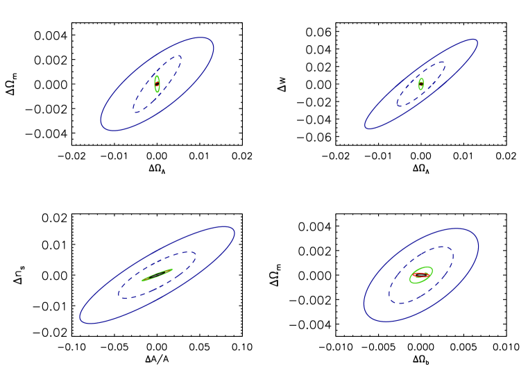
Figure 9: Predicted error ellipses ($\chi^{2}=2.2789$ or 68% probability) for six cosmological parameters. The fiducial model is $\Omega_{m}=0.3$, $\Omega_{\Lambda}=0.7$, $w=-1$, $n_{s}=1$, $\Omega_{b}=0.031$ and $\sigma_{8}=0.75$. The Hubble constant is fixed at $H_{o}=70\mbox{ km s${}^{-1}$}\mbox{ Mpc}^{-1}$. All constraints are obtained by marginalizing over the 4 parameters not shown in each plot. The solid blue ellipses are for a full-sky galaxy survey with $n_{g}=35\mbox{ arcmin}^{-2}$, $\sigma_{\epsilon}=0.3$ and a median redshift of $z=0.9$. The dashed blue ellipses are for a deeper survey with $n_{g}=100\mbox{ arcmin}^{-2}$, $\sigma_{\epsilon}=0.3$ and a median redshift of $z=1.23$. It would take the SNAP satellite roughly 30 years to complete a full-sky survey to the deeper depth. In all cases the galaxies are divided into three redshift bins as described in the text. The solid green ellipses are for shear maps from 21 cm alone at redshifts $z=10$ and 15. The dashed green ellipses are for the “optimal” 21 cm case with shear maps constructed for $z=10$, 30 and 100. For these calculations we assume pixel radius $\delta\theta=0.05$ arcmin and noise level $\sigma_{\tilde{\gamma}}(0)=0.02$, but the results are valid as long as $\sigma_{\tilde{\gamma}}(0)\delta\theta\lower 2.15277pt\hbox{$\;\buildrel<\over{\sim}\;$}0.017$ arcmin and $\delta\theta<0.5$ arcmin because in this case cosmic variance dominates the noise for all the $\ell$ values used. Modes $\ell=10$ to $\ell=10^{4}$ were used in deriving these constraints. The solid red ellipses are for the shallower galaxy survey combined with a 21 cm lensing survey at $z=10$ and 15. Finally, the solid black ellipse shows the “optimum” combination of the deeper galaxy lensing survey with 21 cm shear maps for $z=10$, 30 and 100. Figure 10 shows blow-ups of these plots so that the inner regions can be seen better. The line types are summarized in Table 1.

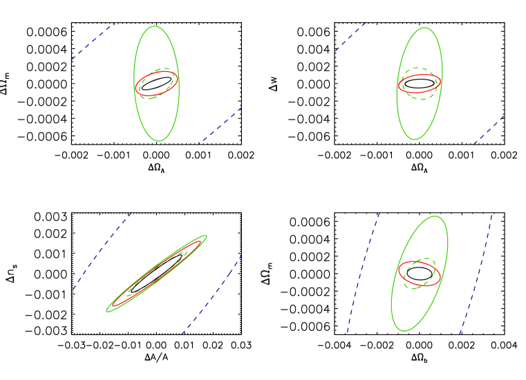
Figure 10: Blow-ups of the plots in figure 9.

To proceed we must choose a cosmological parameter space for exploration, a fiducial model to perturb around, and observational parameters for a set of representative surveys. For simplicity and for ease of comparison we follow the galaxy survey parameters chosen by Amara & Refregier (2006). In the current standard paradigm, the apparently accelerating expansion of the present universe is driven by dark energy, a near-uniform and dominant component of the cosmic energy density with effective equation of state $p=w\rho$ where $w<-1/3$ (Riess et al. 2004; Astier et al. 2006; Spergel et al. 2006). Dark energy modifies the lensing signal due to cosmic structure in two ways. It affects the angular size distance to a given redshift, which is given by the expression

$$r(z)=\frac{1}{H_{o}}\int_{0}^{z}\frac{dz^{\prime}}{E(z^{\prime})}~{},$$ (68)

where

$$E(z)=\left[\Omega_{m}(1+z)^{3}+\Omega_{\Lambda}\left(1+z\right)^{3(1+w)}+(1-\Omega_{m}-\Omega_{\Lambda})(1+z)^{2}\right]^{1/2}.$$ (69)

Here $\Omega_{\Lambda}$ denotes the dark energy density today in units of the critical density, and $w$ has been assumed to be constant. The second effect of dark energy results from its influence on the linear evolution of density fluctuations, which is given by

$$\frac{d^{2}\delta}{d\ln a^{2}}+\left(2+\frac{d\ln E(a)}{d\ln a}\right)\frac{d\delta}{d\ln a}-\frac{3}{2}\frac{\Omega_{m}}{a^{3}E(a)^{2}}\delta=0.$$ (70)

In addition to $\Omega_{m}$, $\Omega_{\Lambda}$ and $w$, we include in our cosmological parameter set the logarithmic slope or spectral index of the primordial power spectrum, $n_{s}$, the density of baryons, $\Omega_{b}$, and the normalization of the power spectrum on large scales $A$, which is proportional to $\sigma_{8}^{2}$. The baryon oscillations in the power spectrum are not calculated, so $\Omega_{b}$ only effects the overall shape. Note that we do not restrict ourselves to flat cosmologies, but we do fix the Hubble constant to $H_{o}=70$ km/s/Mpc, assuming this to be externally determined.

Table 1: Expected standard errors, $\sigma\times f_{\rm sky}^{1/2}$, in cosmological parameter estimates based on various lensing datasets.

	galaxies	galaxies	21 cm	21 cm	galaxies shallow	galaxies shallow	galaxies deep
	shallow	deep	z=10, 15	z=10, 30, 100	21 cm z=10	21 cm z=10, 15	21 cm z= 10, 30, 100
$\Delta\Omega_{m}$	0.0025	0.0015	0.0004	0.0001	0.0005	$9.0\times 10^{-5}$	$5.0\times 10^{-5}$
$\Delta\Omega_{\Lambda}$	0.009	0.004	0.00035	0.0002	0.001	0.0003	0.0002
$\Delta w$	0.03	0.02	0.004	0.001	0.002	0.0007	0.0003
$\Delta A$	0.06 $\times A$	0.03 $\times A$	0.01$\times A$	0.007 $\times A$	0.02 $\times A$	0.01 $\times A$	0.006 $\times A$
$\Delta n_{s}$	0.01	0.005	0.001	0.0007	0.003	0.001	0.0006
$\Delta\Omega_{b}$	0.004	0.002	0.0009	0.0005	0.002	0.0006	0.0004
line type in figures 9 & 10	solid blue	dashed blue	solid green	dashed green	-	solid red	solid black

Figures 9 and 10 show predicted error ellipses for various pairs of our set of six cosmological parameters and for various combinations of idealized 21 cm and galaxy lensing surveys. Whenever calculations are done for 21 cm lensing at a particular redshift the convergence is treated as if it where constant over the redshift range used in estimating it. For each plot we have marginalized over the remaining four parameters of our model set. In Table 1 we give corresponding $1\sigma$ uncertainties on individual parameters after marginalizing over the other five dimensions of our parameter space. The galaxy redshift distributions assumed here are the same as described at the end of section 4.2. When the galaxies are binned into several redshift intervals, we define these so as to obtain an equal number of galaxies in each bin. We also assume the full sky to be surveyed in all cases; for partial sky coverage the sizes of the uncertainties are approximately increased by a factor of $f_{\rm sky}^{-0.5}$. Apart from fixing the Hubble constant, no additional constraints from other observations are included.

In agreement with Amara & Refregier (2006) we find that a ambitious galaxy lensing survey could determine $\Omega_{\Lambda}$ and $n_{s}$ with an accuracy of about $\sim 0.01$, $\Omega_{b}$ with an accuracy of about 0.004, $\Omega_{m}$ with an accuracy of about 0.0025 and $w$, with an accuracy of about 0.03. An ideal survey going to a depth corresponding to 100 source galaxies per square arcminute over the whole sky (requiring about 30 years with the specifications of the SNAP satellite) would reduce these uncertainties by about a factor of two. Surveys covering only a fraction $f_{\rm sky}$ of the sky, would have uncertainties increased approximately in proportion to $f_{\rm sky}^{-1/2}$.

While these numbers are impressive, shear maps derived from 21 cm alone can provide considerably tighter constraints. All-sky maps derived from the signal around $z=10$ and $z=15$ will be limited by cosmic variance if their resolution and noise properties satisfy $\sigma_{\tilde{\gamma}}(0)\delta\theta<0.017$ arcmin, and will then determine $\Omega_{m}$ to an accuracy of $4\times 10^{-4}$, $\Omega_{\Lambda}$ to an accuracy of $3.5\times 10^{-4}$, and $w$ to an accuracy of 0.004. An ideal survey with source planes around $z=10$, 30 and 100 would reduce these even further, with $\Delta\Omega_{m}\sim 10^{-4}$, $\Delta\Omega_{\Lambda}\sim 0.0002$, $\Delta\Omega_{b}\sim 0.0005$, and $\Delta w\sim 0.001$.

Some parameter constraints are substantially improved by combining galaxy and 21 cm lensing, although most of the statistical weight comes from the latter. Thus combining the shallower galaxy survey considered above with the 21 cm survey at $z=10$ and 15, one finds that $\Omega_{\Lambda}$, $A$, $n_{s}$ and $\Omega_{b}$ are constrained about as well as by the 21 cm alone, while $w$ is constrained almost six times better and $\Omega_{m}$ four times better. Constraints on dark energy parameters are improved by including the galaxy lensing because dark energy primarily affects structure evolution at $z<1$. On the other hand, galaxy lensing alone gives comparatively poor constraints on these parameters unless a prior constraint on $\Omega_{m}$ is included. For parameters that affect only the matter power spectrum (e.g. $n_{s}$) 21 cm lensing has a larger comparative advantage. Of course it is not a question of one or the other. Clearly it is worth doing both galaxy and 21 cm lensing surveys to maximize the information gained and to spread the risk from unanticipated systematics.

It should be emphasized that this analysis does not exhaust the potential for constraining cosmological parameters using 21 cm or galaxy lensing. The dark energy model used here is overly simplified and may be unrealistic; some more physically based models imply appreciable effects at redshifts well beyond unity and so may be particularly well constrained by 21 cm surveys (Caldwell et al. 2003; Doran, Schwindt & Wetterich 2001). Other datasets, notably CMB observations and supernova surveys, constrain cosmological parameters in different ways than gravitational lensing, and will be much improved by the time surveys of the type discussed in this section are completed. Combining results from all these sources will give stringent tests for the presence of systematics and will provide tighter and more robust final constraints if overall consistency is found. Our knowledge of many cosmological parameters is limited by degeneracies which are drastically reduced when different types of observation are combined in this way.

6 observations

So far we have considered idealized observations where the irreducible noise dominates and the bandwidth is smaller than the intrinsic correlation length of the brightness temperature. This will be the best any experiment can do and, as we showed, will be reached when the noise in the temperature map is small compared to the temperature fluctuations in each frequency channel. This irreducible noise depends only on the shape of the temperature correlation function. Realistic observations, at least in the near future, will have foreground noise levels that are comparable to or larger than the intrinsic fluctuations in the brightness temperature. In this case the noise in the lensing map will depend more sensitively on the parameters of the telescope and on the level and statistical properties of the brightness temperature fluctuations. We now discuss these factors in more detail.

The observations will be carried out with radio interferometers and thus in visibility space. As a result, when calculating the performance of telescopes it is easier to work in Fourier-space. For this section we adopt the formalism of appendix C for convenience. Equations (104) and (107) give the noise in the $\kappa$ estimate as a function of the power spectrum of foreground noise, $C_{\ell}^{N}(\nu)$, and the power spectrum of the brightness temperature, $\overline{C}_{\ell}(\nu)$.

The noise in each visibility will have a thermal component and a component from imperfect foreground subtraction. We will model only the thermal component. If the telescopes in the array are uniformly distributed on the ground the average integration time for each baseline will be the same and the power spectrum of the noise will be

$$C_{\ell}^{N}=\frac{2\pi}{\Delta\nu t_{o}}\left(\frac{T_{\rm sys}\lambda}{f_{\rm cover}D_{\rm tel}}\right)^{2}=\frac{(2\pi)^{3}T_{\rm sys}^{2}}{\Delta\nu t_{o}f_{\rm cover}^{2}\ell_{\rm max}(\nu)^{2}}$$ (71)

(Zaldarriaga et al. 2004; Morales 2005; McQuinn et al. 2006) where $T_{\rm sys}$ is the system temperature, $\Delta\nu$ is the bandwidth, $t_{o}$ is the total observation time, $D_{\rm tel}$ is the diameter of the array and $\ell_{\rm max}(\lambda)=2\pi D_{\rm tel}/\lambda$ is the highest multipole that can be measure by the array as set by the largest baselines. $f_{\rm cover}$ is the total collecting area of the telescopes divided by $\pi(D_{\rm tel}/2)^{2}$, the covering fraction. Other telescope configurations are possible which would make the noise unequally distributed in $\ell$, but we will consider only this uniform configuration here. For our calculations we will use $T_{\rm sys}=200$ K.

There are several relevant telescopes proposed or under construction. The 21 Centimeter Array (21CMA, formerly known as PAST) has $f_{\rm cover}\sim 0.1$ and $\ell_{\rm max}\sim 10^{3}$ giving it a resolution of about 10 arcmin. The Mileura Widefield Array (MWA) Low Frequency Demonstrator (LFD) will operate in the 80-300 MHz range with $D_{\rm tel}\simeq 1.5$ km and $f_{\rm cover}\sim 0.1$. For LOFAR (Low Frequency Array) the core array will have $f_{\rm cover}\sim 0.016$ and $D_{\rm tel}\sim 2$ km. LOFAR’s extended baselines, out to 350 km and possibly larger, are not expected to be useful for high redshift 21 cm observations because of the small $f_{\rm cover}$ of the extended array, although they will be used in foreground subtraction. It is anticipated that it will be able to detect 21 cm emission out to a redshift of $z\simeq 11.5$, but sensitivity limitations will make mapping very difficult. Plans for SKA (Square Kilometer Array) have not been finalized, but it is expected to have $f_{\rm cover}\sim 0.02$ out to a diameter of $\sim 6$ km ($\ell_{\rm max}\sim 10^{4}$) and sparse coverage extending out to 1,000-3,000 km. The lowest frequency currently anticipated is $\sim 100$ MHz which corresponds to $z\sim 13$. It is anticipated that the core will be able to map the 21 cm emission with a resolution of $\delta\theta=\Delta\theta/2\sim 0.5\mbox{ arcmin}$. For reference what we call the pixel-width is given by $\Delta\theta=2\delta\theta\sim\pi/\ell_{\rm max}$ or $1.08\times 10^{4}/\ell_{\rm max}$ arcmin. One arcminute (fwhm) corresponds to baselines of 7.9 km and 73 km at redshifts of 10 and 100 respectively. For our calculation we will concentrate only on an SKA-like array with $D_{\rm tel}=6$ km and a redshift range out to $z=13$ since the smaller planned telescopes will not be capable of mapping mass at high fidelity.

The fluctuations in the brightness temperature depends on the spin temperature, the ionization and the density of HI through

$$\delta T_{b}\simeq 24(1+\delta_{b})x_{\rm H}\left(\frac{T_{s}-T_{\rm CMB}}{T_{s}}\right)\left(\frac{\Omega_{b}h^{2}}{0.02}\right)\left(\frac{0.15}{\Omega_{m}h^{2}}\frac{1+z}{10}\right)^{1/2}\mbox{ mK}$$ (72)

(Field 1959; Madau, Meiksin & Rees 1997). As is commonly done, we will assume that the spin temperature is much greater than the CMB temperature. This leaves fluctuations in the ionization fraction, $x_{H}$, and the baryon density $\delta_{b}=(\rho_{b}-\overline{\rho}_{b})/\overline{\rho}_{b}$ as the sources of fluctuations. We will make the simplifying assumption that $x_{\rm H}=1$ until the universe is very rapidly and uniformly reionized. Realistically, the reionization process will be inhomogeneous and may extend over a significant redshift range. This will increase $\overline{C}_{\ell}(\nu)$ by perhaps a factor of 10 on scales larger the characteristic size of the ionized bubbles and thus might be expected to reduce the noise in $\tilde{\kappa}$ significantly. However, we have derived the noise in the lensing map by approximating the fourth order statistics of $\delta T_{b}$ as they would be for a Gaussian random field. If this is still a good approximation the lensing noise will be reduced. This is uncertain, however, since during reionization the field will clearly not be Gaussian, especially when the neutral fraction is low. A definitive resolution of these uncertainties will not be available until the observations are done. Here we model fluctuations in the baryons in the same way as in section 3.2 with linear structure formation and redshift distortions.

Figure 11: The signal-to-noise, $\sigma_{\tilde{\kappa}}(\delta\Theta,\Delta\nu)/\sigma_{\kappa}(\delta\Theta)$, ratio for an SKA-like observation as a function of bandwidth and patch size. In all cases the contours are 1, 2, 4 and 8$\sigma$ (when visible). The solid contours are for a covering fraction of $f_{\rm cover}=0.025$ and the dashed contours are for $f_{\rm cover}=0.018$. The dotted contours are the signal-to-noise ratio for brightness temperature with the same telescope parameters and $f_{\rm cover}=0.018$. The other telescope parameters are $T_{\rm sys}=200$ K, $D_{\rm tel}=6$ km, $t_{o}=90$ days and the universe is assumed to be neutral in the redshift range $z=7$ to 13 in all cases.

Figure 11 shows the signal-to-noise ratio, defined as $\sigma_{\tilde{\kappa}}(\delta\Theta,\Delta\nu)/\sigma_{\kappa}(\delta\Theta)$, for our SKA-like telescope. For the assumptions taken here the telescope should be able to make images ($2\sigma$) of the dark matter on $1.3$ to 2.5 arcmin scales in 90 days ($f_{\rm cover}=0.018$ to 0.025). These values are not too far from the optimal values and increasing the telescope’s covering fraction or resolution would markedly improve upon these.

Unlike in the irreducible noise only case shown in figure 6, when thermal noise is added the noise in $\tilde{\kappa}$ does not go to an asymptotic value at small $\delta\Theta$. This is because the noise increases very rapidly near the maximum resolution of the telescope because of a combination of effects. First the intrinsic temperature power spectrum goes down at $\ell\lower 2.15277pt\hbox{$\;\buildrel>\over{\sim}\;$}1000$. $\overline{C}_{\ell}(\nu)$ is also suppressed by a factor of $\sim 1/\Delta\nu$ when $\ell>D(z)/\delta r$ where $\delta r$ is physical width corresponding to the bandwidth. In addition, for a fixed baseline the highest resolution is attained for only a limited range of frequency which limits the number of redshift bins. With the parameters adopted, the cross-correlation in the temperature between frequency channels never becomes important because the noise generally dominates when $\Delta\nu$ is small and it is assumed to have no cross-correlation between channels.

As can be seen from figure 11, there is an optimal bandwidth for measuring lensing. This comes about because at large bandwidths the number of independent frequency bins is limited. At small bandwidth the the signal-to-noise goes down because $C_{\ell}^{N}$ goes up faster than $\overline{C}_{\ell}$ with decreasing $\Delta\nu$ for scales $\ell<D(z)/\delta r$. This optimal bandwidth is $\sim 0.05$ MHz for our examples. If there is more structure on smaller scales, such as when there are ionized bubbles, the optimal frequency will decrease.

The optimal bandwidth for lensing is generally smaller than the optimal bandwidth for measuring the brightness temperature itself as can also be seen in figure 11. At the optimal bandwidth the lensing map can have good fidelity while the temperature map is noise dominated on the same scale. This is a somewhat counter-intuitive situation which reflects the fact that it is better to get more independent redshift slices at low signal-to-noise than to image the temperature in fewer channels. With a wider bandwidth the temperature can be imaged on the same angular scale as the mass distribution. This indicates that it may be advantageous to use several bandwidths simultaneously.

There are many additional challenges to observing 21 cm radiation from high redshift. The galactic foreground from synchrotron emission is about four orders of magnitude brighter than the 21 cm signal at $\sim 180$ MHz and goes up with decreasing frequency as $\nu^{-2.6}$. Both this emission and extragalactic foreground sources can, however, be cleaned from the data because they are much smoother in frequency space (and also in position on the sky for the Galactic foreground) than the 21 cm signal itself. At large frequency separations foreground emission may also decorrelate. Generally, foregrounds pose no more of a problem for mass-mapping than for direct mapping of the 21 cm itself. Rapid increases in foreground emission and in the refractive index of the ionosphere with decreasing frequency make observations at higher redshift progressively more difficult. The high-redshift 21 cm absorption ($z\lower 2.15277pt\hbox{$\;\buildrel>\over{\sim}\;$}30$) will be very difficult to observe and there are no mature plans to do so at this time. The ionosphere is opaque below $\sim 10$ MHz or $z\lower 2.15277pt\hbox{$\;\buildrel>\over{\sim}\;$}150$, so in principle all lower redshifts are accessible from the ground. In practice, the high, time-dependent index of refraction will make it difficult to go beyond $\sim 60$ MHz without major advances in telescope technology. The ultimate high redshift 21 cm telescope would be located on the far side of the Moon where the absence of terrestrial interference or an ionosphere would allow access to higher redshifts. However, the large collecting area required would make this both technically challenging and expensive.

Much will depend on future instrument design and the as yet unknown characteristics of the 21 cm absorption/emission, particularly around the epoch of reionization. Despite this, the planned specifications for SKA may enable it to make high-fidelity maps of the matter distribution and if enough area can be surveyed very good statistical information should be accessible. Realistic upgrades to the collecting area and array size would greatly improve its ability to make mass maps.

7 conclusion

We have shown that when low-frequency radio telescopes become sufficiently powerful to map the signal from high-redshift 21 cm emission/absorption within a bandwidth of $\sim 0.05$ MHz, the data will necessarily be good enough to map the gravitational shear due to foreground matter. Increasing the resolution of the telescope reduces the intrinsic noise in the shear map both because of the number of statistically independent redshift slices increases and because the number of independent patches on the sky increases. As a result, 21 cm lensing offers the potential of producing high resolution, high signal-to-noise images of the cosmic mass distribution. Such images would be of enormous value for the study of cosmology and galaxy formation.

For the specific problem of estimating cosmological parameters the requirements on resolution and redshift range are not particularly demanding, but survey area is of great importance. Even for a full-sky survey with a pixel of radius $\delta\theta=1$ arcmin (2 arcmin fwhm) and 10% noise per pixel, the shear power spectrum would be cosmic variance dominated up to $\ell\sim 10^{3}$. The cosmic variance limit is probably achievable up to $\ell\sim 10^{4}$ with an array of $\sim 5$ km in diameter and a covering factor of several percent. Cross-correlating several redshift slices with each other and with galaxy lensing surveys over a significant portion of the sky would begin a new era of very high precision cosmology.

The study of structure formation would benefit particularly from higher resolution observations, however. If a resolution of $\sim 6$ arcsec (fwhm) could be achieved, every halo more massive than the Milky Way’s would be clearly visible back to $z\sim 10$. Even with a resolution of $\sim 1$ arcmin (fwhm) all the halos $\lower 2.15277pt\hbox{$\;\buildrel>\over{\sim}\;$}2\times 10^{13}\mbox{ M}_{\odot}$ should be individually detected. Connecting these mass maps to images of emission at other wavelengths would provide a tremendous wealth of information about the evolution of structure and the formation of galaxies.

RBM would like to thank B. Ciardi, P. Madau and H. Sandvik for very useful discussions. We would also like to thank U. Seljak and O. Zahn for very useful comments.

Appendix A parameter estimation and visibility space

The observations of 21 cm emission/absorption will be done with radio interferometers so it is appropriate to make an explicit connection between the observables from such an instrument and the quantities used in this paper. The flat sky approximation greatly simplifies the mathematics and is well justified for the angular scales of interest here. A radio interferometer measures the visibility, $V({\bf u})$, which in our case is related to the spin temperature by

$$V({\bf u}) = \int d\boldsymbol{\theta}~{}A(\boldsymbol{\theta})T((\boldsymbol{\theta})e^{i2\pi{\bf u}\cdot\boldsymbol{\theta}}$$ (73)

$$= \int d^{2}{w}\tilde{A}({\bf w})\tilde{T}({\bf u}-{\bf w})$$ (74)

where $A(\theta)$ is the primary beam of the telescopes which is typically normalized to one at its peak ($\boldsymbol{\theta}=0$) which gives its Fourier transform, $\tilde{A}({\bf u})$, a normalization of one in ${\bf u}$-space. Units of temperature are used here (flux density units have a factor of $2k_{\rm B}/\lambda^{2}$). Tildes signify Fourier transforms. The size of the primary beam dictates the area covered on the sky in one “pointing” of the telescopes. The separation of the antennas and the position on the sky dictate ${\bf u}$.

The correlation in the visibilities is given by

$$C^{V}_{ij} \equiv \langle V^{*}({\bf u}_{i})V({\bf u}_{j})\rangle$$ (75)

$$= \int d^{2}{w}~{}\tilde{A}^{*}({\bf u}_{i}-{\bf w})\tilde{A}({\bf u}_{j}-{\bf w})S({\bf w})+\delta_{ij}C^{N}_{\bf u}$$ (76)

$$\simeq S({\bf u}_{i})W_{ij}+\delta_{ij}C^{N}_{\bf u}$$ (77)

where $S({\bf u})$ is the intrinsic (cross-)power spectrum of the temperature and $C^{N}_{\bf u}$ is the noise. It has been assumed that the temperature field is isotropic. Equation (77) defines the window, $W_{ij}(w)$, that makes the visibilities correlated. This in effect defines the resolution in ${\bf u}$-space. Correlations will only exist when $\Delta{\bf u}\equiv|{\bf u}_{i}-{\bf u}_{j}|$ is less than twice the width of $\tilde{A}({\bf u})$, i.e. the smaller the telescopes are the narrower $\tilde{A}({\bf u})$ will be and the higher the resolution. This width will be denoted $\sigma_{u}({\bf u})$. It has been assumed in equation (77) that the intrinsic power spectrum does not change very much on the scale of $\sigma_{u}$. The coordinate ${\bf u}$ is conjugate to the angle on the sky $\boldsymbol{\theta}$ so the resolution is linked to the area covered on the sky by $f_{\rm sky}\simeq(2\pi\sigma_{u})^{-2}$.

The visibility power spectrum can be related to the spherical harmonic power spectrum through

$$u^{2}S(u) = \frac{u}{2\pi}\sum_{\ell}(2\ell+1)C_{\ell}J_{2\ell+1}(4\pi u)$$ (78)

$$\simeq \left.\frac{\ell(1+\ell)}{(2\pi)^{2}}C_{\ell}\right|_{\ell=2\pi u}$$ (79)

where the second approximation is very good for $\ell\lower 2.15277pt\hbox{$\;\buildrel>\over{\sim}\;$}60$ (White et al. 1999). If there were just one visibility measured the Fisher matrix would be

$${\bf F}({\bf u})_{ab}=\frac{1}{2}{\rm tr}\left[(C^{V}_{\bf u})^{-1}C^{V}_{\bf u},_{a}(C^{V}_{\bf u})^{-1}C^{V}_{\bf u},_{b}\right]$$ (80)

(see Tegmark, Taylor & Heavens 1997, for a review of likelihood methods in astronomy). Visibilities within $\sim\sigma_{u}$ of each other will be correlated, but an estimate of the total Fisher matrix can be made by assuming one measurement per correlated region which gives

$${\bf F}_{ab} = \sum_{\bf u}{\bf F}({\bf u})_{ab}\simeq\int\frac{d^{2}{u}}{\sigma_{u}^{2}}{\bf F}({\bf u})_{ab}$$ (81)

$$\simeq \frac{1}{(2\pi\sigma_{u})^{2}}\sum_{\ell m}{\bf F}(\ell=2\pi|{\bf u}|)_{ab}$$ (82)

$$\simeq f_{\rm sky}\sum_{\ell}(2\ell+1){\bf F}(\ell=2\pi u)_{ab}.$$ (83)

This is the formula (66) in section 5 used to calculate cosmological parameter constraints. It can be seen that the $f_{\rm sky}$ factor comes from the correlations or resolution in visibility space. A more sophisticated treatment would allow for partially correlated visibilities within $\sigma_{u}$ of each other which would reduce the noise further. The Fisher matrix is an estimate of the expected inverse correlation matrix in the model parameters at the maximum likelihood solution. Thus $\left({\bf F}^{-1}\right)_{aa}$ is an estimate of the error in the parameter $a$ after marginalizing over the other parameters. This formalism as outlined here in terms of the temperature, but it is equally valid for the lensing shear or convergence.

The size of individual antennas in future radio telescope arrays are expected to be of order a few wavelengths or smaller as in the case of dipole antennas. In this case the primary beam covers almost the whole hemisphere. However, subtracting interference and handling the huge data rate will probably require synthesizing a much smaller beam. In addition, the subtraction of galactic foregrounds will probably not be possible in some regions near the galactic plane. For these reasons the sky fraction, $f_{\rm sky}$, and the shape of the observed fields will be limited for a single pointing of the telescope beam. The sky fraction and thus the $\ell$-space resolution can be increased with multiple pointing or mosaicking.

Appendix B lensing in Fourier space

The temperature on the sky is to first order

$$T(\boldsymbol{\theta},\nu)={\mathcal{T}}(\boldsymbol{\theta},\nu)+\vec{\nabla}\Phi(\boldsymbol{\theta})\cdot\vec{\nabla}{\mathcal{T}}(\boldsymbol{\theta},\nu)$$ (84)

where ${\mathcal{T}}(\boldsymbol{\theta},\nu)$ is the temperature before lensing and $\Phi({\bf L})$ is the lensing potential defined so that the deflection angle is $\boldsymbol{\alpha}(\boldsymbol{\theta})=\vec{\nabla}\Phi(\boldsymbol{\theta})$. The Fourier transform of this is

$$T(\boldsymbol{\ell},\nu)={\mathcal{T}}(\boldsymbol{\ell},\nu)-\int\frac{d^{2}{\ell^{\prime}}}{(2\pi)^{2}}~{}\boldsymbol{\ell}^{\prime}\cdot(\boldsymbol{\ell}-\boldsymbol{\ell}^{\prime})\Phi(\boldsymbol{\ell}^{\prime}){\mathcal{T}}(\boldsymbol{\ell}-\boldsymbol{\ell}^{\prime},\nu)$$ (85)

and, as a result, to first order

$$\left\langle T(\boldsymbol{\ell},\nu)T^{*}(\boldsymbol{\ell}-{\bf L},\nu^{\prime})\right\rangle=\left[{\bf L}\cdot\boldsymbol{\ell}\,C_{\ell}(\nu,\nu^{\prime})+{\bf L}\cdot({\bf L}-\boldsymbol{\ell})\,C_{|\ell-L|}(\nu,\nu^{\prime})\right]\Phi({\bf L})$$ (86)

where ${\bf L}\neq 0$ and the average is over realizations of the temperature field while keeping the lensing potential fixed (Hu & Okamoto 2002). Note that if the noise is homogeneous it will drop out of this equation and the $C_{\ell}$’s will be only the power spectrum of the fluctuations in brightness temperature.

The observed temperature is always binned into frequency channels or bands and smoothed by the telescope’s beam. This observed temperature is

$$\overline{T}(\boldsymbol{\ell},\nu) = \int dr^{\prime}q_{\nu}(r^{\prime},\Delta\nu)\int d^{2}l^{\prime}\tilde{A}(\boldsymbol{\ell}^{\prime}-\boldsymbol{\ell})T(\boldsymbol{\ell}^{\prime},\nu^{\prime})$$ (87)

$$= \frac{1}{D(\nu)^{2}}\int d^{2}l^{\prime}\tilde{A}(\boldsymbol{\ell}^{\prime}-\boldsymbol{\ell})\int\frac{dk}{2\pi}T_{21}\left(\frac{\boldsymbol{\ell}^{\prime}}{D(\nu)},k\right)\tilde{q}_{\nu}(k,\nu)$$ (88)

where the $q_{\nu}(r^{\prime},\Delta\nu)$ is the response function for the band centered on $\nu$, $T_{21}$ is the 3D Fourier transform of the brightness temperature and

$$\tilde{q}_{\nu}(k,\nu) = \int dr^{\prime}q_{\nu}(r^{\prime},\Delta\nu)e^{ikr^{\prime}}$$ (89)

$$\simeq j_{o}\left(\frac{k\delta r(\nu,\Delta\nu)}{2}\right)e^{ikr(\nu)}$$ (90)

with

$$\delta r(\nu,\Delta\nu)=\frac{2}{H_{o}\sqrt{\Omega_{m}\nu_{o}}}\left(\sqrt{\nu+\Delta\nu/2}-\sqrt{\nu-\Delta\nu/2}\right).$$ (91)

In (90) the response function is taken to be a boxcar shape with sharp edges at $\nu+\Delta\nu/2$ and $\nu-\Delta\nu/2$. In (91) the fact that the universe is matter dominated at the time of the 21 cm emission/absorption is used to express the radial distances in terms of frequency.

As a result of beam smearing relation (86) will become

$$\left\langle\overline{T}(\boldsymbol{\ell},\nu)\overline{T}^{*}(\boldsymbol{\ell}-{\bf L},\nu^{\prime})\right\rangle=(2\pi)^{2}\int d^{2}{\ell}^{\prime}\tilde{A}(\boldsymbol{\ell}^{\prime})\tilde{A}^{*}(\boldsymbol{\ell}^{\prime}+{\bf L})\overline{C}_{\ell+\ell^{\prime}}~{}~{}~{}~{}~{}~{}~{}~{}~{}~{}~{}~{}~{}~{}~{}~{}~{}~{}~{}~{}~{}~{}~{}~{}~{}~{}~{}~{}~{}~{}~{}~{}~{}~{}~{}~{}~{}~{}~{}~{}~{}~{}~{}~{}~{}~{}~{}~{}~{}~{}~{}~{}~{}~{}~{}~{}~{}~{}~{}~{}~{}~{}~{}~{}~{}~{}~{}~{}~{}$$ (92)

$$+\int d^{2}{\ell}^{\prime\prime}\Phi(\boldsymbol{\ell}^{\prime\prime})\int d^{2}{\ell}^{\prime}\tilde{A}(\boldsymbol{\ell}^{\prime})\tilde{A}^{*}(\boldsymbol{\ell}^{\prime}-\boldsymbol{\ell}^{\prime\prime}+{\bf L})\left\{\left(\boldsymbol{\ell}^{\prime\prime}\cdot(\boldsymbol{\ell}+\boldsymbol{\ell}^{\prime})\overline{C}_{\ell+\ell^{\prime}}(\nu,\nu^{\prime})-\boldsymbol{\ell}^{\prime\prime}\cdot(\boldsymbol{\ell}+\boldsymbol{\ell}^{\prime}-\boldsymbol{\ell}^{\prime\prime})\overline{C}_{\ell+\ell^{\prime}-\ell^{\prime\prime}}(\nu,\nu^{\prime})\right)\right\}$$ (93)

where the correlations between temperature modes before lensing and beam smearing

$$\overline{C}_{\ell}(\nu,\nu^{\prime}) = \frac{1}{D(\nu)^{2}}\int dk~{}P_{21}\left(\sqrt{\frac{\ell^{2}}{D(\nu)^{2}}+k^{2}},z(\nu)\right)\tilde{q}_{\nu}(k,\nu)\tilde{q}^{*}_{\nu}(k,\nu^{\prime})$$ (94)

It is assumed that $D(\nu)$ does not change significantly between frequencies that are significantly correlated. A more rigorous derivation of (94) is in spherical harmonic space as has been done by Zaldarriaga et al. (2004), but for the scales of important here the difference is very small and (94) is considerably easier to evaluate.

There are two effects that make (92) and (93) different from the Hu & Okamoto (2002) result (86). The first term (92) represents an aliasing effect caused by the finite size of the beam. This will cause a false signal on scales approaching the size of the beam or surveyed region, $L\lower 2.15277pt\hbox{$\;\buildrel<\over{\sim}\;$}2\pi\sigma_{u}$, that will need to be subtracted. The second term (93) is a kind of smoothing of the lensing potential over a scale of $\sim 2\pi\sigma_{u}$. In the limit of a very narrow beam, a large area in angle, the relation (86) is recovered except with the frequency binned power spectra. Thus the observations will really measure a lensing potential that is smoothed in Fourier-space in a rather complicated fashion.

Appendix C convergence estimators

In the main text of this paper we used a real-space estimators for the shear and convergence, $\hat{\gamma}_{i}(\boldsymbol{\theta})$. We consider this the most intuitive and instructive approach. In the weak lensing limit the shear map can be converted to a convergence map because they are both related to a single lensing potential by differential operators. This is commonly done for galaxy lensing surveys (see Bartelmann & Schneider (2001) for a review). The most straightforward method is to Fourier transform the shear map, multiply by $\ell$ dependent factors and then transform back to a convergence map (Kaiser & Squires 1993). Averaging this with the $\hat{\gamma}_{3}$ map would produce a convergence map with less noise than the $\hat{\gamma}_{3}$ map alone. However, the gain in noise will not be as great as in the galaxy lensing case because in the 21 cm lensing case the Fourier modes of $\hat{\gamma}_{1}$ and $\hat{\gamma}_{2}$ are correlated unlike in the galaxy case. Probably a more practical approach from a technical point of view is to go directly from visibility space to a convergence map in real-space.

Many convergence estimators in visibility or Fourier space are possible. Our real-space estimators can be Fourier transformed to make a set of estimators for the Fourier modes of shear and convergence, but the Fourier estimator of Hu & Okamoto (2002) has the advantage of having the lowest noise level for one frequency bin if the temperature distribution is Gaussian and the beam is infinitely large (in angle). Zahn & Zaldarriaga (2006) find an estimator in both angular Fourier-space and frequency Fourier-space which is optimal with the added assumption that the frequency Fourier modes are statistically independent and Gaussian distributed. The statistical independence of the modes will break down because of binning in frequency and to a lesser extent because of the finite range in frequency. For this reason it is difficult to determine how bandwidth will affect the noise in their estimator. Instead we choose to use the Hu & Okamoto (2002) estimator for each frequency band and then weight each band.

We consider a second-order estimator for the shear or convergence of the form

$$\tilde{\gamma}_{i}({\bf L}) = \sum_{\nu}\int d^{2}\boldsymbol{\ell}~{}\Gamma_{i}(\boldsymbol{\ell},{\bf L},\nu)~{}\overline{T}(\boldsymbol{\ell},\nu)\overline{T}^{*}(\boldsymbol{\ell}-{\bf L},\nu).$$ (95)

where, as in the main text, $\tilde{\gamma}_{1,2}$ are estimators for the two components of shear and $\tilde{\gamma}_{3}$ is an estimator for the convergence. In this case the estimators are of the form

$$\Gamma_{i}(\boldsymbol{\ell},{\bf L},\nu)=D_{i}({\bf L})\omega(\nu,{\bf L})\chi(\boldsymbol{\ell},{\bf L},\nu)$$ (96)

where

$$D_{i}({\bf L})=\left\{\begin{array}[]{c}\left(L_{1}^{2}-L_{2}^{2}\right)\\ 2L_{1}L_{2}\\ |{\bf L}|^{2}\end{array}\right.$$ (100)

The function $\chi(\boldsymbol{\ell},{\bf L},\nu)$ is proportional to the Hu & Okamoto (2002) estimator

$$\chi(\boldsymbol{\ell},{\bf L},\nu)=\frac{\left[{\bf L}\cdot\boldsymbol{\ell}\,\overline{C}_{\ell}(\nu)+{\bf L}\cdot({\bf L}-\boldsymbol{\ell})\,\overline{C}_{|\ell-L|}(\nu)\right]}{\overline{C}^{T}_{\ell}(\nu)\overline{C}^{T}_{|\ell-L|}(\nu)}$$ (101)

where $\overline{C}^{T}_{\ell}(\nu)$ is the power spectrum of the actual temperature while $\overline{C}_{\ell}(\nu)=\overline{C}^{T}_{\ell}(\nu)+\overline{C}^{N}_{\ell}(\nu)$ is the observed power spectrum which includes noise and $\omega(\nu,{\bf L})$ is a weight that is to be determined.

In the limit of an infinitely large beam the correlation between modes is

$$\left\langle\hat{\gamma}_{i}\left({\bf L}\right)\hat{\gamma}_{j}^{*}\left({\bf L}^{\prime}\right)\right\rangle = 2(2\pi)^{4}\delta\left({\bf L}-{\bf L}^{\prime}\right)D_{i}({\bf L})D_{j}({\bf L})\sum_{\nu}\sum_{\nu^{\prime}}\omega(\nu)\omega(\nu^{\prime})\int d^{2}{\ell}~{}\chi\left(\boldsymbol{\ell},{\bf L}\right)\chi\left(\boldsymbol{\ell},{\bf L}\right)\overline{C}^{T}_{\ell}(\nu,\nu^{\prime})\overline{C}^{T}_{|\ell-L|}(\nu,\nu^{\prime})$$ (102)

$$= (2\pi)^{2}\delta\left({\bf L}-{\bf L}^{\prime}\right)D_{i}({\bf L})D_{j}({\bf L})N^{ij}_{\hat{\gamma}}(L)$$ (103)

It has been assumed here that the temperature is Gaussian distributed so that the fourth moment can be written as products of second moments. The finite beam will cause correlations in the noise $\langle\gamma_{i}({\bf L})\gamma_{i}({\bf L}+\delta{\bf L})\rangle\neq 0$ when $\delta L\lower 2.15277pt\hbox{$\;\buildrel<\over{\sim}\;$}2\pi\sigma_{u}$. The expression for these correlations is lengthy, but easily worked out. In general there will be a correlation between the modes for different components of shear, unlike in real-space. An image can be constructed by Fourier transforming (95) to real-space with a smoothing window. The noise at a point on this image will be

$$\sigma^{2}_{i}(\delta\Theta)=\int\frac{d^{2}L}{(2\pi)^{2}}\left|\tilde{W}({\bf L},\delta\Theta)\right|^{2}D_{i}({\bf L})^{2}N_{\hat{\gamma}}(L)$$ (104)

where $\tilde{W}({\bf L},\delta\Theta)$ is the Fourier transform of the smoothing function. This implies that $\sigma^{2}_{\kappa}(\delta\Theta)=2\sigma^{2}_{1}(\delta\Theta)=2\sigma^{2}_{2}(\delta\Theta)$ in contrast to the noise in the real-space estimators.

As in the real-space version, the optimal frequency weights, $\omega(\nu)$, are complicated in general, but they simplify if we make the approximation that each frequency bin is statistically independent. If we minimize the diagonal entries of (102) while requiring that the average of (95) with (86) reproduce the shears and the convergence, we find

$$\omega(\nu)=\frac{1}{2}\left[\sum_{\nu}\int d^{2}{\ell}\frac{\left[{\bf L}\cdot\boldsymbol{\ell}\,\overline{C}_{\ell}(\nu)+{\bf L}\cdot({\bf L}-\boldsymbol{\ell})\,\overline{C}_{|\ell-L|}(\nu)\right]^{2}}{\overline{C}^{T}_{\ell}(\nu)\overline{C}^{T}_{|\ell-L|}(\nu)}\right]^{-1}$$ (105)

These weights can be reinserted in expression (102), but now allowing for correlations between frequencies,

$$N_{\hat{\gamma}}(L)=\frac{(2\pi)^{2}}{2}\left[\sum_{\nu}\int d^{2}\ell~{}\chi(\boldsymbol{\ell},{\bf L},\nu)^{2}\overline{C}^{T}_{\ell}(\nu)\overline{C}^{T}_{|\ell-L|}(\nu)\right]^{-2}\sum_{\nu}\sum_{\nu^{\prime}}\int d^{2}{\ell}~{}\chi(\boldsymbol{\ell},{\bf L},\nu)\chi(\boldsymbol{\ell},{\bf L},\nu^{\prime})\overline{C}^{T}_{\ell}(\nu,\nu^{\prime})\overline{C}^{T}_{|\ell-L|}(\nu,\nu^{\prime})$$ (106)

This can be rewritten in the suggestive form

$$N_{\hat{\gamma}}(L)=\frac{(2\pi)^{2}N_{\nu}}{2N^{\rm eff}_{\nu}(L)}\left[\sum_{\nu}\int d^{2}\ell~{}\frac{\left[{\bf L}\cdot\boldsymbol{\ell}\,\overline{C}_{\ell}(\nu)+{\bf L}\cdot({\bf L}-\boldsymbol{\ell})\,\overline{C}_{|\ell-L|}(\nu)\right]^{2}}{\overline{C}^{T}_{\ell}(\nu)\overline{C}^{T}_{|\ell-L|}(\nu)}\right]^{-1}$$ (107)

where

$$N^{\rm eff}_{\nu}(L) = N_{\nu}\frac{\sum_{\nu}\int d^{2}\ell~{}\chi(\boldsymbol{\ell},{\bf L},\nu)^{2}\overline{C}^{T}_{\ell}(\nu)\overline{C}^{T}_{|\ell-L|}(\nu)}{\sum_{\nu}\sum_{\nu^{\prime}}\int d^{2}{\ell}~{}\chi(\boldsymbol{\ell},{\bf L},\nu)\chi(\boldsymbol{\ell},{\bf L},\nu^{\prime})\overline{C}^{T}_{\ell}(\nu,\nu^{\prime})\overline{C}^{T}_{|\ell-L|}(\nu,\nu^{\prime})}$$ (108)

$$= \frac{(\nu_{2}-\nu_{1})}{\Delta\nu_{L}}$$ (109)

which is essentially the Zahn & Zaldarriaga (2006) estimator except for the $N_{\nu}/N^{\rm eff}_{\nu}(L)$ factor. $N^{\rm eff}_{\nu}(L)$ is the effective number of independent frequency bins. Line (109) is an alternative definition of the frequency correlation length. If the frequency bins are uncorrelated $N^{\rm eff}_{\nu}(L)=N_{\nu}$ and $\Delta\nu_{L}=\Delta\nu$, but if there are correlations between bins $N^{\rm eff}_{\nu}(L)<N_{\nu}$ and $\Delta\nu_{L}>\Delta\nu$. The irreducible noise limit discussed in section 3 corresponds to the case where $\overline{C}_{\ell}(\nu)=\overline{C}^{T}_{\ell}(\nu)$ and to infinitely narrow frequency bins.

In actual data the temperature distribution will not be Gaussian, the foregrounds will not be perfectly subtracted which will produce spurious correlations in frequency, there will be holes in the surveyed area caused by point source subtraction, there will be a finite and irregular beam, and the coverage of $u$-$v$ plane will not be complete. All these complications making it unclear at this time what estimator will be the best choice for real data.

References

- [Amara & Refregier 2006] Amara, A. & Refregier, A. 2006, preprint astro-ph/0610127, submitted to MNRAS
- [Astier, Guy, Regnault, Pain, Aubourg, Balam, Basa, Carlberg, Fabbro, Fouchez, Hook, Howell, Lafoux, Neill, Palanque-Delabrouille, Perrett, Pritchet, Rich, Sullivan, Taillet, Aldering, Antilogus, Arsenijevic, Balland, Baumont, Bronder, Courtois, Ellis, Filiol, Gonçalves, Goobar, Guide, Hardin, Lusset, Lidman, McMahon, Mouchet, Mourao, Perlmutter, Ripoche, Tao, & Walton 2006] Astier, P., Guy, J., Regnault, N., Pain, R., et al. 2006, AAP, 447, 31
- [Bartelmann & Schneider 2001] Bartelmann, M. & Schneider, P. 2001, Phys.Rept., 340, 291
- [Caldwell, Doran, Müller, Schäfer, & Wetterich 2003] Caldwell, R. R., Doran, M., Müller, C. M., Schäfer, G., & Wetterich, C. 2003, ApJL, 591, L75
- [Castro, Heavens, & Kitching 2005] Castro, P. G., Heavens, A. F., & Kitching, T. D. 2005, Phys.Rev.D, 72, 023516
- [Cooray 2004] Cooray, A. 2004, New Astronomy, 9, 173
- [Doran, Schwindt, & Wetterich 2001] Doran, M., Schwindt, J.-M., & Wetterich, C. 2001, Phys.Rev.D, 64, 123520
- [Field 1959] Field, G. B. 1959, ApJ, 129, 536
- [Furlanetto, Oh, & Briggs 2006] Furlanetto, S., Oh, S. P., & Briggs, F. 2006, Phys.Rept., also astro-ph/0608032, 0, 0
- [Furlanetto, Zaldarriaga, & Hernquist 2004] Furlanetto, S., Zaldarriaga, M., & Hernquist. 2004, ApJ, 613, 1
- [Heavens 2003] Heavens, A. 2003, MNRAS, 343, 1327
- [Hilbert, White, Hartlap, & Schneider 2007] Hilbert, S., White, S. D. M., Hartlap, J., & Schneider, P. 2007, ArXiv Astrophysics e-prints, astro-ph/0703803
- [Hu 1999] Hu, W. 1999, ApJL, 522, L21
- [Hu 2001] —. 2001, Phys.Rev.D, 64, 083005
- [Hu 2002] —. 2002, Phys.Rev.D, 66, 083515
- [Hu & Okamoto 2002] Hu, W. & Okamoto, T. 2002, ApJ, 574, 566
- [Hu & Tegmark 1999] Hu, W. & Tegmark, M. 1999, ApJL, 514, L65
- [Kaiser 1987] Kaiser, N. 1987, MNRAS, 227, 1
- [Kaiser 1992] —. 1992, ApJ, 388, 272
- [Kaiser & Squires 1993] Kaiser, N. & Squires, G. 1993, ApJ, 404, 441
- [Kuhlen, Madau, & Montgomery 2006] Kuhlen, M., Madau, P., & Montgomery, R. 2006, ApJL, 637, L1
- [Loeb & Zaldarriaga 2004] Loeb, A. & Zaldarriaga, M. 2004, Phys. Rev. Lett., 92, 211301
- [Madau, Meiksin, & Rees 1997] Madau, P., Meiksin, A., & Rees, M. J. 1997, ApJ, 475, 429
- [McQuinn, Zahn, Zaldarriaga, Hernquist, & Furlanetto 2006] McQuinn, M., Zahn, O., Zaldarriaga, M., Hernquist, L., & Furlanetto, S. R. 2006, ApJ, 653, 815
- [Morales 2005] Morales, M. F. 2005, ApJ, 619, 678
- [Navarro, Frenk, & White 1997] Navarro, J. F., Frenk, C. S., & White, S. D. M. 1997, ApJ, 490, 493
- [Peacock & Dodds 1996] Peacock, J. A. & Dodds, S. J. 1996, MNRAS, 280, L19
- [Pen 2004] Pen, U.-L. 2004, New Astronomy, 9, 417
- [Riess, Strolger, Tonry, Casertano, Ferguson, Mobasher, Challis, Filippenko, Jha, Li, Chornock, Kirshner, Leibundgut, Dickinson, Livio, Giavalisco, Steidel, Benítez, & Tsvetanov 2004] Riess, A. G., Strolger, L.-G., Tonry, J., Casertano, S., et al. 2004, ApJ, 607, 665
- [Santos, Cooray, Haiman, Knox, & Ma 2003] Santos, M. G., Cooray, A., Haiman, Z., Knox, L., & Ma, C.-P. 2003, ApJ, 598, 756
- [Santos, Cooray, & Knox 2005] Santos, M. G., Cooray, A., & Knox, L. 2005, ApJ, 625, 575
- [Schneider 1996] Schneider, P. 1996, MNRAS, 283, 837
- [Seljak & Zaldarriaga 1999] Seljak, U. & Zaldarriaga, M. 1999, Physical Review Letters, 82, 2636
- [Sheth & Tormen 2002] Sheth, R. K. & Tormen, G. 2002, MNRAS, 329, 61
- [Spergel et al. 2006] Spergel, D. N. et al. 2006, preprint, astro-ph/0603449
- [Takada & Jain 2004] Takada, M. & Jain, B. 2004, MNRAS, 348, 897
- [Tegmark, Taylor, & Heavens 1997] Tegmark, M., Taylor, A. N., & Heavens, A. F. 1997, ApJ, 480, 22
- [White, Carlstrom, Dragovan, & Holzapfel 1999] White, M., Carlstrom, J. E., Dragovan, M., & Holzapfel, W. L. 1999, ApJ, 514, 12
- [Wyithe & Loeb 2004] Wyithe, J. S. B. & Loeb, A. 2004, Nature, 432, 194
- [Zahn & Zaldarriaga 2006] Zahn, O. & Zaldarriaga, M. 2006, ApJ, 653, 922
- [Zaldarriaga, Furlanetto, & Hernquist 2004] Zaldarriaga, M., Furlanetto, S. R., & Hernquist, L. 2004, ApJ, 608, 622