Probing the Nature of the G1 Clump Stellar Overdensity in the Outskirts of M31

Abstract

We present deep HST/ACS observations of the G1 clump, a distinct stellar overdensity lying at $\sim 30$ kpc along the south-western major axis of M31 close to the G1 globular cluster (Ferguson et al. 2002). Our well-populated colour-magnitude diagram reaches $\sim$7 magnitudes below the red giant branch tip with 90% completeness, and allows the detection of various morphological features which can be used to derive detailed constraints on the age and metallicity of the constituent stellar population. We find that the colour-magnitude diagram is best described by a population with a large age range ($\gtrsim 10$ Gyr) and a relatively high mean metallicity [M/H]$=-0.4$. The spread in metallicity is constrained to be $\lesssim 0.5$ dex. The star formation rate in this region has declined over time, with the bulk of the stellar mass having formed $>6$ Gyr ago. Nonetheless, a non-negligible mass fraction ($\approx 10\%$) of the population has formed in the last 2 Gyr. We discuss the nature of the G1 Clump in light of these new stellar population constraints and argue that the combination of stellar content and physical size make it unlikely that the structure is the remnant of an accreted dwarf galaxy. Instead, the strong similarity between the stellar content of the G1 Clump and that of the M31 outer disk suggests the substructure is a fragment of the outer disk, perhaps torn off from the main body during a past accretion/merger event; this interpretation is consistent with extant kinematical data. If this interpretation is correct, our analysis of the stellar content provides further evidence that the outskirts of large disk galaxies have been in place for a significant time.

1. Introduction

Within the currently-favoured cosmological framework, large spiral galaxies are thought to be assembled from the mergers and accretion of smaller building blocks and from the smooth accretion of gas. Under the assumption that at least some of the accreted satellites contain significant stellar components, signatures of this hierarchical assembly process are expected in the form of tidal debris and other stellar inhomogeneities. Bullock & Johnston (2005) have shown that such substructure is expected to be most readily visible in the far outer regions of galaxies.

The Milky Way (MW) halo shows at least one unambiguous case of ongoing accretion (i.e. the Sagittarius dwarf, Ibata et al. 1994). Observing the MW halo is, however, not trivial; our location within the disk makes the identification and interpretation of halo structures through a dominant foreground disk population a challenge (e.g. Newberg et al. 2002; Juric et al. 2005). Furthermore, depending on how membership is determined, various selection biases can enter into the construction of halo samples. Studying halo populations in other galaxies is therefore an attractive alternative for testing ideas about galaxy assembly.

The Andromeda galaxy (M31) has proven to be an excellent target for such studies. At a distance modulus of ($m-M$)$=24.47\pm 0.07$ magnitudes (McConnachie et al. 2005), the M31 halo is well within reach for both photometric and spectroscopic investigations. Although the morphological type of M31 (Sb) is similar to that of the MW (SBbc), it has often been pointed out that many differences exist between the two systems. For example, M31 appears to have less gas than the MW (van den Bergh 2000) and shows a larger population of globular clusters, some of which are possibly younger than their MW counterparts (Fusi Pecci et al. 2005) (but see also Cohen et al. 2005). The recent discovery of a number of extended globular cluster-like objects in M31 (Huxor et al. 2005) further adds to the list of differences since similar such objects have not yet been found around the Milky Way.

One of the first photometric studies of the resolved stellar populations in the outer regions of M31 was made by Mould & Kristian (1986). Based on the colour of the brightest red giant branch stars, they found a more metal rich population than that of the MW halo. Since these first results, several subsequent studies have confirmed the presence of a population with a photometrically-determined metallicity peaking at [Fe/H] $\sim$ –0.6 dex (e.g. Durrell et al. 1994, 2001; Holland et al. 1996; Bellazzini et al. 2003; Brown et al. 2003, 2006) and with a significant spread in metallicity. In comparison, the metallicity distribution of the MW halo population peaks at [Fe/H] $\sim$ –1.6 dex (Laird et al. 1988).

Wide-field surveys of resolved populations provide the optimal means to probe the structure of nearby galaxies. The Isaac Newton Telescope Wide Field Camera survey has mapped M31 out to a radius of 55 kpc and beyond using resolved star counts that reach 2–3 magnitudes below the tip of the red giant branch (Ibata et al.  2001; Ferguson et al. 2002; Irwin et al. 2005). A similar survey with Megacam on CFHT is now mapping the south-eastern quadrant of the galaxy from 50–150 kpc (e.g. Martin et al. 2006). The resolved star count technique allows effective surface brightnesses as faint as $\Sigma_{V}\sim 32$ magnitudes per square arcsecond to be reached and has uncovered a wealth of substructure at large radius in M31. In particular, Ferguson et al. (2002) found evidence for large-scale spatial and colour inhomogeneities in the galaxy outskirts, including a giant stellar stream (Ibata et al. 2001). While the stream is almost certainly due to an ongoing accretion event, the nature of the other substructures around M31 is currently much less clear. Recent studies of the stellar populations in the far outer regions of M31 have revealed what may be the M31 counterpart to the Milky Way halo. Both star counts and spectroscopy indicate that a metal-poor, pressure-supported power-law halo component begins to dominate at distances $>$ 30 kpc from the centre of M31 (Irwin et al. 2005, Chapman et al. 2006, Kalirai et al. 2006), whereas the photometric studies described above all lie within this radius. The origin of this outer halo population, and its relationship to the inner halo population as well as the discrete substructures, has yet to be established.

One of the most prominent features identified in Ferguson et al. (2002) is the G1 clump stellar overdensity shown in Figure 1. Named for its proximity to the G1 globular cluster, the feature is centered at RA(2000)$=00^{h}35^{m}28^{s}$, Dec(2000)$=39^{\circ}36^{\prime}19^{\prime\prime}$ which corresponds to a projected radius of 29.6 kpc from the nucleus, almost directly along the south-western major axis. The feature spans more than $\sim$ 10 kpc and has an estimated absolute magnitude of M${}_{V}\approx-12.6$ (Ferguson et al. 2002). The close proximity to the G1 globular cluster ($\approx 30^{\prime}$ projected separation) has fueled speculation that the two might be physically related and motivated several recent studies. Rich et al. (1996, 2004) present HST/WFPC2 observations of the field population near G1 (though quite far from the center of the G1 clump, see Figure 1) and find that the cluster and neighbouring field exhibit rather different colour-magnitude diagram (hereafter, CMD) morphologies. This argues against the overdensity being simply due to stars tidally-stripped from the cluster. More evidence against such an association comes from examining the kinematics of the stars in the G1 clump overdensity and in the cluster (Reitzel et al. 2004; Ibata et al. 2005). Red giant stars in the G1 clump have radial velocities concentrated around $V_{helio}\approx-450~{}{\rm km~{}s}^{-1}$, which differs considerably from the velocity of the G1 globular cluster itself (–331 km s^-1 (Meylan et al. 2001)).

To further investigate the nature and origin of the various substructures around M31, we have obtained deep photometry of ten fields using the Advanced Camera for Surveys (ACS) on board the HST during Cycles 11 and 13. Preliminary results for six of these fields (including the G1 Clump) are presented in Ferguson et al. (2005). Our analysis revealed distinct morphological variations between many of the CMDs, indicating age and metallicity variations within the substructure. This finding strongly suggests that not all stellar overdensities in the outskirts of M31 are derived from a single accretion event. In this paper, we present a detailed analysis of the G1 clump field, deriving new constraints on the origin of this feature and exploring its possible relation to the M31 outer disk.

2. Observation and Data Reduction

The G1 clump field is one of eight fields in the outer regions of M31 observed during Cycle 11 with the ACS Wide Field Camera as part of GO#9458 (PI Ferguson). Another two substructure fields were observed in Cycle 13 (GO#10128). The ACS Wide Field Camera covers 202$\times$202 arcsec on the sky which is equivalent to $\sim$0.8$\times$0.8 kpc at the distance of M31.

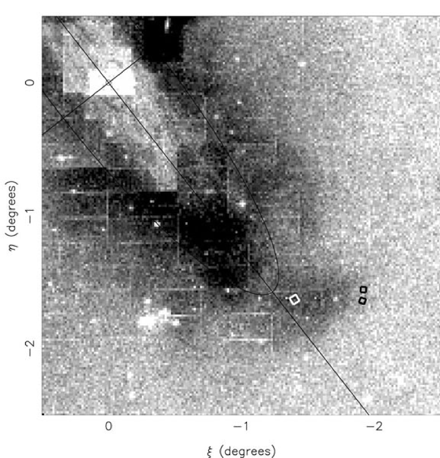
Figure 1.— Surface density plot of individual stars along the south-western major axis in M31. Solid lines show the minor and major axis, and an ellipse representing an inclined disk with $i$ = 77.5^∘ and a radius of 2^∘ ($\approx$ 27 kpc). The G1 clump is seen as an overdensity of stars just outside the ellipse along the major axis at $\xi$ $\sim-1.5$ and $\eta$ $\sim-1.75$. The white box indicates the position of our HST/ACS field. The upper black box shows the position of the HST/WFPC2 field (PID 5464), centered on the G1 globular cluster, studied by Rich et al. (1996). The lower black box shows the position of the HST/WFPC2 field (PID 9099) studied by Rich et al. (2004).

The position of our ACS G1 clump field was selected to coincide with the peak of the stellar overdensity (see Figure 1). The field was observed for one orbit in the F606W filter (broad $V$) and two orbits in the F814W filter ($I$), all within a single visit. Integer pixel dithers were executed between multiple sub-exposures to aid warm pixel and cosmic ray rejection. Final exposure times were 2430 s in F606W and 5150 s in F814W. We note that previous HST studies of this region have been based on fields lying at the very periphery of the stellar overdensity (Rich et al. 1996, 2004).

The images were first processed through the ACS pipeline and then combined per passband using Multidrizzle (Koekemoer et al.  2002) within PyRAF. We used the default mode of Multidrizzle which calculates the offsets between dithered exposures using the information in the image header world coordinate system. We checked the accuracy of this method by measuring the alignment of the individual drizzled frames before the final combine operation. We found images taken in a given filter to be registered to better than 0.1 pixel. We also checked that the centers of stars were not being misidentified as cosmic rays, and no problems were noted. For the final drizzle, we used the Lanczos3 kernel with pixfrac and scale set to unity.

Photometry was obtained using the IRAF implementation of DAOPHOT (Stetson 1987). The stellar density in the G1 field is low enough to allow precise results from aperture photometry alone. An aperture radius of 2 pixels was found to give the best results (i.e. the tightest CMD). PSF-fitting photometry was also carried out in order to reject non-stellar objects such as background galaxies, and cosmic rays which were not previously eliminated. A spatially-invariant PSF was created for each filter using the $\sim$150 brightest stars on the combined images. After PSF-fitting, sources were retained in the final photometry list if their magnitude errors, sharpness and $\chi$ values all lay within 3-sigma of the average value at their magnitude. Final aperture photometry was then re-run on the cleaned star list.

Aperture corrections were derived as follow. The corrections from 2 to 4 pixel aperture radii were found from the average of several tens of bright stars on each frame. No significant variation in the aperture correction over the frame was found. In order to get good signal-to-noise, the aperture correction from 4 to 8 pixels was found using the PSF template star. Finally the photometry was corrected from 8 pixel to ‘infinite’ aperture using the tabulated values given in Table 3 in Sirianni et al. (2005). Table 1 summarises the aperture correction values used. As a further test that there was no systematic variation of the photometry across the ACS field, we produced colour magnitude diagrams in different sub-regions of the chip. We found that these were identical, with no detectable variation in position or colour of the morphological features observed.

The photometry was placed on the Vegamag system using the values given in Table 10 of Sirianni et al. (2005). We adopted a reddening in the G1 clump field of E($B-V$) = 0.06 (Schlegel et al. 1998). The final Vegamag magnitudes used in this paper (referred to as $m_{606}$ and $m_{814}$ throughout) are then

$$m_{\rm fil}=\rm-2.5log(m(2))-C(2-\infty)+zpt-A_{\rm fil},$$

where m(2) is the measured value, in ADU/s, in the 2 pixel radius aperture, and the aperture correction, $C$, zeropoints, $zpt$, and extinction corrections, A_fil, are given in Table 1.

At a few points in the analysis, we require Johnson-Cousins magnitudes (referred to as $V$ and $I$) in order to be able to compare to models in the literature. These are obtained using the calibration presented in Sirianni et al. (2005). The transformation equations have the following form for ($V-I$) $>$ 0.4:

$$\rm V=m_{\rm 606OB}+26.331+0.340(V-I)-0.038(V-I)^{2}$$

$$\rm I=m_{\rm 814OB}+25.496-0.014(V-I)+0.015(V-I)^{2},$$

where m_606OB = $m_{606}$ – 26.398 and m_814OB = $m_{814}$ – 25.501 (i.e. zero point subtracted magnitudes). $V$ and $I$ are obtained by iterating the equation above until convergence is reached ($\sim$ 10 iterations). An initial estimate of ($V-I$) = $m_{606}$ – $m_{814}$ was used. As discussed in Sirianni et al. (2005), errors of a few percent can be introduced by making this transformation.

Completeness tests were carried out separately for each filter. The artificial stars used in the completeness tests were created using the PSFs described above. The completeness value for a given magnitude was calculated by adding approximately 1500 artificial stars with that magnitude to the image, and then running the same photometric pipeline as used for the data (e.g. detection, aperture photometry, PSF fitting and pruning, and final aperture photometry). The final completeness value is then the percentage of the input stars which are recovered. Completeness tests were carried out at a number of magnitudes spanning the entire magnitude range in the data. Figure 2 shows the completeness levels for the $m_{814}$ and $m_{606}$ magnitudes respectively.

	F606W	F814W
aperture correction 2 - 4	–0.22	–0.31
aperture correction 4 - 8	–0.078	–0.087
aperture correction 8 - $\infty$	–0.105	–0.106
zeropoint (Vegamag)	26.398	25.501
extinction correction	0.173	0.117

Table 1Aperture corrections and zeropoints used in photometric calibration

3. The Colour-Magnitude Diagram of the G1 Clump

Figure 3 shows the CMDs of the G1 clump ACS field, which contain a total of 44420 stars. The error bars show average $\pm$1 sigma errors on the magnitudes determined from the artificial star tests. For magnitudes brighter than $m_{814}$_,0 $\sim$ 23.5 ($m_{606}$_,0 $\sim$ 24), the error bars are negligible. The 90% and 50% completeness limits found from the tests are indicated by solid lines.

The main features in the CMD can be summarised as follows:

Figure 2.— Completeness in $m_{814}$ and $m_{606}$ derived from artificial star tests. Dashed lines indicate the 90% and 50% completeness levels.

• A broad, well-populated Red Giant Branch (RGB) of hydrogen-shell burning stars. The width is much larger than can be explained by the photometric errors alone, suggesting a spread in metallicity and/or age. CMDs of the outer regions of M31 have been known for a long time to show metal-rich RGBs with significant dispersion (e.g. Mould & Kristian 1986; Durrell et al. 1994, 2001; Holland et al. 1996), and the RGB in the G1 Clump field is no exception.

• A pronounced Red Clump (RC) of core He burning stars at magnitude $m_{814}$_,0 $\sim$ 24.1 indicating a dominant population of stars with an intermediate age (i.e. 2 – 10 Gyr). There is no obvious extended Horizontal Branch (HB), which suggests the absence of a significant population of truly ancient ($>10$ Gyr) stars. However, note that the faint blue HB expected for an ancient metal-poor population could be masked by the blue plume.

• A Blue Plume (BP) at ($m_{606}$ – $m_{814}$)₀ $\sim$ 0.1 extending from $m_{814}$_,0 $\sim$ 26 to $m_{814}$_,0 $\sim$ 23, which is a possible signature of young main-sequence stars.

• A clump of stars at $m_{814}$_,0 $\sim$ 23.0 and ($m_{606}$ – $m_{814}$)₀ $\sim$ 0.90 which we identify as the Asymptotic Giant Branch (AGB) bump, a feature caused by a temporary slowing down of luminosity increase at the beginning of a star’s AGB phase.

• A low-level overdensity of stars just below the RC at $m_{814}$$\sim$ 24.7 and ($m_{606}$ – $m_{814}$)₀ $\sim$ 0.75. This is identified with the RGB bump, a feature which is caused by the temporary drop in an RGB star’s luminosity when the expanding hydrogen-burning shell reaches the chemical discontinuity left behind by the convective layer during its main sequence phase.

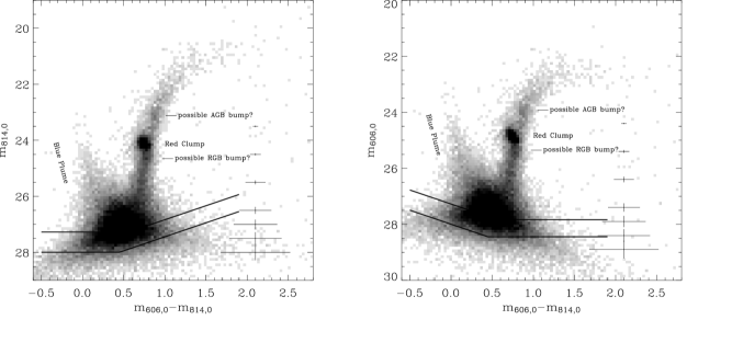
Figure 3.— ($m_{606}$ – $m_{814}$)₀, $m_{814}$_,0 ($left$) and ($m_{606}$ – $m_{814}$)₀, $m_{606}$_,0 ($right$) Hess diagrams (44,420 stars) for our G1 clump field. The solid lines show the 90% and 50% completeness limit determined from artificial star tests. Typical errors along the red giant branch are plotted on the right hand side.

4. Constraining the Age and Metallicity of the G1 Clump

Although our CMD is the deepest yet obtained for this region of M31, it does not reach the level of old main sequence turnoffs. As a result, we are unable to conduct a rigorous study of the full star formation and chemical evolution history of the G1 Clump. Nonetheless, our CMD is of sufficient quality and depth to allow a much more detailed exploration of the stellar populations than has been carried out in previous work. Our adopted approach is to use initial isochrone fitting to guide our choice of model stellar populations and then explore how well different combinations of age and metallicity within this range can reproduce the observed CMD morphology and luminosity function in detail.

Our modeling exploits the Girardi isochrones (Girardi et al. 2000) transformed into the ACS filter bandpasses. Metallicities are calculated assuming [M/H] = log(Z/Z_⊙), [$\alpha$/Fe] = 0 and Z_⊙ = 0.019. The model CMDs used are created using the testpop program from the StarFISH software developed by Harris & Zaristky (2001). In short, testpop creates artificial CMDs based on an input star formation history and data describing observational parameters such as completeness and photometric errors. A detailed description of testpop is given in Harris & Zaritsky (2001). To create the synthetic CMDs discussed below, we have assumed a distance modulus of $(m-M)$ = 24.47 (McConnachie et al. 2005), a binary fraction of 50% and a Salpeter IMF slope of –1.35. The StarFISH software provides two ways to define completeness and errors, either by using an output table from the artifical star tests, or by fitting functions to the results of these tests. We have used the second of these two methods. For the error model, we fit an exponential function to the errors found in the artificial star tests. The completeness is modeled using two separate $arctan$ functions which characterise the completeness function above and below the 50% completeness level.

4.1. The Blue Population in the G1 Clump

4.1.1 The Blue Population as Young Main Sequence Stars

The most striking difference between our CMD and those previously presented for this region (Rich et al. 1996, 2004) is the clear presence of a BP at ($m_{606}$ – $m_{814}$)₀ $\sim$ 0.1 extending from $m_{814}$_,0 $\sim$ 26 to $m_{814}$_,0 $\sim$ 23. In the following, we investigate the BP under the assumption that it is a young population of main-sequence stars.

Figure 4 shows the BP and overlaid Girardi isochrones with [M/H] = –0.4 dex and ages = 250, 650, 1000, and 1800 Myr. The youngest isochrone with age = 250 Myr provides the best fit to the brightest stars, but lies blueward of the main plume, which seems better-described by somewhat older ages. More metal poor isochrones fall further towards the blue and hence fail to reproduce any aspect of the BP. More metal rich isochrones fall further to the red, and could thus possibly be used to fit the redder part of the BP, however no single age and metallicity isochrone can fit the entire BP. This is the first suggestion of an age range – implying extended star formation – in this region of the CMD.

To illustrate this, and to investigate the BP in more detail, we use synthetic CMDs produced with StarFISH. In Figure 5, a model CMD of a population with ages = 250, 650, 1000, and 1800 Myr and [M/H] = –0.4 dex is shown. The four boxes indicated along the BP are used to roughly scale the number of stars in the four age components to the data in the following way: the brightest box only samples stars in the 250 Myr component, the second brightest box sample stars in the 250 and 650 Myr components, etc. Using the brightest box to scale the 250 Myr component provides an estimate of the number of 250 Myr stars in the second box, which can then be used to scale the 650 Myr component, and so on. The total number of stars in the model BP is $\sim$5000, with increasingly more mass in older components (almost 65% of the total mass is in the oldest component).

The resulting model BP is a reasonable match to the data although still slightly too blue. No distinct subgiant branch can be seen for the younger components in the model, but one does appear for the oldest (and most dominant) population at $m_{814}$_,0 $\sim$ 26 and ($m_{606}$ – $m_{814}$)₀ $\sim$ 0.4. In the actual G1 Clump data, the BP merges with the RGB at a slightly fainter magnitude than this, and this may explain why a distinct turnoff is not discernible in the data. Our model of the BP is overly simplistic in that we have used only four ages to model the population. While this has been sufficient to demonstrate that an age range is required to match the observed population, it represents a star formation history consisting of discrete bursts. In reality, the star formation history of the G1 clump region is likely to have varied continuously. Indeed, more sophisticated models which incorporate smaller age bins and extend to ages $>1800$ Myrs produce a smoother BP and the sub-giant branch seen in Figure 5 disappears. However the scaling of such models becomes much more complicated, especially in the region where the BP merges with the RGB, and they are not developed further here.

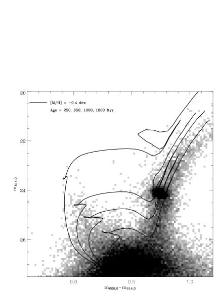
Figure 4.— ($m_{606}$ – $m_{814}$)₀, $m_{814}$_,0 Hess diagram with overlaid Girardi et al. (2000) isochrones with [M/H] = –0.4 dex and ages = 250, 650, 1000, and 1800 Myr.

The model in Figure 5 also predicts the CMD location of the evolved counterparts to such a young population. Evolved stars from the two younger age components are expected to fall on the blue side of the RGB (i.e. at ($m_{606}$ – $m_{814}$)₀ $\leq$ 0.75 and $m_{814}$_,0 $\leq$ 23 ), extending upwards from the observed RC. This feature is called a blue loop (see Gallart 1998 and references within). Although we do not observe a well-defined blue loop population in the G1 Clump CMD, we do see a number of stars in this region and their number is in good agreement with our simple model predictions.

For the two older populations, ages = 1000 and 1800 Myr, the evolved stars are superimposed on the RGB and RC. The possible influence this will have on the interpretation of these features will be further discussed in the next section. We note, however, that the number of stars in our BP model is only $\approx 10\%$ of the total number of observed stars in the G1 clump field and that the bulk of these stars lie in the BP itself.

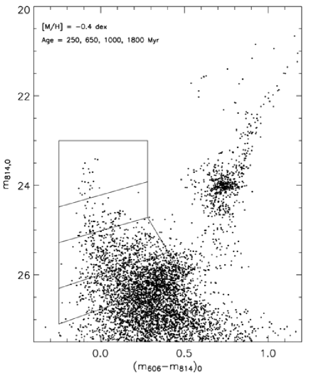
Figure 5.— ($m_{606}$ – $m_{814}$)₀, $m_{814}$_,0 synthetic CMD showing the model of the blue plume ([M/H] = –0.4 dex and ages = 250, 650, 1000, and 1800 Myr).

4.1.2 The Blue Population as Blue Straggler Stars

An alternative interpretation of the BP is that it represents a population of blue straggler stars. CMDs of globular clusters and nearby dwarf galaxies often show a BP similar to the one we observe in the G1 clump. In globular clusters, where there is no recent star formation, the BP is identified with rejuvenated blue straggler stars, created either by stellar collisions or by mass transfer in primordial binaries (Davies et al. 2004). In more complex stellar systems, such as dwarf spheroidal galaxies, the nature of the BP is less clear. It has been attributed both to blue stragglers (e.g. in Ursa Minor, Carrera et al. 2002) as well as young and intermediate age populations (e.g. in Draco, Aparicio et al. 2001).

In sparsely-populated stellar environments, such as the Milky Way halo, the important mechanism for blue straggler formation is believed to be mass transfer in primordial binaries (Carney et al. 2001). In this scenario, one expects the blue stragglers to have masses lower than twice the main-sequence turn-off mass ($M_{MSTO}$) of the underlying population from which they have formed. However, in dense stellar environments (i.e. globular clusters) theorists predict that binary-binary collisions may occasionally produce blue stragglers which are more massive than twice the turn-off mass (Fregeau et al. 2004), but examples of this have yet to be observed.

The two youngest isochrones overlaid in Figure 4 (ages = 250 and 650 Myr) have main-sequence turn-off masses, $M_{MSTO}$ $\sim$ 3.2 and 2.1 M_⊙. A significant fraction of the stars on the BP thus appear to have masses $\geq$ 2 M_⊙ and reaching as high as 3 M_⊙. To explain such stars as blue stragglers formed via mass transfer, we would require a progenitor population of stars with $M_{MSTO}\gtrsim 1.5$ M_⊙. Such a population would have ages of $\sim$ 2–3 Gyr . In Section 4.2, we will show that the G1 clump very likely contains such a population. We therefore cannot rule out blue straggler stars as contributors to the BP.

We can further test the likelihood of a blue straggler contribution to the BP by calculating the blue straggler specific frequency, defined as the number of blue straggler stars compared to the number of RC stars, $S_{(BS)}$ = $N_{BS}$/$N_{RC}$. We calculate $N_{RC}$ by counting all stars on the RGB within 24.35 $<$ $m_{814}$_,0 $<$ 23.85, then correcting for the estimated number of RGB stars within this same region by measuring the number of stars above and below the RC. $N_{BS}$ was calculated by selecting all stars with $m_{814}$_,0 $<$ 26 and ($m_{606}$ – $m_{814}$)₀ $<$ 0.5. Using these definitions for $N_{BS}$ and $N_{RC}$, we find $S_{(BS)}$ = 1.7 for the G1 clump. This value can be compared to the values found for globular clusters ($S_{(BS)}$ $\leq$ 2) and for the MW halo field population, $S_{(BS)}$ $\sim$ 4 (Preston & Sneden 2000, and references within). While the specific frequency of blue straggler stars in the G1 clump is slightly lower than that seen elsewhere, the discrepancy is not so significant that we can rule out this hypothesis.

The blue straggler interpretation of the G1 Clump’s BP population thus remains viable though we do not favour it here. In particular, we note that the CMDs of other stellar overdensities in the outskirts of M31 do not show such strong BP populations as the G1 Clump (Ferguson et al. 2005), even though many of these other fields have similar or greater stellar densities. This argues against the idea that the BP population is primarily composed of blue straggler stars, since such stars should be expected in similar amounts in all fields. Furthermore, as we will argue later, the existence of a genuinely young population is consistent with the location of the G1 Clump field within M31’s HI disk and our derived metallicity for the population is consistent with that expected from extrapolation of M31’s chemical abundance gradient.

4.2. The Old and Intermediate-Age Populations of the G1 Clump

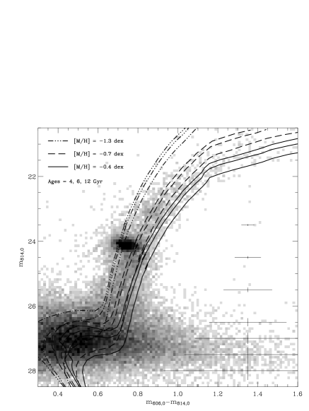
Figure 6.— ($m_{606}$ – $m_{814}$)₀, $m_{814}$_,0 Hess diagram of the red populations with overlaid Girardi et al. (2000) isochrones with [M/H]= –1.3, –0.7, and –0.4 dex and ages = 4, 6 and 12 Gyr.

We can obtain constraints on the age and metallicity of old and intermediate-age populations of stars in the G1 Clump from analysis of the locus and width of the RGB in conjunction with the position and morphology of the RC (e.g. Ferguson & Johnson 2001). In addition, the position of the AGB and the RGB bumps can be used to provide consistency checks on our best-fitting models (e.g. Alves & Sarajedini 1999) provided that these low-level features can be correctly identified in the CMD.

4.2.1 Comparison to Theoretical Isochrones

As a first step, we compare the G1 Clump’s RGB to the Girardi isochrones calculated for a range of ages and metallicities. Figure 6 shows the CMD overlaid with isochrones of ages = 4, 6, and 12 Gyr and metallicities [M/H] = –1.3, –0.7, and –0.4 dex for each age.

The metal poor isochrones ([M/H] = –1.3) all fall on the blue side of the RGB, and the curvature at the bright end is clearly not correct. The more metal rich isochrones provide better matches, although no single isochrone appears to fit the RGB along its whole length. At the faint end, the RGB locus is best matched by an intermediate age and metallicity model (i.e. 4–6 Gyr and [M/H] $\sim$ –0.7 dex), whereas at the bright end, more metal rich isochrones with [M/H] $\sim$ –0.4 dex do equally well.

Figure 7.— Girardi & Salari (2001) models of RC behavior as a function of age and metallicity. Thick solid lines indicate the position of the red clump in the G1 Clump field.

Figure 8.— Luminosity function in $m_{606}$_,0 (top) and $m_{814}$_,0 (bottom). Solid lines show Gaussian fits to the red clumps.

The RGB is much wider than can be explained by the photometric errors, especially above the RC, suggesting that it cannot be explained by a single age and metallicity population. An estimate of the maximum possible metallicity spread can be found if we assume a single age population. From Figure 6, the metallicity spread required to explain the full width of the RGB is $\gtrsim$ 0.6 dex spanning from $\lesssim$ –1 dex to $\gtrsim$ –0.4 dex. On the other hand, if we assume a single metallicity, we find that the required age spread needed to explain the full width of the RGB must be greater than the the entire age span of the overlaid isochrones in Figure 6 (i.e. $\gtrsim 8$Gyr).

As is well known, it is impossible to distinguish between a spread in metallicity and a spread in age by looking solely at the RGB. Fortunately, our CMD shows several additional features which can be used to break the age-metallicity degeneracy, the most prominent being the RC.

4.2.2 Red Clump Models

Figure 7 shows models from Girardi & Salaris (2001) which illustrate the RC behavior as a function of age and metallicity. For ages older than $\sim$ 2 Gyr, the mean colour of the RC has a strong dependence on metallicity but almost no dependence on age. On the other hand, for a given metallicity, the mean magnitude of the RC depends strongly on age, so that an older population is expected to have a fainter RC than a younger one. Together the mean magnitude and colour of the RC can provide insight into the age and metallicity mix of the constituent stellar populations (e.g. Ferguson & Johnson 2001; Rejkuba et al. 2005).

The position of the RC in the G1 Clump CMD was found by fitting a Gaussian to the luminosity function in $m_{606}$_,0 and $m_{814}$_,0, as shown in Figure 8. Following Paczynski & Stanek (1998), a 5-parameter Gaussian was used with the two additional parameters representing a constant $y$-offset and linear slope term. The centroids of the Gaussians are: $m_{606}$_,0 = 24.871 $\pm$ 0.004 and $m_{814}$_,0 = 24.125 $\pm$ 0.004, which gives ($m_{606}$ – $m_{814}$)₀ = 0.746 $\pm$ 0.006. Using the transformations from the ACS photometric system to $V$ and $I$ described in Section 2, these values translate into $M_{I,\rm{RC}}=-0.349$, $M_{V,\rm{RC}}=0.631$, and $(V-I)_{RC}=0.980$, using ($m-M$)$=24.47$. Comparing these values with the models in Figure 7 (solid lines), we infer a stellar population with a mean metallicity [M/H] $\sim$ –0.4 dex and intermediate age $\sim$ 3.5 Gyr. These values are broadly consistent with those found earlier from isochrone comparisons. We note there is some degree of degeneracy in the models in Figure 7; our RC properties could also be consistent with a $\sim$1-2 Gyr solar metallicity population. This will be further commented on later in this section. Furthermore, uncertainties in the distance modulus could change the mean age derived by this relatively crude method by several Gyr.

The analysis above provides only a mean age and metallicity of the population, whilst in reality there could be several different populations contributing to the CMD. We now proceed to use the detailed morphology of the RC to place contraints on the mix of populations that might be present. Figure 9 shows a comparison between the observed RC and the RC of various synthetic populations spanning a range of ages and metallicities. For both the real data and the synthetic models, we show the CMD, luminosity function, and colour distribution for the RC region. The results from the data are shown in Figure 9A and overlaid on each of the models to aid with the comparison. The number of stars in the RC region of the model populations is adjusted to match the real RC to within a few percent.

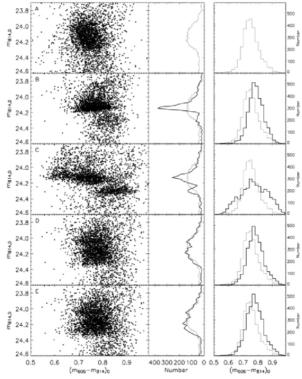
Figure 9.— Synthetic CMDs (left), luminosity functions (center), and colour distributions (right) showing observed (light) and model (bold) distributions. (A) Shows the observed red clump of the G1 clump field. (B) shows a single age and metallicity model (age = 4 Gyr and [M/H] = –0.4 dex). (C) Shows a model with a significant metallicity spread (age = 4 Gyr, [M/H] = –1.3, –0.7, –0.4, and 0.0 dex). (D) Shows a model with a significant age spread and a single metallicity (age = 2, 4, 6, 8, and 10 Gyr, [M/H] = –0.4 dex). (E) Shows a model with a significant age spread and a small spread in metallicity (age = 2, 4, 6, 8, and 10 Gyr, [M/H] = –0.4 dex, and age = 6, 8, and 10 Gyr for M/H] = –0.7 dex).

The first model (Figure 9B) is of a single age and metallicity population similar to the mean properties derived above (age = 4 Gyr and [M/H] = –0.4 dex). The model RC morphology is clearly different to the data – the vertical extent of the RC model is much too small and slightly too red; the corresponding luminosity function emphasizes this even further. This comparison indicates that the observed RC cannot be fit by a single age and metallicity population.

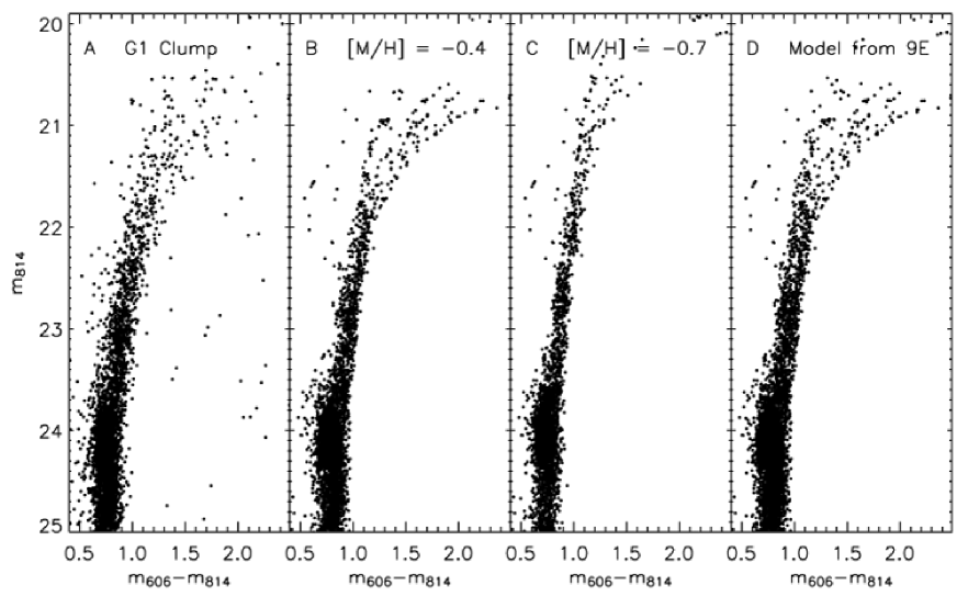
Figure 10.— Synthetic ($m_{606}$ – $m_{814}$)₀, $m_{814}$_,0 CMDs showing the red giant branch. (A) Shows the red giant branch of the G1 clump field. (B) Shows a model with a single metallicity and a large age spread (age = 2, 4, 6, 8, and 10 Gyr, [M/H] = –0.4 dex). (C) Shows the same as (B) but with lower metallicity ([M/H] = –0.7 dex). (D) shows the same model as in Figure 9E. The blue plume model from Figure 5 is overlaid on the models in (B), (C) and (D).

The model in Figure 9C has a single age but a spread in metallicity (age = 4 Gyr, [M/H] = –1.3, –0.7, –0.4, and 0.0 dex). This model produces a vertical extent which is similar to the data, but the morphology is clearly incorrect. In addition to there being two distinct RC sequences in this model, the overall colour spread is much too large. In fact, it turns out that any significant population of stars with a metallicity higher than $\sim$ –0.2 dex or lower than $\sim$ –0.7 dex results in a RC with a colour spread that is larger than observed. On the other hand, restricting the metallicity spread to be $\sim$ –0.2 to $\sim$ –0.7 dex results in a RC with a vertical extent which is much too small compared to the observed spread in Figure 9A. This comparison indicates that even a single age population with a range in metallicity fails to reproduce the observations.

Figure 9D shows a model with a pure age spread (age = 2, 4, 6, 8, and 10 Gyr) and a single metallicity ([M/H] = –0.4 dex). The scaling of each age component was done to fit the luminosity function of the data in a similar way to the scaling of the BP model. The model RC provides a good match to the observations in terms of both general morphology as well as vertical extent. The colour of the model RC is slightly too red ($\sim$0.02 mag) indicating that the metallicity of the model is slightly too metal-rich, which is in good agreement with Figure 7. The metallicities of our models are limited by what is available in the Girardi isochrone set, so we are not able to model the effects of small metallicity variations. Our modelling is not sophisticated enough to precisely constrain the age of the stellar population and there is some uncertainty in the oldest ages present. For example, almost identical RC morphologies are obtained for a slightly higher metallicity and a lower maximum age, or for slightly lower metallicities and a higher maximum age. Nonetheless, our synthetic modeling of the RC demonstrates that an age spread is required to reproduce the observations. This is further strengthened by a two-sided Kolmogorov-Smirnov test which yields a probability of $\sim$ 40% that our model in Figure 9D and the data are identical.

In order to test the effects of introducing a small metallicity spread, Figure 9E shows the same model as in Figure 9D but with the addition of a more metal-poor population in the older age bins (age = 6, 8 and 10 for [M/H] = –0.7 dex). The metal-poor component contains 25% of the total mass in the model. We did not add stars in the younger age bins since they would produce an RGB which is significantly bluer than the observed RGB at the bright end (see Sect. 4.2.3 and Figure 10 ). As discussed above, such a metallicity range is still within that allowed by the colour width of the RC. The model RC is marginally wider in colour than the observed RC at the faint end and the agreement with the luminosity function is less good than before but this may be partially due to the discrete ages and metallicities used in our model. It is possible that adopting a smooth age-metallicity relation across this metallicity range could provide an equally good match to the data as the model in Figure 9D. In summary, although we cannot exclude a small metallicity range within the population, we have demonstrated that it is not required to model the observations of the red clump.

As noted earlier, we expect the evolved counterpart of any young BP component to be superimposed on the RC (see Figures 5 and 7). A more realistic model of the BP would have continuous star formation, instead of discrete ages, and since the change of the RC luminosity is a very strong function of age for ages less than $\sim$2 Gyr, the result would be that the stars from the younger population would be smeared out over $\sim$0.8 magnitudes which is roughly the same vertical width as the old RC. We therefore believe that the presence of a very young ($<2$ Gyr) component in the RC would not significantly alter the conclusion derived from the above analysis. It is however possible that the small overdensity of stars below the RC that we identify with the RGB bump (see next section) could be somewhat contaminated by evolved stars in the young population or a mix of both.

Also, we argued previously that if a population of age 2–3 Gyr was present, the BP could be interpreted as blue stragglers rather than a young population. The modelling above shows that such a population is required to explain the morphology of the RC and thus that this scenario for the blue population cannot definitively be excluded.

4.2.3 Red Giant Branch Models

The modeling presented in the previous section demonstrates that a population with a large age spread and with either a single metallicity, or a small metallicity spread, can reproduce the overall properties of the RC. We next proceed to investigate whether the models explored in the red clump modelling can also reproduce the appearance of the RGB. Figure 10 shows a comparison between the observed RGB and three different metallicity models, two with a single metallicity and a large age spread, and one with a large age spread and small metallicity spread.

In Figure 10A, we show the observed G1 Clump RGB. Figure 10B and C show synthetic models of the RGB constructed with pure age spreads (age = 2, 4, 6, 8, and 10 Gyr for [M/H] = –0.4 and [M/H] = –0.7 dex, respectively). These metallicities were found to be the best matches in the RC modelling. In addition, our models include the contribution from the BP model shown in Figure 5 (age$<2$ Gyr). As before, we find that the more metal-rich model ([M/H] = –0.4 dex) in Figure 10B shows a closer resemblance to the data. In particular, the youngest stars in the metal-poor model form a much straighter and bluer RGB at the bright end as compared to the observed CMD. Furthermore, the [M/H] = –0.4 dex model shown here is a much better match to the lower part of the RGB than were the metal-rich isochrones overlaid in Figure 6. This is due to the younger age components now present in the model, which shift the RGB colour towards the blue, particularly at the fainter end. At brighter magnitudes, the evolved counterparts of the BP population scatter blueward of the main RGB. A BP model with a continuous star formation history would better populate the blue side of the entire RGB, similar to what is seen in the data. The single metallicity model in Figure 10B is slightly narrower than the data in the magnitude range 22.5 $<$ $m_{814}$$<$ 23.5. Figure 10D shows the RGB of the model with a large age spread and small metallicity spread introduced in Figure 9E. While the RC in this model did not look as good as in the single metallicity model, the RGB width in this model is more similar to the data, although the difference is small.

We conclude that while the model with [M/H] = –0.4 dex and an age spread of 0.25–10 Gyr can adequately reproduce the overall width and shape of the observed RGB, a small metallicity spread, such as that shown in Figure 9E, could also be present.

4.2.4 The RGB and AGB Bumps

In addition to the RC, two other overdensities of stars can be seen along the RGB at $m_{814}$_,0 $\sim$23.0 (($m_{606}$ – $m_{814}$)₀ $\sim$0.9) and just below the RC at $m_{814}$_,0 $\sim$24.7 (($m_{606}$ – $m_{814}$)₀ $\sim$0.75) and merging with the RC. Both features are indicated in Figure 3 and Figure 8. We identify these features with the AGB and RGB bump respectively. The brightnesses of these features are expected to vary with age and metallicity as shown in models presented by Alves & Sarajedini (1999). According to these models, the fact that the AGB and RGB bump straddle the RC in our data is a strong indication of metallicities above $\sim$ –0.7 dex. For a metallicity of [M/H] = –0.4 dex (the highest metallicity they examine), interpolating between the age bins given in their Table 2 leads one to expect $\Delta M_{V,\rm{RGBbump-RC}}$ $\sim$0.4 mag for an 8 Gyr population, and $\sim-0.1$ mag for a 3 Gyr one. Using the calibrations from Sirianni et al. and the distance modulus as before, we find the observed magnitude difference between the RGB bump and the RC to be $\Delta M_{V,\rm{RGBbump-RC}}$ $\sim$0.4 mag. Thus, the position of the RGB bump is in broad agreement with the the constraints derived earlier on the age and metallicity range of the population.

Alves & Sarajedini (1999) also predict the difference between the AGB bump and the RC, $\Delta M_{V,\rm{AGBbump-RC}}$. For [M/H] = –0.4 dex, they show that this value is expected to be $\sim$ -0.8 magnitudes regardless of age. Since the RC luminosity varies with age, this implies that the peak of the AGB bump should be 0.8 magnitudes above the peak of the RC and should have a comparable vertical spread. The presence of a low-level overdensity of stars comparable in luminosity extent to the RC at $m_{814}$_,0 $\sim$23, corresponding to $\Delta V_{\rm AGBbump-RC}$ $\sim$ -0.7, is thus consistent with the expected location of the AGB bump.

4.3. The Final G1 Clump Model

Age	Mass	Fraction of Total Mass
(Gyr)	(103 $\times$ M⊙)	%
0.250	12.25	0.2
0.650	25.00	0.5
1.0	45.00	0.8
1.8	225.0	4.2
2.0	300.0	5.5
4.0	800.0	14.8
6.0	1200	22.2
8.0	1400	25.9
10.0	1400	25.9

Table 2Stellar populations in our final model of the G1 clump.

Our final model of the G1 clump field is a combination of the BP model in Figure 4 and the RGB model with a pure age spread shown in Figure 9D and in Figure 10B. This model contains populations of ages 0.25–10 Gyr at a uniform metallicity of [M/H]$=-0.4$. We stress again that our aim has not been to produce a high precision star formation history of the G1 Clump, but rather to come up with a simple model that can reproduce the detailed morphology of the CMD and thus yield insight into the nature of the constituent populations. We have previously commented on the fact that a small metallicity range could be present and still be consistent with the observed CMD. Likewise, we have no way to constrain the presence of an additional component with ages $>10$ Gyr. Figure 11 shows that our model CMD is in very good qualitative and quantitative agreement with the observations. Table 2 shows the ages and masses in each component of the model; the bulk of the stars have ages $>6$ Gyr, however $\approx 10$% of the mass is contained in a population younger than 2 Gyr.

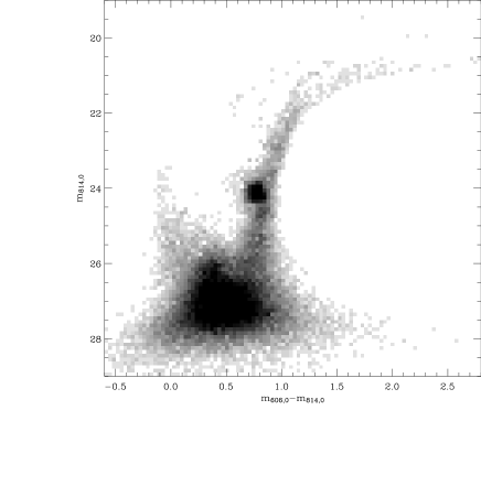
Figure 11.— ($m_{606}$ – $m_{814}$)₀, $m_{814}$_,0 Hess diagram of the final model of G1 clump field (45,085 stars). The model is a combination of the blue plume model in Figure 4 and the red giant branch model with a pure age spread shown in Figure 9D and in Figure 10B.

Figure 12 shows the corresponding LF for the model compared to that observed for the G1 Clump. The model LF is in excellent agreement with the data along the entire RGB. A small deviation can be seen at $m_{814}$_,0 $\sim$ 23 where the model fails to reproduce in detail the AGB bump. When more stars are added into the model, an AGB bump is produced at the correct position. The problem therefore is that the model AGB bump is weaker than the observed bump. This problem was also seen in the modelling of Gallart (1998)

For simplicity the analysis presented here has assumed no $\alpha$-enhancement. The effect of $\alpha$-enhancement has however been thoroughly investigated using the isochrones described in Salasnich et al. (2000). Introducing $\alpha$-enhancement has the effect of increasing the derived metallicity from [M/H] $\sim$–0.4 (non $\alpha$-enhanced) to [M/H] $\sim$0.0 ($\alpha$-enhanced), but does not alter the derived age spread.

5. Discussion and Conclusions

Our deep CMD analysis of the G1 Clump suggests a constituent population characterised by a relatively high mean metallicity ([M/H]$\sim-0.4$) and an age range of at least 0.25–10 Gyr. In our model, the bulk of the stellar mass is of age $>6$ Gyr. Such a population represents a continuous, albeit declining, star formation history over at least 10 Gyr with only a mild amount of associated chemical evolution. The presence of a young-to-intermediate age component in the vicinity of G1 was suggested in the WFPC2 studies of Rich et al. (2004). Our deeper ACS CMD has provided conclusive evidence for this population and quantified its significance.

The metallicity we derive for the bulk population in the G1 clump is significantly higher than values found in earlier studies. Rich et al. (2004) find a metallicity of [Fe/H] $\sim$ –0.7 dex, which can be taken as [M/H] on the assumption of [$\alpha$/Fe]$=0$. We believe this difference can largely be explained by the presence of an age range within the G1 clump field. If the metallicity is derived assuming a uniformly old stellar population (i.e. by comparison with Galactic globular cluster fiducials or old isochrones), a lower metallicity will be found. This is illustrated in Figure 6 where it can be seen that a change in age from 12 Gyr to 4 Gyr will change the derived metallicity by $\sim$ 0.3 dex, or roughly the same difference between our value and that of Rich et al. (2004).

Figure 12.— Luminosity function in $m_{814}$_,0. The thin line shows the completeness corrected G1 clump luminosity function for the red giant branch. The thick line shows the corresponding luminosity function for our final model shown in Figure 11. Poissonian errors for each bin are shown on the model luminosity function

The BP model in Figure 5 can be used to estimate the total mass of the young population in the G1 Clump field. Assuming a Salpeter IMF with the exponent = –1.35 and mass cut-off = 0.1 M_⊙, the total mass of our BP population in Figure 5 is approximately 3 $\times$ 10⁵ M_⊙. The 1800 Myr component comprises $\sim$65% of the total mass. This translates to an average star formation rate of approximately 10^-4 M_⊙/yr over the last 1.8 Gyr.

5.1. The G1 Clump as the Remnant of an Accreted Dwarf Galaxy

The morphology of the G1 clump – i.e. an irregular lump distinct from the main disk (see Figure 1) – suggests it could be the remnant of an accreted dwarf galaxy. Recent studies of RGB kinematics in this region have shown the G1 Clump stars to have radial velocities similar but not identical to those of the rotating HI disk in M31 (Reitzel et al. 2004; Ibata et al. 2005). Although this fact has been used to argue against the idea that the G1 Clump is an accreted dwarf, it is possible that some satellites could be accreted on prograde coplanar orbits. Indeed, some argue that the stellar overdensity seen in the Milky Way towards Canis Major may be an example of such an accretion event (e.g. Martin et al. 2004).

It is therefore worthwhile investigating whether the stellar populations of the G1 Clump could be consistent with a low mass satellite. At first glance, the G1 clump appears rather different to present-day dwarf spheroidal galaxies around the Milky Way and M31, most of which show evidence for dominant old and metal-poor populations (see e.g. Dolphin et al. 2005; Da Costa et al. 2002). The estimated absolute magnitude of the G1 clump is $M_{V}$ $\simeq$ –12.6 (Ferguson et al. 2002). Local group dwarfs of this magnitude typically have –2 $<$ [Fe/H] $<$ –1.5 (Mateo 1998), much more metal-poor than the G1 clump for which we find metallicity [M/H] $\sim$ –0.4 dex.

There are, however, a few examples of dSph galaxies which contain both young-to-intermediate age stars as well as stars with moderate metallicities. One of these is the Fornax dwarf which contains a stellar population of mean age 5.4 Gyr (including stars as young as 0.2 Gyr) and with metallicities reaching to almost solar (e.g. Savianne et al. 2000; Tolstoy et al. 2006). The other system is the Sagittarius dwarf galaxy, which the Milky Way is currently in the process of accreting. Analysis of the stellar content in the core of this galaxy reveals a dominant population of age $\sim 6$ Gyr (but lacking any very young stars) and metallicity [M/H]$=-0.5$ (e.g. Bellazzini et al. 1999; Monaco et al. 2005). In spite of the similarities in stellar content, the G1 Clump remains distinct from these systems in terms of its size and surface brightness. At $\sim 10$ kpc, it is many times larger than the core diameters of either Fornax or Sagittarius and roughly 4 magnitudes fainter in peak surface brightness. It thus does not easily fit into the sequence of properties which characterize known dwarf galaxies. An additional argument against the dwarf galaxy hypothesis has been raised by Ibata et al. (2005). They point out that the extent ($\sim 10$ kpc) and velocity dispersion of 30 km/s of the G1 Clump would require a very considerable associated dark mass ($\sim 10^{9}$ M_⊙) in order to be bound. Although we cannot completely exclude this hypothesis with existing data, we conclude that the G1 Clump is unlikely to be an accreted dwarf galaxy.

5.2. The G1 Clump as Perturbed Outer Disk

Another hypothesis for the G1 Clump is that it is a perturbation of the M31 outer disk. Our analysis of stellar populations in the G1 Clump supports this idea on several grounds. First of all, we have demonstrated that the G1 Clump has experienced continuous low-level star formation for most of the last 10 Gyr. This implies a constant supply of gas, consistent with a location in the outer disk of M31. Indeed, Carignan et al. (2006) have shown that M31’s HI disk extends out to at least 35 kpc, well beyond the location of the G1 Clump. The recent average star formation rate of 10^-4 M_⊙/yr compares favourably with that determined for a location at 24 kpc in the outer disk by Williams (2002)(see his Figure 5(a)). In addition, Williams (2002) finds that the outer disk is characterised by a declining star formation rate, consistent with what we have found for the G1 Clump.

Further support for this picture comes from comparing the metallicity of the M31 gas disk with the metallicity of stars in the G1 Clump. The mean metallicity inferred for the G1 Clump, [M/H]$\sim-0.4$ dex, is rather high compared to that typically found in the outer regions of present-day gas disks (e.g. Ferguson et al. 1998). At face value, this might suggest that the G1 Clump cannot have formed from the gas disk in M31. M31 is unusual, however, in having a high mean gas-phase metallicity and a rather flat gradient (e.g. Trundle et al. 2002). At a radius of 26 kpc, the mean oxygen abundance in the disk as determined from HII regions is 40% solar (Ferguson & Urquhart, in preparation). In order to compare the gas-phase [O/H] and the stellar [Fe/H] abundances, we need to a adopt a value for [O/Fe]. Trundle et al. (2002) have compiled [O/Fe] and [$\alpha$/Fe] for supergiant stars in M31 and find that, within the errors, these values are consistent with being zero across the disk. This implies that [M/H]$=$[Fe/H]$\sim$[O/H]$\sim-0.4$ in the outer disk, and hence that stellar metallicity of the G1 Clump is in excellent agreement with the extrapolation of the M31 disk abundance gradient. While it may not strictly be correct to compare the present-day metallicity of the gas disk with that of stars which formed several Gyr ago, the low star formation rate inferred for the G1 Clump implies that, in the absence of gas flows, little chemical evolution will have taken place in this region, even over long periods. This is supported by the small spread in metallicities inferred from our modelling. We note that the high mean metallicity inferred for this region indicates a significant amount of pre-enrichment before the onset of star formation.

Finally, the overall morphology of the G1 Clump shows some similarities (e.g. RGB and RC morphology) to several other fields that lie at large radius along the major axis in M31 (e.g. Ferguson & Johnson 2001; Ferguson et al. 2005) suggesting that all may sample the same structure. Although the strength of the BP is observed to vary between some of these fields, this may simply reflect local variations in the recent star formation rate. For example, the field observed by Ferguson & Johnson (2001) shows a fainter and sparser BP than the G1 Clump field despite lying at a similar distance along the major axis. On the other hand, the Ferguson & Johnson (2001) field lies along the north-eastern major axis in a region where the gas disk severely warps away from the disk plane. As a result, the recent star formation history of this field may well be different from outer disk fields which lie within the main gas disk. On the other hand, the fact that the old and intermediate-age populations in these two fields share similar properties may provide further evidence that the outer regions of the M31 disk have been in place for a significant time, contrary to some theoretical expectations (e.g. Abadi et al. 2003).

If the G1 Clump does represent the outer disk, we require an explanation for its appearance as a distinct overdensity detached from the main body of M31. N-body simulations indicate that the outer regions of disks can suffer significant damage during minor mergers (e.g. Quinn et al. 1993; Walker et al. 1996). In these simulations, the final disk possesses distinct lumpiness at large radius, consisting of stars which existed in the initial stellar disk as well as stars stripped off the accreted satellite. Another possible scenario is a large merger, similar to that studied by Springel & Hernquist (2005). They show that the remnant of a major merger between similar-sized gas disks could still retain some disk structure. In this scenario, the outer disk will consist of stars formed after the merger in the resettled gas disk. The oldest stars in the outer disk would therefore date the merger event. In the case of the G1 clump, we have shown the oldest stars are at least 8-10 Gyr and hence any significant merger of this sort must have happened a long time ago. The existence of copious substructure in the outskirts of M31 strongly supports the idea M31 has experienced at least one significant accretion event (Ferguson et al. 2002) and hence the hypothesis that the G1 Clump represents torn off disk appears viable. Given the stellar population constraints derived here and the kinematical constraints derived elsewhere (Reitzel et al. 2004; Ibata et al. 2005), we strongly favour this hypothesis for the origin of the G1 Clump.

References

- (1) Abadi, M. G., Navarro, J. F., Steinmetz, M., & Eke, V. R. 2003, ApJ, 597, 21
- (2) Alves, D. R. & Sarajedini, A. 1999, ApJ, 511, 225
- (3) Aparicio, A., Carrera, R., & Martínez-Delgado, D. 2001, AJ, 122, 2524
- (4) Bellazzini, M., Ferraro, F. R., & Buonanno, R. 1999, MNRAS, 307, 619
- (5) Bellazzini, M., Cacciari, C., Federici, L., Fusi Pecci, F., & Rich, M. 2003, A&A, 405, 867
- (6) Brown, T. M., Ferguson, H. C., Smith, E., Kimble, R. A., Sweigart, A. V., Renzini, A., Rich, R. M., & VandenBerg, D. A. 2003 ApJ, 592, 17
- (7) Brown, T. M., Smith, E., Guhathakurta, P., Rich, R. M., Ferguson, H. C., Renzini, A., Sweigart, A. V., & Kimble, R. A. 2006, ApJ, 636, L89
- (8) Bullock, J. S., & Johnston, K. V. 2005 ApJ, 635, 931
- (9) Carney, B. W., Latham, D. W., Laird, J. B., Grant, C. E., & Morse, J. A. 2001, AJ, 122, 3419
- (10) Carrera, R., Aparicio, A., Martínez-Delgado, D., & Alonso-García, J. 2002, AJ, 123, 3199
- Carignan et al. (2006) Carignan, C., Chemin, L., Huchtmeier, W. K., & Lockman, F. J. 2006, ApJ, 641, L109
- (12) Chapman, S. C., Ibata, R., Lewis, G. F., Ferguson, A. M. N., Irwin, M., McConnachie, A., & Tanvir, N. 2006, ApJ, in press (astro-ph/0602604)
- (13) Cohen, J. G., Matthews, K., & Cameron, P. B. 2005, ApJ, 634, L45
- (14) Da Costa, G. S., Armandroff, T. E., & Caldwell, N. 2002, AJ, 124, 332
- (15) Davies, M. B., Piotto, G., & de Angeli, F. 2004, MNRAS, 349, 129
- (16) Dolphin, A. E., Weisz, D. R., Skillman, E. D., & Holtzman, J. A. 2005, preprint (astro-ph/0506430)
- (17) Durrell, P. R., Harris, W. E., & Pritchet, C. J. 1994, AJ, 108, 2114
- (18) Durrell, P. R., Harris, W. E., & Pritchet, C. J. 2001, AJ, 121, 2557
- (19) Ferguson, A. M. N., Gallagher, J. S., & Wyse, R. F. G. 1998, AJ, 116, 673
- (20) Ferguson, A. M. N., & Johnson, R. A. 2001, ApJ, 559, L13
- (21) Ferguson, A. M. N., Irwin, M. J., Ibata, R. A., Lewis, G. F., & Tanvir, N. R. 2002, AJ, 124, 1452
- (22) Ferguson, A. M. N., Johnson, R. A., Faria, D. C., Irwin, M. J., Ibata, R. A., Johnston, K. V., Lewis, G. F., & Tanvir, N. R. 2005, ApJ, 622, 109
- (23) Fregeau, J. M., Cheung, P., Portegies Zwart, S. F., & Rasio, F. A. 2004, MNRAS, 352, 1
- (24) Fusi Pecci, F., Bellazzini, M., Buzzoni, A., De Simone, E., Federici, L., & Galleti, S. 2005, AJ, 130, 554
- (25) Gallart, C. 1998, ApJ, 495, 43
- (26) Girardi, L., Bressan, A., Bertelli, G., & Chiosi, C. 2000, A&AS, 141, 371
- (27) Girardi, L. & Salaris, M. 2001, MNRAS, 323, 109
- (28) Harris, J. & Zaritsky, D. 2001, ApJS, 136, 25
- (29) Holland, S., Fahlman, G. G., & Richer, H. B. 1996, AJ, 112, 1035
- (30) Huxor, A. P., Tanvir, N. R., Irwin, M. J., Ibata, R., Collett, J. L., Ferguson, A. M. N., Bridges, T., & Lewis, G. F. 2005, MNRAS, 360, 1007
- (31) Ibata, R., Irwin, M., Lewis, G., Ferguson, A. M. N., & Tanvir, N. 2001, Nature, 412, 49
- (32) Ibata, R., Chapman, S., Ferguson, A. M. N., Lewis, G., Irwin, M., & Tanvir, N. 2005, ApJ, 634, 287
- (33) Irwin, M. J., Ferguson, A. M. N., Ibata, R. A., Lewis, G. F., & Tanvir, N. R. 2005, ApJ, 628, 105
- (34) Juric, M., et al. 2005, preprint (astro-ph/0510520)
- (35) Kalirai, J.S., Gilbert, K.M., Guhathakurta, P., Majewski, S.R., Ostheimer, J.C., Rich, R.M., Cooper, M.C., Reitzel, D.B., & Patterson, R.J. 2006, AJ, 648, 389
- (36) Koekemoer, A. M., Fruchter, A. S., Hook, R., & Hack, W. 2002, in Hubble after the Installation of the ACS and the NICMOS Cooling System, ed. S. Arribas, A. Koekemoer, & B. Whitmore, (Baltimore: STScI), 337
- (37) Laird, John B., Carney, Bruce W., Rupen, Michael P., & Latham, David W. 1988, AJ, 96, 1908
- (38) Martin, N. F., Ibata, R. A., Bellazzini, M., Irwin, M. J., Lewis, G. F., & Dehnen, W. 2004, MNRAS, 348, 12
- (39) Martin, N. F., Ibata, R. A., Irwin, M. J., Chapman, S., Lewis, G. F., Ferguson, A. M. N., Tanvir, N., & McConnachie, A. W. 2006, MNRAS, 371, 1983
- (40) Mateo, M. L. 1998, ARA&A, 36, 435
- (41) McConnachie, A. W., Irwin, M. J., Ferguson, A. M. N., Ibata, R. A., Lewis, G. F., & Tanvir, N. 2005, MNRAS, 356, 979
- (42) Meylan, G., Sarajedini, A., Jablonka, P., Djorgovski, S. G., Bridges, T., & Rich, R. M. 2001, AJ, 122, 830
- (43) Monaco, L., Bellazzini, M., Bonifacio, P., Ferraro, F. R., Marconi, G., Pancino, E., Sbordone, L., & Zaggia, S. 2005, A&A, 441, 141
- (44) Mould, J. & Kristian, J. 1986, ApJ, 305, 591
- (45) Newberg, H. J., et al. 2002, ApJ, 569, 245
- (46) Paczynski, B., & Stanek, K. Z. 1998, ApJ, 494, L219
- (47) Preston, G. W. & Sneden, C. 2000, AJ, 120, 1014
- Quinn et al. (1993) Quinn, P. J., Hernquist, L., & Fullagar, D. P. 1993, ApJ, 403, 74
- (49) Rejkuba, M., Greggio, L., Harris, W. E., Harris, G. L. H., & Peng, E. W. 2005, ApJ, 631, 262
- (50) Rich, R. M., Mighell, K. J., Freedman, W. L., & Neill, J. D. 1996, AJ, 111, 768
- (51) Rich, R. M., Reitzel, D. B., Guhathakurta, P., Gebhardt, K., & Ho, L. C. 2004, AJ, 127, 2139
- (52) Reitzel, D. B., Guhathakurta, P., & Rich, R. M. 2004, AJ, 127, 2133
- (53) Salasnich, B., Girardi, L., Weiss, A., & Chiosi, C. 2000, A&A, 361, 1023
- (54) Saviane, I., Held, E. V., & Bertelli, G. 2000, A&A, 355, 56
- (55) Schlegel, D. J., Finkbeiner, D. P., & Davis, M. 1998, ApJ, 500, 525
- (56) Sirianni, M., et al. 2005, PASP, 117, 1049
- (57) Springel, V. & Hernquist, L. 2005, ApJ, 622, 9
- (58) Stetson, P. B. 1987, PASP, 99, 191
- (59) Tolstoy, E., et al. 2006, ESO Messenger, 123, 33
- (60) Trundle, C., Dufton, P. L., Lennon, D. J., Smartt, S. J., & Urbaneja, M. A. 2002, A&A, 395, 519
- (61) van den Bergh, S. 2000, The galaxies of the Local Group (Cambridge Astrophysics Vol. 35; Cambridge: Cambridge University Press)
- Walker et al. (1996) Walker, I. R., Mihos, J. C., & Hernquist, L. 1996, ApJ, 460, 121
- (63) Williams, B. F. 2002, MNRAS, 331, 293