Chemical Homogeneity in Collinder 261 and
Implications for Chemical Tagging

Abstract

This paper presents abundances for 12 red giants of the old open cluster Collinder 261 based on spectra from VLT/UVES. Abundances were derived for Na, Mg, Si, Ca, Mn, Fe, Ni, Zr and Ba. We find the cluster has a solar-level metallicity of [Fe/H] = -0.03 dex. However most $\alpha$ and s-process elements were found to be enhanced. The star-to-star scatter was consistent with the expected measurement uncertainty for all elements. The observed rms scatter is as follows: Na = 0.07, Mg = 0.05, Si = 0.06, Ca = 0.05, Mn = 0.03, Fe = 0.02, Ni = 0.04, Zr = 0.12, and Ba = 0.03 dex. The intrinsic scatter was estimated to be less than 0.05 dex. Such high levels of homogeneity indicate that chemical information remains preserved in this old open cluster.

We use the chemical homogeneity we have now established in Cr 261, Hyades and the HR1614 moving group to examine the uniqueness of the individual cluster abundance patterns, ie. chemical signatures. We demonstrate that the three studied clusters have unique chemical signatures, and discuss how other such signatures may be searched for in the future. Our findings support the prospect of chemically tagging disk stars to common formation sites in order to unravel the dissipative history of the Galactic disk.

1. Introduction

Old open clusters are rare fossils of the star formation history of the Galactic disk. The majority of stars born in open clusters will disperse into the Galaxy background within the first Gyr (Phelps et al., 1994); the existence of several very old open clusters of ages around 10 Gyr offer a unique opportunity to study the early evolution of the disk. These important structures are not easily studied as they are rare and difficult to observe as most of them reside in the outer disk (Friel, 1995).

Collinder 261 is an exception as it is located within the inner disk at a Galactic radius of 7.5 kpc, with an estimated age range of 5 to 11 Gyr (Janes & Phelps, 1994; Gozzoli et al., 1996; Carraro et al., 1998). This rich cluster has been previously studied in the literature with membership established by photometric and radial velocity studies (Friel et al., 2002). Several high resolution studies have also targeted Collinder 261. Most recently Carretta et al. (2005, hereafter C05) presented a high resolution abundance analysis of six giants. They estimated a mean metallicity of [Fe/H] = -0.03 dex, and found Na, Mg, Si and Ba to be enhanced. Previously Friel et al. (2003, hereafter F03), also using high resolution spectra, estimated a mean metallicity of -0.22 dex and also found Na, Al and Si to be enhanced. Both studies found the other elements to be at solar or sub-solar levels.

Given the old age of the cluster, the chemical information will provide us with the conditions of the protocluster gas cloud during the early stage of the disk. The observed $\alpha$ enhancement for Cr 261 is a consistent pattern observed in old open clusters (see Table 7 of F03). This is a sign of a rapid enrichment history, which is to be expected at the early stages of disk formation. Since the age of Cr 261 is comparable to the age of the disk, it is likely to have formed shortly after the disk began to form, therefore its chemical evolution must have been relatively quick. C05 find that Ba, which is thought to be produced predominantly in AGB stars (although a smaller r-process component may be produced from Type II SN (Pagel & Tautvaisiene, 1997)), is also enhanced in Cr 261. The number of studies on the heavier n-capture elements is few for old open clusters. Work on other n-capture elements would be helpful in exploring the enrichment history of these elements.

C05 find the star-to-star scatter to be low $\langle\sigma\rangle\sim$ 0.08 dex, which is within their estimated abundance uncertainties. The indication of chemical homogeneity in Cr 261 is important for testing the viability of chemical tagging as proposed by Freeman & Bland-Hawthorn (2002), however the difference in the estimated metallicities between C05 and F03 indicated the need for an independent abundance analysis. Further, both studies were based on a small sample of stars. In our analysis of Cr 261 we have doubled their sample size in order to establish a firmer level of homogeneity. If chemical homogeneity within the 0.05 dex level can be firmly established for Cr 261, this would imply that the chemical signature laid down at birth has been preserved over the time evolution of the cluster and is indeed a true tracer of star formation history in the disk. With the aim of testing these ideas we proceed with our study on Cr 261.

2. Observations

Because Cr 261 is relatively distant, we chose to observe giants in this cluster. A total of 18 giant stars of Cr 261 were submitted for service mode observations in May 2004 on the 8m VLT, making use of the UVES Red arm with the FLAMES fibre array which allows up to 6 stars to be observed simultaneously. The UVES Red arm standard setting provides a spectral resolution of 47,000 and complete spectra from 4200Å to 6200Å.

The method of observing was such that for one telescope pointing, three different fibre combinations were executed, with six stars in each fibre combination. This is possible because the open cluster members of interest are located within the instrument field of view. Each fibre configuration was observed for a total of 5 hours to obtain the required signal to noise. In practice the 5 hours were broken into several one hour observing blocks to facilitate the service observing queue. Our restrictions on the observing conditions was that the seeing be better than 1.2 arcsec and airmass no more than 1.2.

The final data set reduced with the UVES ESO-MIDAS pipeline consists of high quality spectra for 12 stars, with the 6 other stars having very little signal. Since the magnitudes of all stars were comparable, we assume that misalignment of a few fibres was the cause. The spectra of the 12 stars have a S/N between 80 - 100, sufficient for our abundance analysis. Table 1 presents a summary of the stars we have studied.

3. Abundance Analysis

3.1. Model Atmospheres and Spectral Lines

The abundance analysis makes use of the MOOG code (Sneden, 1973) for LTE EW analysis and spectral syntheses. Initial analysis was undertaken with interpolated Kurucz model atmospheres based on the ATLAS9 code (Castelli et al., 1997) with no convective overshoot. Later, our abundances were re-evaluated using MARCS models (Asplund et al., 1997), primarily to check the accuracy of the Kurucz models for the cooler stars, as well as to check for consistency in our abundance analysis for the entire sample.

Abundances for a range of elements covering each of the $\alpha$, Fe-peak and n-capture groups were attempted. The list of lines used in this analysis is given in Table 2. The $gf$ values for the detected lines of Na, Mg, Al, Si, Ca, Ni, and Zr were obtained from a combination of lines from Allende Prieto et al. (2004); Yong et al. (2005); Reddy et al. (2003) and Paulson et al. (2003). For Mn, the $gf$ values were taken from Prochaska & McWilliam (2000) and include the effects of hyperfine splitting. The main sources of the Fe i line data is the laboratory measurements by the Oxford group (Blackwell et al., 1979a,b, 1995 and references therein). This was supplemented by additional lines from Reddy et al. (2003). For Fe ii we adopt the $gf$ values from Biemont et al. (1991); Paulson et al. (2003) and Allende Prieto et al. (2002). Ba $gf$ values were adopted from McWilliam (1998). Although abundance determinations were attempted, most of the heavier s- and r-process element abundances could not be accurately derived, especially for the cooler stars because blending of lines was too high to allow an accurate abundance estimate.

3.2. Stellar parameters

We derive the stellar parameters based on spectroscopy. Abundances for all Fe i and ii lines were computed from the measured EWs. T_eff was derived by requiring excitation equilibrium. Microturbulence was derived from the condition that Fe i lines show no trend with EW. Log g was derived via ionization equilibrium, ie. the abundances from Fe i equals Fe ii. The resulting stellar parameters are given in Table 3. We also compare our derived parameters with those derived in the literature for the stars we have in common. Our parameters are in better agreement with C05 than with F03.

3.3. Elemental Abundances

The abundances were derived by EW measurements or spectral synthesis depending on the strength and level of blending. All $\alpha$, Fe-peak, and Zr abundances were estimated by EW measurements as their transitions lines were sufficiently strong and unblended to accurately measure EWs. Inital Ba abundances were also obtained via EW measurements, not taking into account any hyperfine structures (HFS). Later we carried out spectral synthesis of the Ba lines, incorporating the HFS given by McWilliam (1998) assuming a solar isotopic ratio. By taking into account HFS, we find the Ba abundance drops by about 0.15 dex. This later Ba abundances are adopted throught this paper.

The abundance derivation of the heavier s- and r-process elements (eg. Nd, Eu) were attempted by spectral synthesis. Although spectral synthesis allows for abundance derivation from some blended lines, the spectral regions of these lines were far too blended with many other unidentified lines also present. Our synthetic input line list was primarily composed of spectral line data as provided by the VALD database. All known element line data within the specific wavelength region of our lines of interest were extracted from the VALD database to suit the stellar parameters. However fits to the observed spectra were poor, likely due to inaccurate and incomplete atomic line list. As a result, we were unable to derive accurate abundances for the heavier s- and r-process elements. We note that C05 also did not obtain abundances for elements heavier than Ba.

Since our aim is to determine the level of homogeneity within the cluster, we derive abundances with reference to the cluster star 2307, as it has an effective temperature in the middle of the range for our sample stars. The final differential abundances ($\Delta$[X/H]), were derived by subtracting the absolute abundance of each individual line of the reference star from the same line of the sample stars and taking the mean for each element. The advantage of such relative abundances is that the uncertainty due to systematic errors (eg. errors in $gf$ values) are much reduced. Our differential abundances are plotted in Figure 1 for Fe, and Figure 2 for elements from Na to Ba. We present our absolute abundances in log $\epsilon$ form in Table 4.

The abundances for star 2311 are higher in all elements and deviate significantly from the other cluster member abundances. This star is represented by an open circle in Figures 1 and 2. A radial velocity analysis performed at a later stage shows that this star is a non-member. We will further discuss this in Section 4.

3.4. Error Analysis

The main sources of errors are the error associated with EW measurements, continuum placement and stellar parameters, as well as the number of lines used to calculate the final abundance. Errors in the atomic line data and model atmospheres are least likely to affect the estimated levels of chemical homogeneity as we are employing a differential abundance analysis relative to a cluster member.

Abundance dependencies on the stellar parameters and EW measurements, as well as the typical values of the total estimated uncertainty for each element are given in Table 7. The error in EWs estimated by repeated measurements of each line, is between 2mÅ to 10mÅ  depending on the strength of the lines. The typical error in the stellar parameters are around $\delta T_{eff}$ = 50 K, $\delta$log g = 0.1 cm s^-2 and $\delta\xi$ = 0.2km s^-1.

Our analysis is based on Kurucz models. However due to the cooler T_eff for some of the sample stars, we tested our results using MARCS models for three stars (2285, 2288, 3709) which cover the full temperature range. For the hotter star 2285 the change in abundance was minimal for all elements with a mean difference of $\pm$ 0.01 dex. For star 2288, differences of 0.07 and 0.1 for Si and Ni were found. For the coolest star 3709, larger differences of 0.15 dex for Na and Ca, and 0.35 dex for Zr were found. Table 5 summarizes these differences. These results were based on the same stellar parameters derived initially with Kurucz models. To enable a better comparison, the stellar microturbulence was then adjusted by 0.2 km s^-1 to fit the MARCS models. This resulted in a better agreement with our initial results, with a mean difference of about $\pm$ 0.03 dex. A summary of the latter results are presented in Table 6.

4. Radial velocities

We calculated the radial velocities of the sample stars to check for any possible non-members. The RVs were determined by Fourier transform cross correlation of template spectra with observed spectra, making use of the IRAF packages RVSAO/XCSAO (Kurtz & Mink, 1998; Kurtz et al., 1992). From the available spectra and template wavelength range, RVs were estimated using the blue region from 4200 - 4400 Å. Template spectra from Zwitter et al. (2004) were obtained via private communication from M. Williams. Since the stellar parameters were already established from our earlier spectroscopic studies, templates matching closest to the sample parameters were selected for the cross correlation. Our errors are within 2 km s^-1.

Table 8 shows our derived heliocentric RVs, as well as those obtained by Friel et al. (2002). Our results are on average higher than Friel et al. (2002) by 5 km s^-1; larger differences are seen for the two stars 2311 and 3029. Friel et al. (2002) find star 2311 to have a RV of -30 km s^-1 similar to their derived cluster mean value. This is inconsistent with our result of -18 km s^-1; our velocity indicates that star 2311 is likely to be a non-member of the cluster. Conversely, Friel et al. (2002) find the star 3029 to have a RV of -16 km s^-1, although they did not class it a non-member. Our results show that 3029 has a RV of -24 km s^-1 , which places it well within the cluster RV range.

5. Discussion

5.1. Comparison with Carretta et al. (2005)

Our results based on a larger sample of stars are comparable to the mean abundances found earlier by C05, although differences are present in the individual stars. Five out of six of their stars are in common with our study, and in Figure 3 we compare the abundances of these five individual stars. The largest difference seen for the coolest star 3709, which is at the tip of the red giant branch, is interesting. The adopted stellar parameters are very similar in both studies, and are therefore unlikely to be the reason for the abundance difference. However the choice of Kurucz vs. MARCS model atmospheres, as well as other differences in methodology may contribute to the abundance difference. Our abundance estimates gives star 3709 similar abundances to the rest of the cluster, while C05 found this star to deviate from their sample, and it was discarded when determining their cluster mean abundances.

Mean cluster abundances relative to solar are presented in column 5 of Table 10. On average, we find that Na, Mg and Si are enhanced by about 0.15 dex relative to the Sun. Ca on the other hand was found to be at solar levels. The Mn and Ni abundances are slightly below solar, but generally follow Fe. We also measured Zr abundances and find the mean value to be below solar. However there is considerable scatter. These results follow the abundance patterns found by C05, but we find that the enrichment levels are not as high. On average C05 find $\alpha$ enhancement to $\approx$ 0.25 dex levels, while we observe enhancement to $\approx$ 0.15 dex levels. The Ba abundances we have derived are significantly lower than that of C05. C05 find the mean Ba enhancement to be 0.3 dex. Our results, based on spectral synthesis and incorporating HFS, show the Ba abundance in Cr 261 is close to solar. C05 did not take into account any HFS and this is likely to be the main reason for the large abundance difference. Our inital Ba measurements based on EW measurments and not taking into account the effects of HFS, resulted a mean Ba enhancement of $\approx$ 0.15 dex. Although this is still lower than the measurements of C05, the difference is comparable with the differences seen for the other $\alpha$ elements between the two studies.

The enhanced $\alpha$ abundances indicate that the contribution of material from AGB and Type II SN is greater than that of Type Ia SN, where most of the Fe-peak elements are thought to be formed. It would also be interesting to check if some of the enhancements (e.g. for Na) in Cr 261 may be linked to internal mixing (e.g. from Ne-Na burning chain) in the sample giants, by measuring the abundances in dwarf stars. If so these abundances may not be representative of the proto-cluster cloud. It is thought that such processes play a larger role in globular clusters (Gratton et al., 2004), and have not been previously observed in open clusters.

5.2. Chemical Homogeneity

Our results indicate that Collinder 261 is chemically homogeneous. Disregarding Zr where the abundance uncertainty was large, we find the mean star-to-star scatter across a range of elements to be $\approx$ 0.05 dex. The observed rms scatter $\sigma_{obs}$ is summarized in Table 9. In all cases the observed scatter is within the expected uncertainty in the abundances. This implies that the low intrinsic scatter in this old cluster is undetectable at the current accuracy. C05 also did not find any significant scatter across their sample of 5 stars, although their scatter increases if they included star 3709 which we believe to be a member. Taking into account possible uncertainty in our error analysis, we use the smallest plausible estimate of our measurement errors in order to derive an upper limit on the intrinsic scatter, which is also presented in Table 9. As described in De Silva et al. (in press), we derive the confidence interval for the upper limit on the intrinsic scatter, taking into account the sampling error on the observed scatter and a 10% uncertainty on the adopted measurement errors. We find the upper limits given in Table 9 are approximately 90% confidence limits for the intrinsic scatter in all elements except Si and Zr, whose upper limits are approximately 80% confidence limits. Given zero intrinsic scatter and our measurement errors, the probability of obtaining the observed scatter was also calculated based on a $\chi^{2}$ analysis. Figure 4 shows this probability for the studied elements.

The level of homogeneity seen in this cluster implies that the original abundances remain preserved in stars despite their stellar evolution, and pollution has no detectable effect for these elements. In making the above calculations of the intrinsic scatter, we have omitted the star 2311, which was found to be enriched compared to the cluster mean. Although Friel et al. (2002) find this star to be a cluster member, our RV analysis indicates that it is very likely a non-member of Cr 261. The ability to chemically distinguish such non-members without the prior dynamical information, as was the case for star 2311, is an encouraging demonstration for the prospect of future chemical tagging.

6. Implications for Chemical Tagging

6.1. Chemical Tagging

A major goal of near-field cosmology is to tag or associate individual stars with elements of the proto-cloud. Since the Galactic disk formed dissipatively and evolved dynamically, much of the dynamical information is lost. Any dynamical probing of the disk will only provide insights back to the epoch of last dynamical scattering. However, the chemical information within the stars survived the disk’s dissipative history. In order to follow the sequence of events involved in dissipation, the critical components which need to be re-assembled are the ancient individual star-forming aggregates in the disk. If star-forming aggregates can preserve unique chemical signatures within their member stars, we can use these signatures to tag dispersed individual stars to a common formation event. With sufficiently detailed abundances we would be able to reconstruct the stellar aggregates which have long since diffused into the Galaxy background (Freeman & Bland-Hawthorn, 2002).

As discussed by Bland-Hawthorn & Freeman (2004), there are some basic requirements for the feasibility of such large scale chemical reconstruction. For example, the stellar chemical abundances must reflect the composition of the parent cloud for certain key elements. Further these key elemental abundances must not be rigidly coupled, and have sufficient abundance dispersions to allow for identification of unique sites of formation within the large chemical inventory. Identifying these suitable key elements for chemical tagging are also part of the viability tests. Over the past decades evidence has gathered for a large dispersion in elemental abundances, particularly for the heavier n-capture elements at low metallicities. Based on several recent Galactic surveys (eg. Allende Prieto et al., 2004; Bensby et al., 2003; Reddy et al., 2003), we can approximate the mean scatter to about 0.2 dex for all studied elements, over a metallicity range of about -1.0 $<$ [Fe/H] $<$ +0.3 dex. With such a range in the field, individual abundance measurements to 0.05 dex level accuracies provide us with four distinguishable abundance levels. Therefore, how many decoupled elements will be needed to identify the unique chemical signatures of the disk within the larger chemical inventory? Freeman & Bland-Hawthorn (2002) and Bland-Hawthorn & Freeman (2004) show the number of unique star-formation sites over the entire disk is between 10⁶ to 10⁸. Assuming only four distinguishable abundance levels, then the identification of 10 to 15 decoupled elements will provide the required number (ie. 4¹⁵) of independent cells in chemical space.

Another basic requirement for chemical tagging is chemical homogeneity within present day stellar aggregates in the disk, such as open clusters and moving groups. Conti et al. (1965) was perhaps the first to attempt to quantify the level of homogeneity in open clusters. Although high resolution abundance studies on open clusters are limited, some recently published measurements of both light and heavy element abundances in open clusters demonstrate chemical homogeneity, albeit for only a few stars, and lend support to the prospect of chemical tagging (eg. Ford et al. (2005), Schuler et al. (2003), Gonzalez & Wallerstein (2000), Tautvaišiene et al. (2000)). Our study on the chemical homogeneity in the Hyades in De Silva et al. (2006, Paper I) and the HR1614 moving group in De Silva et al. (in press, Paper II), as well as in Cr 261 presented here, show chemical homogeneity over a range of $\alpha$, Fe-peak, and heavy elements for larger sample sets, satisfying the primary requirements for the chemical tagging technique. Such demonstrations of highly chemically homogeneous star clusters has opened the possibilities for the next set of tests for the viability of chemical tagging. The next task is to identify the uniqueness of the individual cluster abundance patterns, ie. chemical signatures. The results presented earlier in this paper, as well as in Paper I and Paper II, can be adapted to obtain a preliminary understanding of the unique chemical signatures, and how such signatures may be searched for in the future.

6.2. Chemical Signatures

A summary of our results for the three clusters are presented in Table 10. The abundances are presented relative to solar. We have adopted the solar photospheric values from Grevesse & Sauval (1998) for all elements except Fe (Sneden et al., 1992), Nd (Den Hartog et al., 2003) and Eu (Lawler et al., 2001). We present Table 10 graphically in Figure 5, and in Figure 6 we replot the abundances relative to Fe. The different colored shapes represent the different clusters. Each data point represents the cluster mean value and the error bars indicate the observed scatter. For the Hyades, the abundances of Fe and $\alpha$ elements were adopted from Paulson et al. (2003), while the heavier element abundances are from Paper I. Note that the non-members or other peculiar stars found in the earlier studies have not been included in determining the mean abundance values for any of the clusters.

Figure 5 shows that the three clusters clearly have their own chemical abundance pattern, with little overlap. The Hyades abundances follow a slightly super-solar abundance pattern for most elements, however Mg is underabundant and Ba is greatly enhanced. The HR1614 group abundances follow a super-solar abundance level of about 0.25 dex for most elements, Zr, Ce, and Nd are only enhanced by about 0.15 dex, and Ba is again highly enhanced. The r-process element Eu is also enhanced by 0.21 dex. Collinder 261 follows a different pattern with Na, Mg and Si enhanced to about 0.15 dex level, Ca, Fe and Ba abundances at solar-levels, and Mn, Ni and Zr abundances are slightly below solar at -0.04 dex. In summary, the abundance signatures observed for our sample clusters are all different.

The large separations seen in Figure 5 due to the difference in mean metallicity can be removed by plotting the abundances relative to Fe (Figure 6). The trends in [X/Fe] highlights the other signatures of these clusters besides the principal Fe component. The $\alpha$ elements seem to be the next dominant component, followed by Ba, and the Fe-peak elements. More elements would provide a better understanding of the subsequent components. For a larger sample of clusters we expect that a Principle Component Analysis (PCA) would allow us to identify the major elements or element groups required to uniquely identify a cluster signature.

6.3. Comparison to disk abundances

It is of interest to compare our cluster abundance signatures with the abundance trends of field stars in the Galactic disk. Cepheids are excellent stellar objects to study the recent state of the young disk at different Galactocentric radii. To examine any possible differences within the solar neighborhood, we plot our cluster abundances and the abundances of cepheids by Andrievsky et al. (2002) against Galactocentric radius in Figures 7 to 9. The Hyades and Collinder 261 reside close to the Sun, within 1 kpc. Adopting a site for the HR1614 moving group is difficult since the member stars are dispersed throughout the Galaxy; since our studied stars are located near the Sun, we have adopted the solar radius.

In Figure 7, we see that Cr 261 lies within the range of cepheid metallicities. Since Cr 261 is an old open cluster of age $\sim$ 8 Gyr, the agreement with the cepheid metallicities indicate that the chemical evolution in this region of the disk proceeded quickly and then remained relatively quiet. The Hyades is close to the upper limit of the cepheid metallicity. A clear deviation is seen for the HR1614 moving group compared to the cepheid abundances at the solar radius. This may be due to the birth site of the group in the inner disk, where a few cepheids are also observed to have high metallicities at R${}_{GC}\sim$ 6.5 kpc. For the other elements, most are in good agreement with the cepheids. The enhanced Na and depleted Mg in the cepheids may conceivably be due to the internal Ne-Na and Mg-Al cycles. Significant deviations are also seen for Si, where Cr 261 is overabundant and the Hyades is underabundant in comparison to the cepheids. These deviations may be local inhomogeneities that distinguish the individual clusters. Finding such deviations is of great interest for chemical tagging as it highlights again the uniqueness of the signatures.

To check for any further deviations of our cluster signatures, we next compare our results with the abundance patterns of disk stars. Figure 10 shows our cluster abundances overplotted with the results by Reddy et al. (2003), Edvardsson et al. (1993), and Allende Prieto et al. (2004) for the common elements in nearby disk stars. The sample of Allende Prieto et al. (2004) includes all stars more luminous than M_V = 6.5 mag within 14.5 pc from the Sun, while the samples of Reddy et al. (2003) and Edvardsson et al. (1993) contains F and G dwarf stars chosen to be evenly distributed over a metallicity range of about -1.0 $<$ [Me/H] $<$ +0.3 dex. The sample of Reddy et al. (2003) contains almost exclusively thin disk stars, while the sample of Edvardsson et al. (1993) contains both thin and thick disk stars.

In Figure 10 we are now focusing on the local stellar populations, mostly within 1 kpc of the Sun. In comparison to the field stars, one notices that some element abundances of the open clusters do not match the abundance range of the field. Mg and Si is underabundant in the Hyades in comparison to the field, while Ca is similar and Ba is greatly enhanced. Collinder 261 lies within the field abundances, although the abundances of Mg and Si are close to the upper limit. The HR1614 moving group is among the most metal-rich stars in the field. Its abundances are mostly within the field, except for Ba which is enhanced. However not many field stars are studied at such high metallicities. These deviations from the field are an indication of the uniqueness of the individual cluster signatures and is likely related to the different chemical enrichment history experienced by the clusters compared to the solar neighborhood.

Overall we see that the chemical signature of the clusters do not necessarily match the nearby young and old disk stars, particularly for Na, Mg, Si and Ba which are the most deviant elements. In general it seems the light $\alpha$ and heavy s-process elements are deviant, while the heavier $\alpha$ (Ca) and light s-process (Zr) elements follow the field star profiles. It may be that localized inhomogeneities at the time and site of formation of the clusters are linked to the synthesis processes of these elements, which would give rise to the observed variations. In the following section we will discuss the known formation processes of the individual elements.

6.4. Other open clusters

Finally, we compare our results with abundances of other open clusters in the literature, treating each element individually. The number of clusters which have been subject to high resolution abundance analysis is small. Even smaller is the number of clusters with abundances derived for a range of elements (from light to n-capture elements). We combine our results with literature abundances for the open clusters Be 20, Be 29, Be 31, and NGC 2141 (Yong et al., 2005), M11 (Gonzalez & Wallerstein, 2000), Tombaugh 2 and Mellote 71 (Brown et al., 1996), NGC 2243 and Mellote 66 (Gratton & Contarini, 1994), NGC 7789 and M67 (Tautvaišienė et al., 2005; Tautvaišiene et al., 2000, respectively), and NGC 6819 (Bragaglia et al., 2001).

When comparing abundances from various sources, one must note the possible systematic effects arising as a result of different methodologies, such as differences in the adopted solar values, the $gf$ values of the atomic lines, etc. Where an inverted solar analysis was performed the abundances were taken as published, but for studies where different solar values were adopted we have recalculated the abundances relative to our adopted solar values to enable a better comparison. Figures 11 to 15 show the resulting plots. Various colors represent different authors and symbols denote the different clusters. All cluster mean abundances are plotted. The clusters cover a large range in age, metallicity and Galactocentric radii. We can use these plots to examine the decoupled nature of the elements or element groups, and identify the dimensionality of the chemical space within the studied elements. Some elements are tightly locked to Fe, some show trends and significant scatter.

Of the $\alpha$ elements, Mg shows the largest scatter as well as a decreasing trend with metallicity, while Si and Ca follow Fe with some scatter. This may be an indication of substructure within the $\alpha$ element abundances. These elements are currently believed to be formed during Type II SN and not modified internally in the lower mass stars. However for massive stars if internal mixing is effective, the Mg-Al cycle can alter the Mg abundances. An anti-correlation with Al abundances would be a sign of such processes. Otherwise, enhanced Mg and other $\alpha$ element abundances relative to Fe are likely representative of a high star formation rate, where Type II SN dominate over the Type Ia SN. As to why only Mg shows a larger scatter than other $\alpha$ elements remains a question; it is likely due to a different synthesis process that has not been fully understood. Note that Si and Ca are the two pure $\alpha$ elements formed only via the alpha-capture process; other processes are involved in the evolution of Mg (as well as Ti) abundances.

Ni and Mn belong to the so-called Fe-peak elements. They are thought to be the products of Type Ia SN. In theory these elemental abundances should be tightly coupled to Fe. While Ni is tightly correlated to Fe in Figure 13, Mn shows a clear increasing trend with metallicity. This difference is interesting as it demonstrates the decoupled nature of abundances within the Fe-peak elements. It may be that there are other sources for Mn synthesis besides Type Ia SN which causes the decoupled nature from other Fe-peak elements. For example, McWilliam et al. (2003) suggest that Type II SN is also a contributor of Mn, and that both Type Ia and Type II SN yields are metallicity dependent (see also Shetrone et al., 2003). Such an explanation better fit the current observations.

In the open cluster abundances, much scatter is seen in Na, Zr, Ba and Eu abundances. Na is thought to be synthesized in giant stars via the Ne-Na chain and may result in self enrichment if convection is strong in the studied stars. However in stars where internal mixing is not significant we cannot expect such enrichment to take place. Na is more likely to enter the ISM via Type II SN or in the ejecta of AGB stars. In that case, the enhancement in Na relative to Fe is consistent with a rapid star formation rate.

Zr and Ba are s-process elements which are synthesized under a low neutron flux environment such as in AGB stars, and are then expelled via stellar ejecta. Zr is a light s-process element, while Ba is a heavy s-process element, where the abundances of the heavy s-process is consistently greater than the light s-process, demonstrating the decoupled nature of the two groups. The scatter in their abundances is also seen in the field stars (see Figure 10). Whether this reflects a true scatter is uncertain. Inconsistent measurement of abundances (eg. not including possible NLTE (Asplund, 2005) and/or HFS effects) may also give rise to the presently observed scatter. If the scatter is real, then this implies several sources for element synthesis. For example, Ba may be synthesized by the r-process via Type II SN in the older stars at low metallicities (Pagel & Tautvaisiene, 1997).

Finally, Eu is thought to be produced by the r-process during Type II SN, in a high neutron flux environment. The general slope seen in Figure 15 is consistent with enrichment by Type II SN, however exceptions are Mel66, NGC 2343 and Tom2. Unfortunately, no other r-process elements have been studied to confirm the lower abundances for these clusters. As for the $\alpha$ elements, enhanced Eu to Fe ratios is an indication of a period of rapid chemical evolution.

In summary, we see that several decoupled elements show abundance dispersions which play a significant role in defining a large chemical abundance space, which Freeman & Bland-Hawthorn (2002) refer to as ${\cal C}$-space. A PCA analysis is likely to reveal more specific details about the dominant components of the ${\cal C}$-space, once larger samples of clusters covering a large range of elements become available. This preliminary examination shows that at least the $\alpha$, Fe-peak, light and heavy s-process, and r-process elements, with particular attention to Na, Mg, Si, Mn, Zr, Ba and Eu abundances in low mass stars, provide a starting point for detecting chemical substructures. Following our present discussion, if we consider the abundance trends of Mg from the other $\alpha$ element abundances, as well as Mn abundances from the other Fe-peak abundance patterns, we have at present a total of 8 decoupled groups already apparent in our study which was limited to 12 elements. It is conceivable that by exploring more elements, the required number of decoupled elements or element groups can be established, making the technique of chemical tagging more viable.

As discussed by Freeman & Bland-Hawthorn (2002) and Bland-Hawthorn & Freeman (2004), for large scale chemical tagging, accurate chemical and dynamical data will be required. Several major current and planned Galactic surveys, as well as the availability of multi-fibre spectrographs on future ELTs will provide the required data. The tests we have performed are a vital starting point for exploiting the detection of disk substructure from the future data. Once the technique is well tested and proven, chemical tagging will pave the way to obtain a detailed physical picture of events that led to the formation of the Galactic disk.

Figure 1.— Differential Fe abundances vs. effective temperature for Cr 261. The open circle is the non-member star 2311 as discussed in the text. The dashed line is the cluster mean value. Typical error bars are shown on the bottom left corner.

Figure 2.— Differential [X/H] vs. effective temperature for various elements. The open circle represents the star 2311. The dashed line is the cluster mean value. Typical error bars are shown at the bottom left corner.

Figure 3.— A comparison of our results with C05 for the common stars.

Figure 4.— The probability of finding a scatter as large as observed given the measuring errors and zero intrinsic scatter for the studied elements. Fe (N = 26) and Ba (N = 56) are the elements most consistent with zero intrinsic scatter.

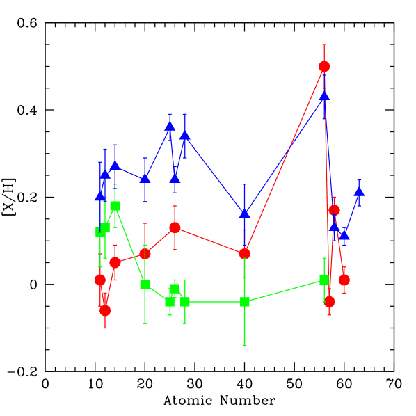
Figure 5.— Abundance patterns of the three studied clusters. The Hyades is shown in red circles, Collinder 261 is in green squares, and the HR1614 moving group is in blue triangles. The three cluster have their own abundance patterns.

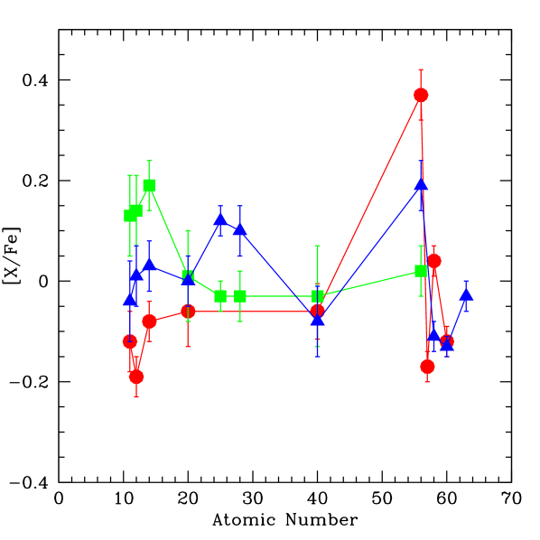
Figure 6.— Abundances relative to Fe for the three studied clusters. The symbols are same as those in Figure 5. The three clusters still show unique signatures, demonstrating that abundance patterns are not always locked to Fe. Note Fe is not plotted.

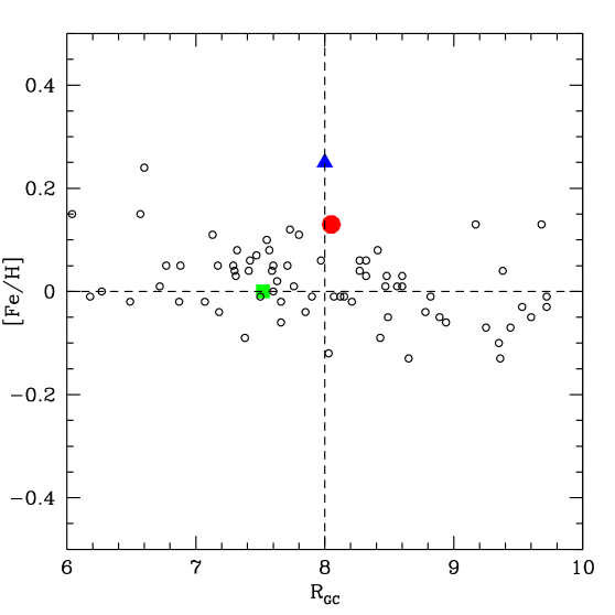
Figure 7.— Metallicity vs. Galactocentric radius for cepheids and the studied clusters. The open circles are the cepheid abundances from Andrievsky et al. (2002). The cluster symbols are same as those in Figure 5. The dashed lines mark the Sun.

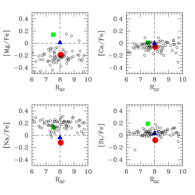
Figure 8.— [X/Fe] vs. Galactocentric radius for cepheids and the studied clusters.The open circles are the cepheid abundances from Andrievsky et al. (2002). The cluster symbols are same as those in Figure 5. The dashed lines mark the Sun.

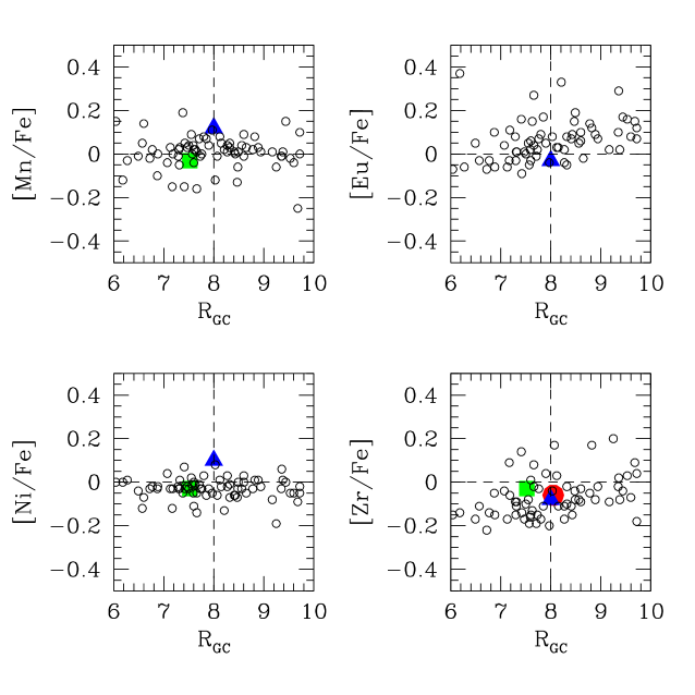
Figure 9.— [X/Fe] vs. Galactocentric radius for cepheids and the studied clusters.The open circles are the cepheid abundances from Andrievsky et al. (2002). The cluster symbols are same as those in Figure 5. The dashed lines mark the Sun.

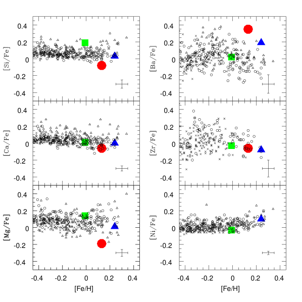
Figure 10.— Cluster abundances compared to the field surveys. The open circles represent Reddy et al. (2003) values, crosses represent Edvardsson et al. (1993) values, and triangles represent Allende Prieto et al. (2004) values. The cluster symbols are same as those in Figure 5. The error bars are from Reddy et al. (2003).

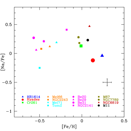
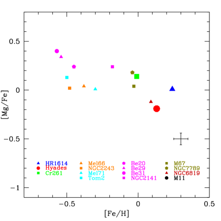
Figure 11.— Na and Mg abundances for open clusters.

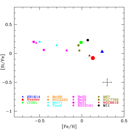
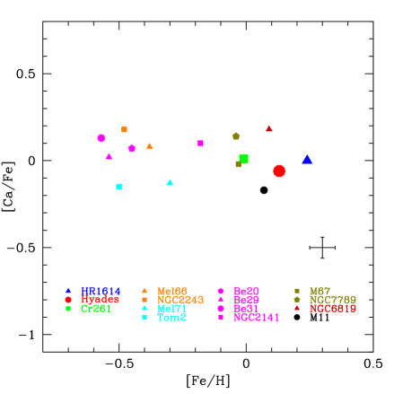
Figure 12.— Si and Ca abundances for open clusters.

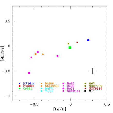
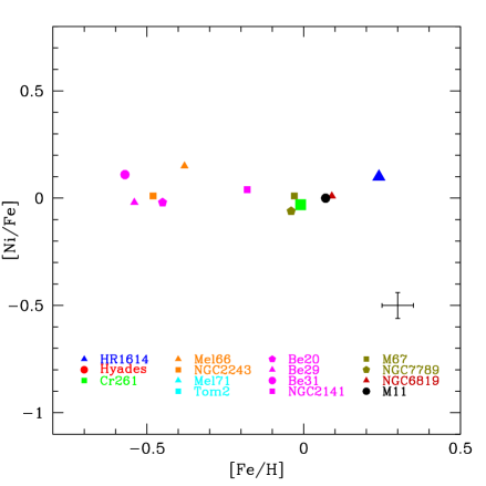
Figure 13.— Mn and Ni abundances for open clusters.

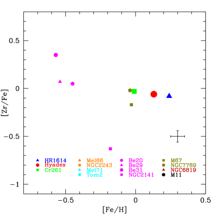
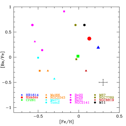
Figure 14.— The s-process element abundances for open clusters.

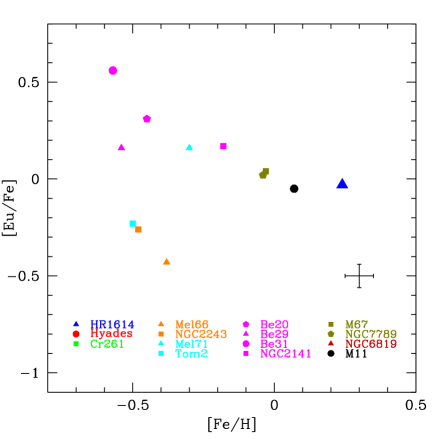
Figure 15.— Eu (r-process) abundances for open clusters.

Table 1Collinder 261 Stellar Sample

ID (G96)	ID (PJM)	RA	DEC	V	V-I
2268	2001	12 37 38.681	-68 20 25.87	13.99	1.37
2277	1801	12 37 45.396	-68 24 1.02	13.61	1.36
2285	1526	12 37 54.105	-68 21 48.48	14.27	1.42
2288	1481	12 37 55.375	-68 22 35.76	13.95	1.51
2289	1485	12 37 55.557	-68 20 14.36	13.74	1.60
2291	1472	12 37 55.504	-68 24 49.52	13.51	1.32
2306	1080	12 38 7.420	-68 22 30.82	13.95	1.48
2307	1045	12 38 8.499	-68 21 15.01	13.58	1.53
2311	906	12 38 12.512	-68 20 31.45	14.21	1.44
3027	27	12 38 40.824	-68 23 39.13	13.89	1.66
3029	29	12 38 40.772	-68 23 55.46	14.31	1.49
3709	1871	12 37 43.608	-68 19 55.06	12.43	1.84

Table 2Line list

Wavelength(Å)	Species	LEP(eV)	log $gf$		Wavelength(Å)	Species	LEP(eV)	log $gf$		Wavelength(Å)	Species	LEP(eV)	log $gf$
5688.19	Na i	2.11	$-$0.420		4489.74	Fe i	0.12	$-$3.966		6082.72	Fe i	2.22	$-$3.650
6154.23	Na i	2.10	$-$1.530		4494.57	Fe i	2.20	$-$1.136		6093.64	Fe i	4.61	$-$1.510
6160.75	Na i	2.10	$-$1.230		4523.40	Fe i	3.65	$-$1.990		6094.37	Fe i	4.65	$-$1.650
4571.09	Mg i	0.00	$-$5.393		4531.15	Fe i	1.48	$-$2.155		6096.66	Fe i	3.98	$-$1.880
4702.99	Mg i	4.33	$-$0.380		4531.58	Fe i	3.93	$-$2.059		6105.13	Fe i	4.55	$-$1.990
5711.09	Mg i	4.35	$-$1.833		4547.85	Fe i	3.54	$-$1.012		6120.24	Fe i	0.91	$-$5.970
5665.56	Si i	4.92	$-$1.940		4556.93	Fe i	3.25	$-$2.710		6151.62	Fe i	2.17	$-$3.299
5684.49	Si i	4.95	$-$1.550		4561.43	Fe i	2.76	$-$3.080		6157.73	Fe i	4.08	$-$1.320
5690.43	Si i	4.93	$-$1.770		4593.52	Fe i	3.94	$-$2.060		6159.38	Fe i	4.61	$-$1.970
5948.54	Si i	5.08	$-$1.230		4602.01	Fe i	1.61	$-$3.154		6173.34	Fe i	2.22	$-$2.880
6142.48	Si i	5.62	$-$1.540		5379.57	Fe i	3.68	$-$1.730		6180.20	Fe i	2.73	$-$2.637
6145.01	Si i	5.62	$-$1.362		5417.03	Fe i	4.41	$-$1.550		6200.31	Fe i	2.61	$-$2.437
6155.13	Si i	5.62	$-$0.786		5466.99	Fe i	3.57	$-$2.440		4491.41	Fe ii	2.86	$-$2.684
4455.88	Ca i	1.89	$-$0.526		5618.63	Fe i	4.21	$-$1.292		4508.28	Fe ii	2.86	$-$2.312
4578.55	Ca i	2.25	$-$0.558		5633.95	Fe i	4.99	$-$0.270		4541.52	Fe ii	2.84	$-$2.990
5867.57	Ca i	2.93	$-$1.570		5662.52	Fe i	4.16	$-$0.520		4576.33	Fe ii	2.84	$-$2.822
6169.04	Ca i	2.52	$-$0.797		5701.55	Fe i	2.56	$-$2.216		4582.83	Fe ii	2.84	$-$3.094
6169.56	Ca i	2.53	$-$0.478		5705.47	Fe i	4.30	$-$1.420		4620.52	Fe ii	2.83	$-$3.079
6013.53	Mn i	3.07	$-$0.251		5741.85	Fe i	4.25	$-$1.689		4656.98	Fe ii	2.89	$-$3.552
6016.67	Mn i	3.08	$-$0.100		5775.08	Fe i	4.22	$-$1.310		4670.17	Fe ii	2.58	$-$3.904
6021.80	Mn i	3.08	0.034		5778.45	Fe i	2.59	$-$3.480		5414.08	Fe ii	3.22	$-$3.680
4216.19	Fe i	0.00	$-$3.356		5811.92	Fe i	4.14	$-$2.430		5991.38	Fe ii	3.15	$-$3.557
4222.22	Fe i	2.45	$-$0.967		5837.70	Fe i	4.29	$-$2.340		6084.11	Fe ii	3.20	$-$3.808
4232.72	Fe i	0.11	$-$4.928		5853.16	Fe i	1.49	$-$5.280		6149.26	Fe ii	3.89	$-$2.724
4233.61	Fe i	2.48	$-$0.604		5855.09	Fe i	4.60	$-$1.547		5846.99	Ni i	1.68	$-$3.210
4237.09	Fe i	0.95	$-$4.379		5856.10	Fe i	4.29	$-$1.640		6086.28	Ni i	4.26	$-$0.515
4347.24	Fe i	0.00	$-$5.503		5858.79	Fe i	4.22	$-$2.260		6175.37	Ni i	4.09	$-$0.535
4375.93	Fe i	0.00	$-$3.031		5927.80	Fe i	4.65	$-$1.090		6177.24	Ni i	1.83	$-$3.510
4389.24	Fe i	0.05	$-$4.583		5956.69	Fe i	0.86	$-$4.608		6127.44	Zr i	0.15	$-$1.060
4439.88	Fe i	2.28	$-$3.002		6015.24	Fe i	2.22	$-$4.760		6134.55	Zr i	0.00	$-$1.280
4442.34	Fe i	2.19	$-$1.255		6024.06	Fe i	4.54	0.610		6143.20	Zr i	0.07	$-$1.100
4445.48	Fe i	0.08	$-$5.441		6034.03	Fe i	4.31	$-$2.470		5853.69	Ba ii	0.60	$-$1.010
4447.72	Fe i	2.22	$-$1.342		6042.22	Fe i	4.65	$-$0.890		6141.73	Ba ii	0.70	$-$0.070
4427.31	Fe i	0.05	$-$3.044		6054.08	Fe i	4.37	$-$2.310		$\cdots$	$\cdots$	$\cdots$	$\cdots$
4461.65	Fe i	0.08	$-$5.441		6056.00	Fe i	4.73	$-$0.650		$\cdots$	$\cdots$	$\cdots$	$\cdots$

Table 3Stellar Parameters

ID	Teff	Log $g$	$\xi$	Teff (C05)	Log $g$ (C05)	$\xi$(C05)	Teff (F03)	Log $g$ (F03)	$\xi$(F03)
2268	4550	2.0	1.52	4580	1.83	1.26	$\cdots$	$\cdots$	$\cdots$
2277	4600	2.0	1.4	$\cdots$	$\cdots$	$\cdots$	$\cdots$	$\cdots$	$\cdots$
2285	4600	2.0	0.9	$\cdots$	$\cdots$	$\cdots$	$\cdots$	$\cdots$	$\cdots$
2288	4400	2.1	1.2	$\cdots$	$\cdots$	$\cdots$	$\cdots$	$\cdots$	$\cdots$
2289	4300	1.8	1.4	4340	1.76	1.27	$\cdots$	$\cdots$	$\cdots$
2291	4650	2.3	1.8	$\cdots$	$\cdots$	$\cdots$	$\cdots$	$\cdots$	$\cdots$
2306	4500	2.1	1.5	4500	2.09	1.23	4900	2.2	1.2
2307	4450	1.8	1.1	4470	2.07	1.23	4400	1.5	1.2
2311	4600	2.0	0.9	$\cdots$	$\cdots$	$\cdots$	$\cdots$	$\cdots$	$\cdots$
3027	4500	2.0	1.2	$\cdots$	$\cdots$	$\cdots$	$\cdots$	$\cdots$	$\cdots$
3029	4500	1.9	1.4	$\cdots$	$\cdots$	$\cdots$	$\cdots$	$\cdots$	$\cdots$
3709	3950	0.5	1.4	3980	0.43	1.44	4000	0.7	1.5

Table 4Absolute Abundances (log $\epsilon$)

ID	Na	Mg	Si	Ca	Mn	Fe	Ni	Zr	Ba (with HFS)	Ba (without HFS)
2268	6.61	7.65	7.79	6.44	5.40	7.52	6.17	2.63	2.15	2.36
2277	6.49	7.78	7.78	6.28	5.39	7.51	6.15	2.66	2.17	2.27
2285	6.44	7.71	7.68	6.34	5.32	7.52	6.24	2.66	2.14	2.34
2288	6.36	7.80	7.68	6.39	5.35	7.49	6.26	2.41	2.13	2.34
2289	6.42	7.69	7.76	6.37	5.39	7.50	6.27	2.57	2.17	2.29
2291	6.45	7.67	7.66	6.29	5.39	7.51	6.19	2.70	2.13	2.25
2306	6.32	7.71	7.75	6.37	5.34	7.54	6.16	2.45	2.14	2.30
2307	6.48	7.75	7.80	6.38	5.29	7.51	6.22	2.31	2.15	2.31
2311	6.65	7.89	7.85	6.61	5.44	7.56	6.33	2.73	2.37	2.47
3027	6.46	7.75	7.78	6.43	5.34	7.53	6.21	2.64	2.13	2.23
3029	6.44	7.69	7.70	6.33	5.35	7.49	6.18	2.54	2.14	2.38
3709	6.44	7.61	7.66	6.32	5.35	7.51	6.15	2.57	2.15	2.30

Table 5Abundance dependencies on model atmospheres (Kurucz - MARCS)

Star	$\delta$[Na/H]	$\delta$[Mg/H]	$\delta$[Si/H]	$\delta$[Ca/H]	$\delta$[Mn/H]	$\delta$[Fe/H]	$\delta$[Ni/H]	$\delta$[Zr/H]	$\delta$[Ba/H]
2285 (Teff = 4600K)	$-$0.01	0.00	0.01	$-$0.01	$-$ 0.01	0.01	0.00	$-$ 0.02	0.03
2288 (Teff = 4400K)	0.04	$-$ 0.01	$-$ 0.07	0.05	0.00	$-$ 0.03	$-$ 0.11	0.00	$-$ 0.06
3709 (Teff = 3950K)	0.15	0.01	0.02	0.17	0.05	0.01	0.02	0.35	0.06

Table 6Abundance dependencies on model atmospheres (Kurucz - MARCS) with adjusted microturbulence

Star	$\delta$[Na/H]	$\delta$[Mg/H]	$\delta$[Si/H]	$\delta$[Ca/H]	$\delta$[Mn/H]	$\delta$[Fe/H]	$\delta$[Ni/H]	$\delta$[Zr/H]	$\delta$[Ba/H]
2285 (Teff = 4600K)	0.01	0.00	$-$ 0.01	0.01	$-$ 0.02	$-$ 0.02	$-$ 0.02	$-$ 0.02	0.00
2288 (Teff = 4400K)	0.04	$-$ 0.01	$-$ 0.04	0.05	0.00	$-$ 0.03	$-$ 0.04	0.00	$-$ 0.06
3709 (Teff = 3950K)	0.03	0.01	0.02	0.01	0.00	0.01	0.02	0.07	0.06

Table 7Abundance Sensitivities for star 2268

	$\delta$[Fe/H]	$\delta$[Na/H]	$\delta$[Mg/H]	$\delta$[Si/H]	$\delta$[Ca/H]	$\delta$[Mn/H]	$\delta$[Ni/H]	$\delta$[Zr/H]	$\delta$[Ba/H]
$\Delta$ T${}_{\rm eff}=\pm$50	$\pm$0.01	$\pm$0.04	$\pm$0.02	$\mp$0.03	$\pm$0.04	$\pm$0.00	$\pm$0.01	$\pm$0.10	0.00
$\Delta$ log $g$ = $\pm$0.1	$\pm$0.02	$\mp$0.02	0.00	$\pm$0.02	$\mp$0.00	$\mp$0.01	$\pm$0.03	$\pm$0.01	$\pm$0.05
$\Delta\xi=\pm$0.2	$\mp$0.02	$\mp$0.04	$\mp$0.04	$\mp$0.03	$\mp$0.05	$\mp$0.02	$\mp$0.04	$\mp$0.04	$\mp$0.05
$\Delta$ EW	$\pm$0.01	$\pm$0.05	$\pm$0.04	$\pm$0.03	$\pm$0.02	$\pm$0.02	$\pm$0.01	$\pm$0.07	$\pm$0.02
Total	$\pm$0.03	$\pm$0.08	$\pm$0.06	$\pm$0.05	$\pm$0.06	$\pm$0.04	$\pm$0.05	$\pm$0.13	$\pm$0.08

Table 8Radial Velocities

Star ID	this study	Friel et al. (2002)
2268	-24.5	-35
2277	-24.2	-35
2285	-26.9	-28
2288	-27.3	-27
2289	-27.2	-35
2291	-27.8	-31
2306	-28.1	-31
2307	-26.3	-30
2311	-18.1	-30
3027	-24.5	-31
3029	-24.2	-16
3709	-28.2	-37

Table 9Abundance scatter

Element	$\sigma_{obs}$	$\sigma_{int}$ (upper)
Fe	0.02	0.02
Na	0.07	0.04
Mg	0.05	0.04
Si	0.06	0.05
Ca	0.05	0.04
Mn	0.03	0.02
Ni	0.04	0.03
Zr	0.12	0.05
Ba	0.03	0.02

Table 10Cluster Abundance Summary

Atomic No	[X/H]	Hyades	$\sigma$	Collinder 261	$\sigma$	HR 1614	$\sigma$	Adopted Solar
26	Fe	0.13	0.05	-0.01	0.02	0.24	0.03	7.52
11	Na	0.01	0.06	0.12	0.08	0.20	0.08	6.33
12	Mg	-0.06	0.04	0.13	0.07	0.25	0.06	7.58
14	Si	0.05	0.04	0.18	0.05	0.27	0.05	7.55
20	Ca	0.07	0.07	0.00	0.09	0.24	0.05	6.36
25	Mn	$\cdots$	$\cdots$	-0.04	0.03	0.36	0.03	5.39
28	Ni	$\cdots$	$\cdots$	-0.04	0.05	0.34	0.05	6.25
40	Zr	0.07	0.06	-0.04	0.10	0.16	0.07	2.60
56	Ba	0.50	0.05	0.01	0.03	0.43	0.05	2.13
58	Ce	0.17	0.03	$\cdots$	$\cdots$	0.13	0.03	1.58
60	Nd	0.01	0.03	$\cdots$	$\cdots$	0.11	0.02	1.45
63	Eu	$\cdots$	$\cdots$	$\cdots$	$\cdots$	0.21	0.03	0.52

References

- Allende Prieto et al. (2002) Allende Prieto, C., Asplund, M., López, R. J. G., & Lambert, D. L. 2002, ApJ, 567, 544
- Allende Prieto et al. (2004) Allende Prieto, C., Barklem, P. S., Lambert, D. L., & Cunha, K. 2004, A&A, 420, 183
- Andrievsky et al. (2002) Andrievsky, S. M., Kovtyukh, V. V., Luck, R. E., Lépine, J. R. D., Bersier, D., Maciel, W. J., Barbuy, B., Klochkova, V. G., Panchuk, V. E., & Karpischek, R. U. 2002, A&A, 381, 32
- Asplund (2005) Asplund, M. 2005, ARA&A, 43, 481
- Asplund et al. (1997) Asplund, M., Gustafsson, B., Kiselman, D., & Eriksson, K. 1997, A&A, 318, 521
- Bensby et al. (2003) Bensby, T., Feltzing, S., & Lundström, I. 2003, A&A, 410, 527
- Biemont et al. (1991) Biemont, E., Baudoux, M., Kurucz, R. L., Ansbacher, W., & Pinnington, E. H. 1991, A&A, 249, 539
- Bland-Hawthorn & Freeman (2004) Bland-Hawthorn, J., & Freeman, K. C. 2004, Publications of the Astronomical Society of Australia, 21, 110
- Bragaglia et al. (2001) Bragaglia, A., Carretta, E., Gratton, R. G., Tosi, M., Bonanno, G., Bruno, P., Calì, A., Claudi, R., Cosentino, R., Desidera, S., Farisato, G., Rebeschini, M., & Scuderi, S. 2001, AJ, 121, 327
- Brown et al. (1996) Brown, J. A., Wallerstein, G., Geisler, D., & Oke, J. B. 1996, AJ, 112, 1551
- Carraro et al. (1998) Carraro, G., Ng, Y. K., & Portinari, L. 1998, MNRAS, 296, 1045
- Carretta et al. (2005) Carretta, E., Bragaglia, A., Gratton, R. G., & Tosi, M. 2005, A&A, 441, 131
- Castelli et al. (1997) Castelli, F., Gratton, R. G., & Kurucz, R. L. 1997, A&A, 318, 841
- Conti et al. (1965) Conti, P. S., Wallerstein, G., & Wing, R. F. 1965, ApJ, 142, 999
- De Silva et al. (in press) De Silva, G. M., Freeman, K. C., Bland-Hawthorn, J., Asplund, M., & Bessell, M. S., AJ, in press (astro-ph/0610041)
- De Silva et al. (2006) De Silva, G. M., Sneden, C., Paulson, D. B., Asplund, M., Bland-Hawthorn, J., Bessell, M. S., & Freeman, K. C. 2006, AJ, 131, 455
- Den Hartog et al. (2003) Den Hartog, E. A., Lawler, J. E., Sneden, C., & Cowan, J. J. 2003, ApJS, 148, 543
- Edvardsson et al. (1993) Edvardsson, B., Andersen, J., Gustafsson, B., Lambert, D. L., Nissen, P. E., & Tomkin, J. 1993, A&A, 275, 101
- Ford et al. (2005) Ford, A., Jeffries, R. D., & Smalley, B. 2005, MNRAS, 364, 272
- Freeman & Bland-Hawthorn (2002) Freeman, K., & Bland-Hawthorn, J. 2002, ARA&A, 40, 487
- Friel (1995) Friel, E. D. 1995, ARA&A, 33, 381
- Friel et al. (2003) Friel, E. D., Jacobson, H. R., Barrett, E., Fullton, L., Balachandran, S. C., & Pilachowski, C. A. 2003, AJ, 126, 2372
- Friel et al. (2002) Friel, E. D., Janes, K. A., Tavarez, M., Scott, J., Katsanis, R., Lotz, J., Hong, L., & Miller, N. 2002, AJ, 124, 2693
- Gonzalez & Wallerstein (2000) Gonzalez, G., & Wallerstein, G. 2000, PASP, 112, 1081
- Gozzoli et al. (1996) Gozzoli, E., Tosi, M., Marconi, G., & Bragaglia, A. 1996, MNRAS, 283, 66
- Gratton et al. (2004) Gratton, R., Sneden, C., & Carretta, E. 2004, ARA&A, 42, 385
- Gratton & Contarini (1994) Gratton, R. G., & Contarini, G. 1994, A&A, 283, 911
- Grevesse & Sauval (1998) Grevesse, N., & Sauval, A. J. 1998, Space Science Reviews, 85, 161
- Janes & Phelps (1994) Janes, K. A., & Phelps, R. L. 1994, AJ, 108, 1773
- Kurtz & Mink (1998) Kurtz, M. J., & Mink, D. J. 1998, PASP, 110, 934
- Kurtz et al. (1992) Kurtz, M. J., Mink, D. J., Wyatt, W. F., Fabricant, D. G., Torres, G., Kriss, G. A., & Tonry, J. L. 1992, in ASP Conf. Ser. 25: Astronomical Data Analysis Software and Systems I, 432–+
- Lawler et al. (2001) Lawler, J. E., Wickliffe, M. E., den Hartog, E. A., & Sneden, C. 2001, ApJ, 563, 1075
- McWilliam (1998) McWilliam, A. 1998, ApJ, 115, 1640
- McWilliam et al. (2003) McWilliam, A., Rich, R. M., & Smecker-Hane, T. A. 2003, ApJ, 592, L21
- Pagel & Tautvaisiene (1997) Pagel, B. E. J., & Tautvaisiene, G. 1997, MNRAS, 288, 108
- Paulson et al. (2003) Paulson, D. B., Sneden, C., & Cochran, W. D. 2003, AJ, 125, 3185
- Phelps et al. (1994) Phelps, R. L., Janes, K. A., & Montgomery, K. A. 1994, AJ, 107, 1079
- Prochaska & McWilliam (2000) Prochaska, J. X., & McWilliam, A. 2000, ApJ, 537, L57
- Prochaska et al. (2000) Prochaska, J. X., Naumov, S. O., Carney, B. W., McWilliam, A., & Wolfe, A. M. 2000, AJ, 120, 2513
- Reddy et al. (2003) Reddy, B. E., Tomkin, J., Lambert, D. L., & Allende Prieto, C. 2003, MNRAS, 340, 304
- Schuler et al. (2003) Schuler, S. C., King, J. R., Fischer, D. A., Soderblom, D. R., & Jones, B. F. 2003, AJ, 125, 2085
- Shetrone et al. (2003) Shetrone, M., Venn, K. A., Tolstoy, E., Primas, F., Hill, V., & Kaufer, A. 2003, AJ, 125, 684
- Sneden et al. (1992) Sneden, C., Kraft, R. P., Prosser, C. F., & Langer, G. E. 1992, AJ, 104, 2121
- Sneden (1973) Sneden, C. A. 1973, Ph.D. Thesis
- Tautvaišienė et al. (2005) Tautvaišienė, G., Edvardsson, B., Puzeras, E., & Ilyin, I. 2005, A&A, 431, 933
- Tautvaišiene et al. (2000) Tautvaišiene, G., Edvardsson, B., Tuominen, I., & Ilyin, I. 2000, A&A, 360, 499
- Yong et al. (2005) Yong, D., Carney, B. W., & de Almeida, M. L. T. 2005, AJ, 130, 597
- Zwitter et al. (2004) Zwitter, T., Castelli, F., & Munari, U. 2004, A&A, 417, 1055