Cosmological Simulations using Grid Middleware

1 Introduction

One way to access the aggregated power of a collection of heterogeneous machines is to use a grid middleware, such as Diet [1], GridSolve [7] or Ninf [4]. It addresses the problem of monitoring the resources, of handling the submissions of jobs and as an example the inherent transfer of input and output data, in place of the user.

In this paper we present how to run cosmological simulations using the Ramses application along with the Diet middleware. We will describe how to write the corresponding Diet client and server. The remainder of the paper is organized as follows: Section 2 presents the Diet middleware. Section 3 describes the Ramses cosmological software and simulations, and how to interface it with Diet. We show how to write a client and a server in Section 4. Finally, Section 5 presents the experiments realized on Grid’5000, the French Research Grid, and we conclude in Section 6.

2 DIET overview

2.1 DIET architecture

Diet [1] is built upon the client/agent/server paradigm. A Client is an application that uses Diet to solve problems. Different kinds of clients should be able to connect to Diet: from a web page, a PSE such as Matlab or Scilab, or from a program written in C or Fortran. Computations are done by servers running a Server Daemons (SeD). A SeD encapsulates a computational server. For instance it can be located on the entry point of a parallel computer. The information stored by a SeD is a list of the data available on its server, all information concerning its load (for example available memory and processor) and the list of problems that it can solve. The latter are declared to its parent agent. The hierarchy of scheduling agents is made of a Master Agent (MA) and Local Agents (LA) (see Figure 1).

When a Master Agent receives a computation request from a client, agents collect computation abilities from servers (through the hierarchy) and chooses the best one according to some scheduling heuristics. The MA sends back a reference to the chosen server. A client can be connected to a MA by a specific name server or by a web page which stores the various MA locations (and the available problems). The information stored on an agent is the list of requests, the number of servers that can solve a given problem and information about the data distributed in its subtree. For performance reasons, the hierachy of agents sould be deployed depending on the underlying network topology.

Finally, on the opposite of GridSolve and Ninf which rely on a classic socket communication layer (nevertheless several problems to this approach have been pointed out such as the lack of portability or the limitation of opened sockets), Diet uses Corba. Indeed, distributed object environments, such as Java, DCOM or Corba have proven to be a good base for building applications that manage access to distributed services. They provide transparent communications in heterogeneous networks, but they also offer a framework for the large scale deployment of distributed applications. Moreover, Corba systems provide a remote method invocation facility with a high level of transparency which does not affect performance [3].

2.2 How to add a new grid application within Diet?

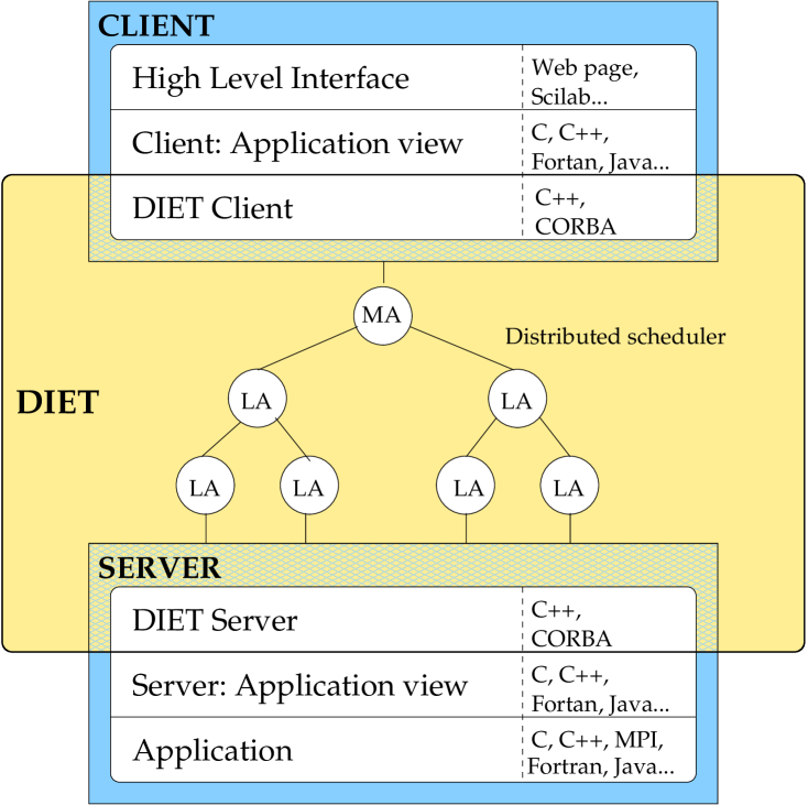
Figure 1: Different interaction layers between Diet core and application view

The main idea is to provide some integrated level for a grid application. Figure 1 shows these different kinds of level.

The application server must be written to give Diet the ability to use the application. A simple API is available to easily provide a connection between the Diet server and the application. The main goals of the Diet server are to answer to monitoring queries from its responsible Local Agent and launch the resolution of a service, upon an application client request.

The application client is the link between high-level interface and the Diet client, and a simple API is provided to easily write one. The main goals of the Diet client are to submit requests to a scheduler (called Master Agent) and to receive the identity of the chosen server, and final step, to send the data to the server for the computing phase.

3 Ramses overview

Ramses is a typical computational intensive application used by astrophysicists to study the formation of galaxies. Ramses is used, among other things, to simulate the evolution of a collisionless, self-gravitating fluid called “dark matter” through cosmic time (see Figure 2). Individual trajectories of macro-particles are integrated using a state-of-the-art “N body solver”, coupled to a finite volume Euler solver, based on the Adaptive Mesh Refinement technics. The computational space is decomposed among the available processors using a mesh partitionning strategy based on the Peano–Hilbert cell ordering ([5, 6]).

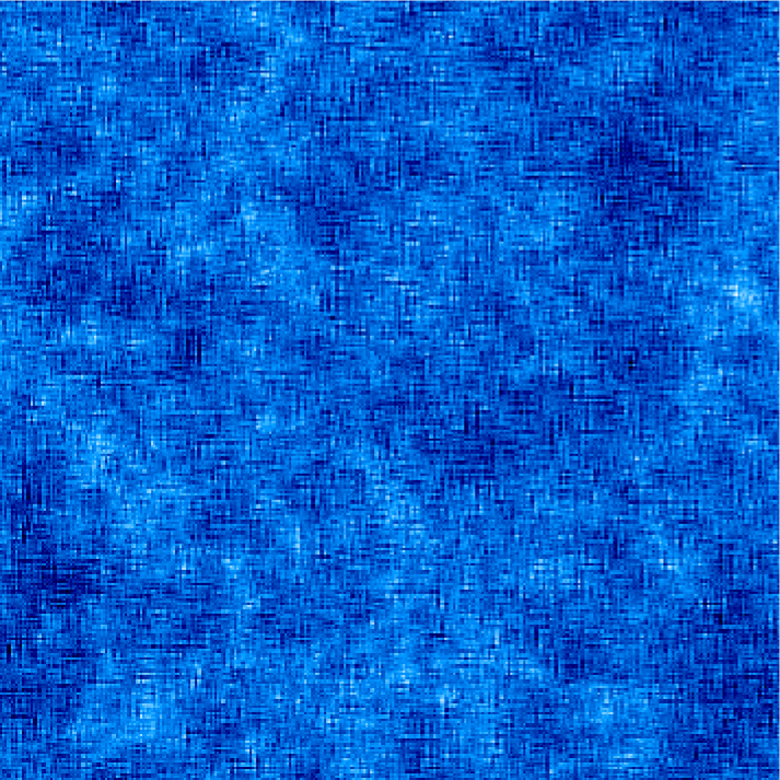
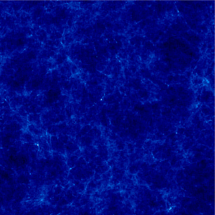
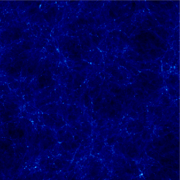
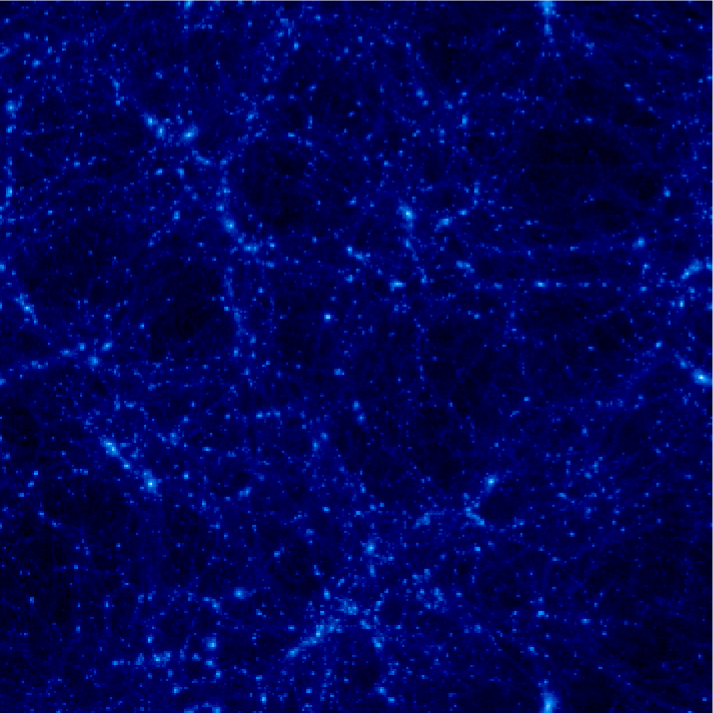
Figure 2: Time sequence (from left to right) of the projected density field in a cosmological simulation (large scale periodic box).

Cosmological simulations are usually divided into two main categories. Large scale periodic boxes (see Figure 2) requiring massively parallel computers are performed on very long elapsed time (usually several months). The second category stands for much faster small scale “zoom simulations”. One of the particularity of the HORIZON project is that it allows the re-simulation of some areas of interest for astronomers.

For example in Figure 3, a supercluster of galaxies has been chosen to be re-simulated at a higher resolution (highest number of particules) taking the initial information and the boundary conditions from the larger box (of lower resolution). This is the latter category we are interested in. Performing a zoom simulation requires two steps: the first step consists of using Ramses on a low resolution set of initial conditions i.e., with a small number of particles) to obtain at the end of the simulation a catalog of “dark matter halos”, seen in Figure 2 as high-density peaks, containing each halo position, mass and velocity. A small region is selected around each halo of the catalog, for which we can start the second step of the “zoom” method. This idea is to resimulate this specific halo at a much better resolution. For that, we add in the Lagrangian volume of the chosen halo a lot more particles, in order to obtain more accurate results. Similar “zoom simulations” are performed in parallel for each entry of the halo catalog and represent the main resource consuming part of the project.

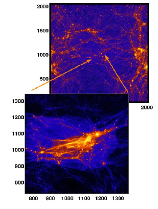
Figure 3: Re-simulation on a supercluster of galaxies to increase the resolution

Ramses simulations are started from specific initial conditions, containing the initial particle masses, positions and velocities. These initial conditions are read from Fortran binary files, generated using a modified version of the Grafic code. This application generates Gaussian random fields at different resolution levels, consistent with current observational data obtained by the WMAP satellite observing the cosmic microwave background radiation. Two types of initial conditions can be generated with Grafic:

• single level: this is the “standard” way of generating initial conditions. The resulting files are used to perform the first, low-resolution simulation, from which the halo catalog is extracted.

• multiple levels: this initial conditions are used for the “zoom simulation”. The resulting files consist of multiple, nested boxes of smaller and smaller dimensions, as for Russian dolls. The smallest box is centered around the halo region, for which we have locally a very high accuracy thanks to a much larger number of particles.

The result of the simulation is a set of ”snaphots”. Given a list of time steps (or expansion factor), Ramses outputs the current state of the universe (i.e., the different parameters of each particules) in Fortran binary files. These files need post-processing with Galics softwares: HaloMaker, TreeMaker and GalaxyMaker. These three softwares are meant to be used sequentially, each of them producing different kinds of information:

• HaloMaker: detects dark matter halos present in Ramses output files, and creates a catalog of halos

• TreeMaker: given the catalog of halos, TreeMaker builds a merger tree: it follows the position, the mass, the velocity of the different particules present in the halos through cosmic time

• GalaxyMaker: applies a semi-analytical model to the results of TreeMaker to form galaxies, and creates a catalog of galaxies

4 Interfacing Ramses within Diet

4.1 Architecture of underlying deployment

The current version of Ramses requires a NFS working directory in order to write the output files, hence restricting the possible types of solving architectures. Each Diet server will be in charge of a set of machines (typically 32 machines to run a $256^{3}$ particules simulation) belonging to the same cluster. For each simulation the generation of the initial conditions files, the processing and the post-processing are done on the same cluster: the server in charge of a simulation manages the whole process.

4.2 Server design

The Diet server is a library. So the Ramses server requires to define the main() function, which contains the problem profile definition and registration, and the solving function, whose parameter only consists of the profile and named after the service name, solve_serviceName.

The Ramses solving function contains the calls to the different programs used for the simulation, and which will manage the MPI environment required by Ramses. It is recorded during the profile registration.

The SeD is launched with a call to diet_SeD() in the main() function, which will never return (except if some errors occur). The SeD forks the solving function when requested.

4.2.1 Defining services

To match client requests with server services, clients and servers must use the same problem description. A unified way to describe problems is to use a name and define its arguments. The Ramses service is described by a profile description structure called diet_profile_desc_t. Among its fields, it contains the name of the service, an array which does not contain data, but their characteristics, and three integers last_in, last_inout and last_out. The structure is defined in DIET_server.h.

The array is of size $last\_out+1$. Arguments can be:

IN: Data are sent to the server. The memory is allocated by the user.

INOUT: Data, allocated by the user, are sent to the server and brought back into the same memory zone after the computation has completed, without any copy. Thus freeing this memory while the computation is performed on the server would result in a segmentation fault when data are brought back onto the client.

OUT: Data are created on the server and brought back into a newly allocated zone on the client. This allocation is performed by Diet. After the call has returned, the user can find its result in the zone pointed at by the value field. Of course, Diet cannot guess how long the user needs these data for, so it lets him/her free the memory with diet_free_data().

The fields last_in, last_inout and last_out of the structure respectively point at the indexes in the array of the last IN, last INOUT and last OUT arguments.

Functions to create and destroy such profiles are defined with the prototypes below. Note that if a server can solve multiple services, each profile should be allocated.

⬇

diet_profile_desc_t *diet_profile_desc_alloc( const char* path, int last_in, int last_inout, int last_out );

diet_profile_desc_t *diet_profile_desc_alloc( int last_in, int last_inout, int last_out );

int diet_profile_desc_free(diet_profile_desc_t *desc);

The cosmological simulation is divided in two services: ramsesZoom1 and ramsesZoom2, they represent the two parts of the simulation. The first one is used to determine interesting parts of the universe, while the second is used to study these parts in details. The ramsesZoom2 service uses nine data. The seven firsts are IN data, and contain the simulation parameters:

• a file containing parameters for Ramses

• resolution of the simulation (number of particules)

• size of the initial conditions (in $Mpc.h^{-1}$)

• center’s coordinates of the initial conditions (3 coordinates: $c_{x}$, $c_{y}$ and $c_{z}$)

• number of zoom levels (number of nested boxes)

The last two are an integer for error controls, and a file containing the results obtained from the simulation post-processed with Galics. This conducts to the following inclusion in the server code (note: the same allocation must be performed on the client side, with the diet_profile_t structure):

⬇

/* arg.profile is a diet_profile_desc_t * */

arg.profile = diet_profile_desc_alloc("ramsesZoom2", 6, 6, 8);

Every argument of the profile must then be set with diet_generic_desc_set() defined in DIET_server.h, like:

⬇

diet_generic_desc_set(diet_parameter(pb,0), DIET_FILE, DIET_CHAR);

diet_generic_desc_set(diet_parameter(pb,1), DIET_SCALAR, DIET_INT);

4.2.2 Registering services

Every defined service has to be added in the service table before the SeD is launched. The complete service table API is defined in DIET_server.h:

⬇

typedef int (* diet_solve_t)(diet_profile_t *);

int diet_service_table_init(int max_size);

int diet_service_table_add(diet_profile_desc_t *profile, NULL, diet_solve_t solve_func);

void diet_print_service_table();

The first parameter, profile, is a pointer on the profile previously described (section 4.2.1). The second parameter concerns the convertor functionality, but this is out of scope of this paper and never used for this application. The parameter solve_func is the type of the solve_serviceName() function: a function pointer used by Diet to launch the computation. Here, the prototype is then:

⬇

int solve_ramsesZoom2(diet_profile_t* pb)

{

/* Data downloading */

/* Computation */

/* Data uploading */

}

4.2.3 Data management

The first part of the solve function (called solve_ramsesZoom2()) is to receive data. The API provides useful functions to help coding the solve function, e.g., get IN arguments, set OUT ones, with diet_*_get() functions defined in DIET_data.h. Do not forget that the necessary memory space for OUT arguments is allocated by Diet. So the user should call the diet_*_get() functions to retrieve the pointer to the zone his/her program should write to. To set INOUT and OUT arguments, one should use the diet_*_desc_set() defined in DIET_server.h. These should be called within “solve” functions only.

⬇

diet_file_get(diet_parameter(pb,0), NULL, &arg_size, &nmlPath);

diet_scalar_get(diet_parameter(pb,1), &resol, NULL);

diet_scalar_get(diet_parameter(pb,2), &size, NULL);

diet_scalar_get(diet_parameter(pb,3), &cx, NULL);

diet_scalar_get(diet_parameter(pb,4), &cy, NULL);

diet_scalar_get(diet_parameter(pb,5), &cz, NULL);

diet_scalar_get(diet_parameter(pb,6), &nbBox, NULL);

The results of the simulation are packed into a tarball file if it succeeded. Thus we need to return this file and an error code to inform the client whether the file really contains results or not. In the following code, the diet_file_set() function associate the Diet parameter with the current file. Indeed, the data should be available for Diet, when it sends the resulting file to the client.

⬇

char* tgzfile = NULL;

tgzfile = (char*)malloc(tarfile.length()+1);

strcpy(tgzfile, tarfile.c_str());

diet_file_set(diet_parameter(pb,7), DIET_VOLATILE, tgzfile);

4.3 Client

In the Diet architecture, a client is an application which uses Diet to request a service. The goal of the client is to connect to a Master Agent in order to dispose of a SeD which will be able to solve the problem. Then the client sends input data to the chosen SeD and, after the end of computation, retrieve output data from the SeD. Diet provides libraries containing functions to easily and transparently access the Diet platform.

4.3.1 Structure of a client program

Since the client side of Diet is a library, a client program has to define the main() function: it uses Diet through function calls.

⬇

#include "DIET_client.h"

int main(int argc, char *argv[])

{

diet_initialize(configuration_file, argc, argv);

// Successive DIET calls …

diet_finalize();

}

The client program must open its Diet session with a call to diet_initialize(). It parses the configuration file given as the first argument, to set all options and get a reference to the Diet Master Agent. The session is closed with a call to diet_finalize(). It frees all resources, if any, associated with this session on the client, servers, and agents, but not the memory allocated for all INOUT and OUT arguments brought back onto the client during the session. Hence, the user can still access them (and still has to free them !).

The client API follows the GridRPC definition [gridRPC:02]: all diet_ functions are “duplicated” with grpc_ functions. Both diet_initialize()/grpc_initialize() and diet_finalize()/grpc_finalize() belong to the GridRPC API.

A problem is managed through a function_handle, that associates a server to a service name. The returned function_handle is associated to the problem description, its profile, during the call to diet_call().

4.3.2 Data management

The API to the Diet data structures consists of modifier and accessor functions only: no allocation function is required, since diet_profile_alloc() allocates all necessary memory for all argument descriptions. This avoids the temptation for the user to allocate the memory for these data structures twice (which would lead to Diet errors while reading profile arguments).

Moreover, the user should know that arguments of the _set functions that are passed by pointers are not copied, in order to save memory. Thus, the user keeps ownership of the memory zones pointed at by these pointers, and he/she must be very careful not to alter it during a call to Diet. An example of prototypes:

⬇

int diet_scalar_set(diet_arg_t* arg, void* value, diet_persistence_mode_t mode, diet_base_type_t base_type);

int diet_file_set(diet_arg_t* arg, diet_persistence_mode_t mode, char* path);

Hence the arguments used in the ramsesZoom2 simulation are declared as follows:

⬇

// IN parameters

if (diet_file_set(diet_parameter(arg.profile,0), DIET_VOLATILE, namelist)) {

cerr << "diet_file_set␣error␣on␣the␣<namelist.nml>␣file" << endl;

return 1;

}

diet_scalar_set(diet_parameter(arg.profile,1), &resol, DIET_VOLATILE, DIET_INT);

diet_scalar_set(diet_parameter(arg.profile,2), &size, DIET_VOLATILE, DIET_INT);

diet_scalar_set(diet_parameter(arg.profile,3), &arg.cx, DIET_VOLATILE, DIET_INT);

diet_scalar_set(diet_parameter(arg.profile,4), &arg.cy, DIET_VOLATILE, DIET_INT);

diet_scalar_set(diet_parameter(arg.profile,5), &arg.cz, DIET_VOLATILE, DIET_INT);

diet_scalar_set(diet_parameter(arg.profile,6), &arg.nbBox, DIET_VOLATILE, DIET_INT);

// OUT parameters

diet_scalar_set(diet_parameter(arg.profile,8), NULL, DIET_VOLATILE, DIET_INT);

if (diet_file_set(diet_parameter(arg.profile,7), DIET_VOLATILE, NULL)) {

cerr << "diet_file_set␣error␣on␣the␣OUT␣file" << endl;

return 1;

}

It is to be noticed that the OUT arguments should be declared even if their values is set to NULL. Their values will be set by the server that will execute the request.

Once the call to Diet is done, we need to access the OUT data. The 8^th parameter is a file and the 9^th is an integer containing the error code of the simulation (0 if the simulation succeeded):

⬇

int* returnedValue;

size_t tgzSize = 0;

char* tgzPath = NULL;

diet_scalar_get(diet_parameter(simusZ2[reqID].profile,8), &returnedValue, NULL);

if (!*returnedValue) {

diet_file_get(diet_parameter(simusZ2[reqID].profile,7), NULL, &tgzSize, &tgzPath);

}

5 Experiments

5.1 Experiments description

Grid’5000 is the French Research Grid. It is composed of 9 sites spread all over France, each with 100 to 1000 PCs, connected by the RENATER Education and Research Network (1Gb/s or 10Gb/s). For our experiments, we deployed a Diet platform on 5 sites (6 clusters).

• 1 MA deployed on a single node, along with omniORB, the monitoring tools, and the client

• 6 LA: one per cluster (2 in Lyon, and 1 in Lille, Nancy, Toulouse and Sophia)

• 11 SeDs: two per cluster (one cluster of Lyon had only one SeD due to reservation restrictions), each controling 16 machines (AMD Opterons 246, 248, 250, 252 and 275)

We studied the possibility of computing a lot of low-resolution simulations. The client requests a $128^{3}$ particles $100Mpc.h^{-1}$ simulation (first part). When he receives the results, he requests simultaneously 100 sub-simulations (second part). As each server cannot compute more than one simulation at the same time, we won’t be able to have more than 11 parallel computations at the same time.

5.2 Results

The experiment (including both the first and the second part of the simulation) lasted 16h 18min 43s (1h 15min 11s for the first part and an average of 1h 24min 1s for the second part). After the first part of the simulation, each SeD received 9 requests (one of them received 10 requests) to compute the second part (see Figure 4, left). As shown in Figure 4 (right) the total execution time for each SeD is not the same : about 15h for Toulouse and 10h30 for Nancy. Consequently, the schedule is not optimal. The equal distribution of the requests does not take into account the machines processing power. In fact, at the time when Diet receives the requests (all at the same time) the second part of the simulation has never been executed, hence Diet doesn’t know anything on its processing time, the best it can do is to share the total amount of requests on the available SeDs. A better makespan could be attained by writing a plug-in scheduler[2].

The benefit of running the simulation in parallel on different clusters is clearly visible: it would take more than 141h to run the 101 simulation sequentially. Furthermore, the overhead induced by the use of Diet is extremely low. Figure 5 shows the time needed to find a suitable SeD for each request, as well as in log scale, the latency (i.e., the time needed to send the data from the client to the chosen SeD, plus the time needed to initiate the service).

The finding time is low and nearly constant (49.8ms on average). The latency grows rapidly. Indeed, the client requests 100 sub-simulations simultaneously, and each SeD cannot compute more than one of them at the same time. Requests cannot be proceeded until the completion of the precedent one. This waiting time is taken into account in the latency. Note that the average time for initiating the service is 20.8ms (taken on the 12 firsts executions). The average overhead for one simulation is about 70.6ms, inducing a total overhead for the 101 simulations of 7s, which is neglectible compared to the total processing time of the simulations.

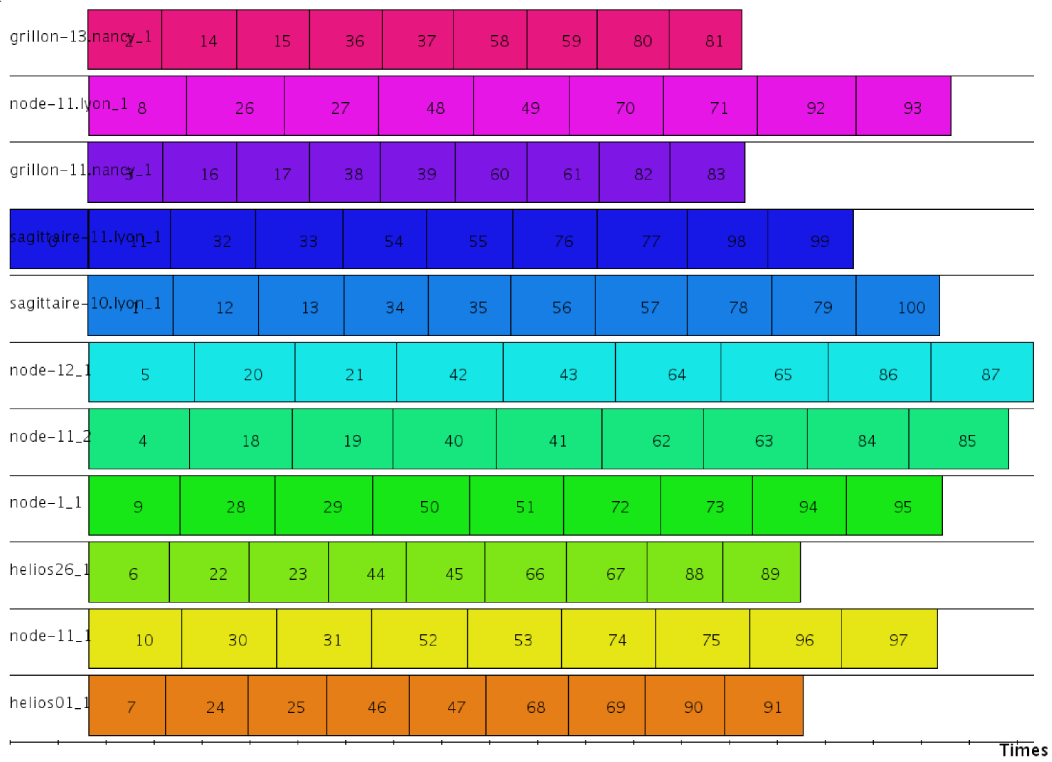
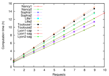
Figure 4: Simulation’s distribution over the SeDs: on the left, the Gantt chart; on the right, the execution time of the 100 sub-simulations for each SeD

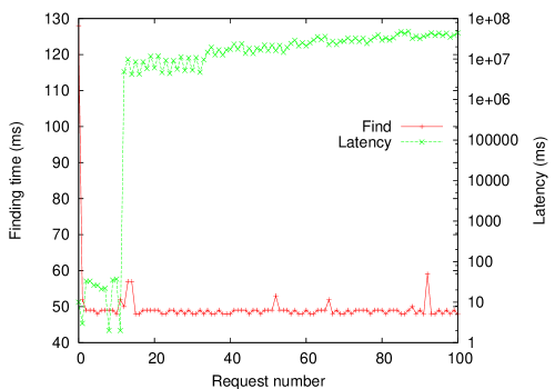
Figure 5: Finding time and latency

6 Conclusion

In this paper, we presented the design of a Diet client and server based on the example of cosmological simulations. As shown by the experiments, Diet is capable of handling long cosmological parallel simulations: mapping them on parallel resources of a grid, executing and processing communication transfers. The overhead induced by the use of Diet is neglectible compared to the execution time of the services. Thus Diet permits to explore new research axes in cosmological simulations (on various low resolutions initial conditions), with transparent access to the services and the data.

References

- [1] E. Caron, F. Desprez, F. Lombard, J.-M. Nicod, M. Quinson, and F. Suter. A Scalable Approach to Network Enabled Servers. In Proceedings of EuroPar 2002, Paderborn, Germany, 2002.
- [2] Andréea Chis, Eddy Caron, Frédéric Desprez, and Alan Su. Plug-in scheduler design for a distributed grid environment. In ACM/IFIP/USENIX, editor, 4th International Workshop on Middleware for Grid Computing - MGC 2006, Melbourne, Australia, November 27th 2006. To appear. In conjunction with ACM/IFIP/USENIX 7th International Middleware Conference 2006.
- [3] A. Denis, C. Perez, and T. Priol. Towards high performance CORBA and MPI middlewares for grid computing. In Craig A. Lee, editor, Proc. of the 2nd International Workshop on Grid Computing, number 2242 in LNCS, pages 14–25, Denver, Colorado, USA, November 2001. Springer-Verlag.
- [4] H. Nakada, M. Sato, and S. Sekiguchi. Design and implementations of ninf: towards a global computing infrastructure. Future Generation Computing Systems, Metacomputing Issue, 15:649–658, 1999.
- [5] R. Teyssier. Cosmological hydrodynamics with adaptive mesh refinement. A new high resolution code called RAMSES. Astronomy and Astrophysics, 385:337–364, 2002.
- [6] R. Teyssier, S. Fromang, and E. Dormy. Kinematic dynamos using constrained transport with high order Godunov schemes and adaptive mesh refinement. Journal of Computational Physics, 218:44–67, October 2006.
- [7] A. YarKhan, K. Seymour, K. Sagi, Z. Shi, and J. Dongarra. Recent developments in gridsolve. In Y eds Robert, editor, International Journal of High Performance Computing Applications (Special Issue: Scheduling for Large-Scale Heterogeneous Platforms), volume 20. Sage Science Press, spring 2006.