Accuracy of slow-roll formulae for inflationary perturbations: implications for primordial black hole formation.

Abstract

We investigate the accuracy of the slow-roll approximation for calculating perturbation spectra generated during inflation. The Hamilton-Jacobi formalism is used to evolve inflationary models with different histories. Models are identified for which the scalar power spectra $\mathcal{P_{R}}$ computed using the Stewart-Lyth slow-roll approximation differ from exact numerical calculations using the Mukhanov perturbation equation. We then revisit the problem of primordial black holes generated by inflation. Hybrid-type inflationary models, in which the inflaton is trapped in the minimum of a potential, can produce blue power spectra and an observable abundance of primordial black holes. However, this type of model can now be firmly excluded from observational constraints on the scalar spectral index on cosmological scales. We argue that significant primordial black hole formation in simple inflation models requires contrived potentials in which there is a period of fast roll towards the end of inflation. For this type of model, the Stewart-Lyth formalism breaks down. Examples of such inflationary models and numerical computations of their scalar fluctuation spectra are presented.

1 Introduction

The simplest models of inflation predict an almost scale-invariant and Gaussian distribution of primordial density perturbations as a consequence of the inflaton field rolling slowly down a potential of a specific form [1, 2]. Provided that the rolling is sufficiently slow, a set of ‘slow-roll’ approximations allows the primordial perturbations to be computed easily.

However, there is no compelling reason why inflation should be of the slow-roll type. Inflationary scenarios that violate the slow-roll conditions have been studied by many authors [3, 4, 5, 6, 7]. Furthermore, observations that constrain the amplitude of primordial perturbations only probe a relatively small range of scales. It is therefore possible that inflation might have been more unusual than that anticipated in the simplest theories, and that there may have been a period of fast roll before inflation ended.

In this paper, we analysed inflationary perturbations numerically for single-field inflationary models with generic evolutionary histories, including cases where slow-roll conditions are badly violated. We then compare the numerical results with those calculated using slow-roll formulae, and identified cases where the two approaches differ.

We revisit the problem of primordial black holes generated by inflation. We argue that primordial black hole formation in slow-roll inflation models is excluded observationally. It is, however, possible to form primordial black holes if there was a period of fast roll towards the end of inflation. For this type of model, numerical computation of the fluctuations is essential to calculate the abundance of primordial black holes. In the final section, we give an explicit example of a model which satisfies observational constraints on CMB scales, but produces primordial black holes in significant abundance. The model is, of course, contrived, but gives an indication of the level of fine-tuning needed to produce primordial black holes in single-field inflation.

2 Evolution of scalar perturbations

2.1 Generating inflationary models

Given our lack of knowledge of the fundamental physics underlying inflation, we shall investigate scalar perturbations in a large number of inflationary models numerically. Our approach is based on the Hamilton-Jacobi formalism introduced in [8]. Tensor perturbations were treated using this formalism in our earlier work [9].

In this approach, the dynamics of inflaton $\phi$ is determined by the Hubble parameter $H(\phi)$, which is related to the potential $V(\phi)$ via the Hamilton-Jacobi equation

$$\left(H^{\prime}(\phi)\right)^{2}-{12\pi\over{m_{\mbox{\scriptsize{Pl}}}^{2}}}H^{2}(\phi)=-{32\pi^{2}\over m_{\mbox{\scriptsize{Pl}}}^{4}}V(\phi)\phantom{t}.$$ (1)

The functional form of $H(\phi)$ can be specified by a hierarchy of ‘flow’ parameters:

$$\epsilon \equiv {m_{\mbox{\scriptsize{Pl}}}^{2}\over 4\pi}\left({H^{\prime}\over H}\right)^{2},\phantom{t}\qquad\qquad\eta\equiv{m_{\mbox{\scriptsize{Pl}}}^{2}\over 4\pi}\left({H^{\prime\prime}\over H}\right)\phantom{t},$$

$$\xi \equiv \left({m_{\mbox{\scriptsize{Pl}}}^{4}\over 16\pi^{2}}\right)\left(H^{\prime}H^{\prime\prime\prime}\over H^{2}\right)\phantom{t},\phantom{t}\phantom{t}\phantom{t}\sigma\equiv 2\eta-4\epsilon\phantom{t},$$ (2)

$${}^{\ell}\lambda_{H}\ \equiv \bigg{(}{m_{\mbox{\scriptsize{Pl}}}^{2}\over 4\pi}\bigg{)}^{\ell}{(H^{\prime})^{\ell-1}\over H^{\ell}}{d^{\ell+1}H\over d^{\ell+1}\phi}\phantom{t},$$

where the definition for the parameter $\sigma$ is motivated by the expression for the scalar spectral index $n_{s}$ [10]

$$n_{s}-1\simeq\sigma-(5-3C)\epsilon^{2}-{1\over 4}(3-5C)\sigma\epsilon+{1\over 2}(3-C)\xi,$$ (3)

with $C=4(\ln 2+\gamma)-5\simeq 0.0814514$. Thus, to lowest order, $\sigma$ describes the departure from scale-invariance.

The flow variables satisfy the following equations (see e.g. [10] and references therein)

$${d\epsilon\over dN} = \epsilon(\sigma+2\epsilon)\phantom{t},$$

$${d\sigma\over dN} = -\epsilon(5\sigma+12\epsilon)+2\xi\phantom{t},$$ (4)

$${d\over dN}\phantom{t}^{\ell}\lambda_{H} = \Big{[}{\ell-1\over 2}\sigma+(\ell-2)\epsilon\Big{]}\phantom{t}^{\ell}\lambda_{H}+\phantom{t}^{\ell+1}\lambda_{H}\phantom{t},\phantom{t}(\ell\geq 2)$$

where $N$ is the number of e-foldings before inflation ends. These flow equations have been used widely in the literature to study inflationary dynamics [11, 12, 13]. For a particular choice of initial conditions for the flow parameters, equations (4) can be integrated until the end of inflation without relying on any slow-roll assumption. In this way one can explore the full dynamics of a large number of simple inflationary models in a relatively model independent way. Nevertheless, in section 4.2, we shall explore another approach to inflation model building based on $\epsilon(N)$.

Having generated a model of inflation, the spectrum of curvature perturbations can be calculated using analytic formulae such as those derived in [14, 15, 16, 17]. In this paper, we shall focus the accuracy of the Stewart-Lyth formula [14], which has been widely used to calculate inflationary perturbations. This approach is not necessarily self-consistent if the conditions of slow roll are violated during inflation (which is, of course, allowed by equations (4)). An alternative approach is to calculate the perturbation spectra numerically using, for example, the Mukhanov formalism [18, 19]. We briefly compare these two approaches.

2.2 The Stewart-Lyth approximation

If the inflaton field $\phi$ rolls so slowly that its kinetic energy is continually dominated by its potential energy, then the power spectrum of scalar curvature perturbations (we consider only scalar perturbations in this paper) can be approximated by the standard first-order slow-roll approximation:

$$\mathcal{P}^{1/2}_{\mathcal{R}}(k)\simeq{2\over m_{\mbox{\scriptsize{Pl}}}^{2}}{H^{2}\over|H^{\prime}|}\Bigg{|}_{k=aH},$$ (5)

where primes denote differentiation with respect to $\phi$. The next order correction is given by Stewart and Lyth [14]

$$\mathcal{P}^{1/2}_{\mathcal{R}}(k)\simeq\left(1-\epsilon+{C-3\over 8}\sigma\right){2\over m_{\mbox{\scriptsize{Pl}}}^{2}}{H^{2}\over|H^{\prime}|}\Bigg{|}_{k=aH},$$ (6)

where $C$ is the constant introduced in equation (3). Equations (5) and (6) are evaluated at the instant when each Fourier mode $k$ crosses the Hubble radius.

For numerical purpose, we express the Stewart-Lyth power spectrum purely in terms of the flow parameters:

$$\!\!\!\!\!\!\!\!\!\!\!\!\!\!\!\!\!\!\!\!\!\mathcal{P}_{\mathcal{R}}(k)\simeq\mathcal{P}_{\mathcal{R}}(k_{0}){\left[1-\epsilon+{C-3\over 8}\sigma\right]^{2}\epsilon^{-1}\bigg{|}_{k=aH}\over\left[1-\epsilon+{C-3\over 8}\sigma\right]^{2}\epsilon^{-1}\bigg{|}_{k_{0}=aH}}\exp\left(-2\int^{\ln|k/k_{0}|}_{0}\epsilon(60-N^{\prime})dN^{\prime}\right),$$ (7)

where $k_{0}=0.002$ Mpc^-1 is the pivot scale at which the spectrum is normalised. This normalisation is estimated as

$$\mathcal{P_{R}}(k_{0}=0.002\mbox{ Mpc}^{-1})\simeq 2.36\times 10^{-9}\phantom{t}.$$ (8)

from the 3-year WMAP results combined with several other datasets [20].

2.3 The Mukhanov formalism

The Stewart-Lyth formula assumes that the background parameters $\epsilon,\sigma$ are approximately constant as each mode crosses the Hubble radius. However, as soon as the inflaton potential becomes steep, $\epsilon$ and $\sigma$ will change rapidly and the formula becomes unreliable. To calculate the curvature spectrum accurately in such cases, we compute a numerical solution for the Mukhanov variable $u$ [18, 19]

$$u=-z\mathcal{R}\phantom{t},\qquad\phantom{t}z={a\over H}{d\phi\over dt}\phantom{t},$$ (9)

where $\mathcal{R}$ is the curvature perturbation. In Fourier space, $u_{k}$ evolves according to a Klein-Gordon equation with a time-varying effective mass:

$${d^{2}u_{k}\over d\tau^{2}}+\left(k^{2}-{1\over z}{d^{2}z\over d\tau^{2}}\right)u_{k}=0,$$ (10)

where $\tau$ is the conformal time $d\tau=dt/a$. At early times $\tau_{i}$, when the mode $k$ is much smaller than the Hubble radius, $u_{k}$ is usually chosen to represent the Bunch-Davies vacuum state with

$$u_{k}(\tau_{i})={1\over\sqrt{2k}}e^{-ik\tau_{i}}.$$ (11)

During inflation, $u_{k}$ evolves in time until the physical scale of each mode is far outside the Hubble radius, at which point $|\mathcal{R}|$ approaches the asymptotic value and freezes. The power spectrum can then be evaluated as:

$$\mathcal{P}_{\mathcal{R}}(k)={k^{3}\over 2\pi^{2}}\left|{u_{k}\over z}\right|_{k\ll aH}^{2}.$$ (12)

To numerically integrate equation (10), we rewrite it in terms of the number of e-foldings $N$ rather than conformal time

$${d^{2}u_{k}\over dN^{2}}-(1-\epsilon){du_{k}\over dN}+\left[\left(k\over aH\right)^{2}-f(\epsilon,\sigma,\xi)\right]u_{k}=0,$$ (13)

since we use the inflationary flow equations to calculate the evolution of the unperturbed background. The factor $f$ in equation (13) is given by

$$f(\epsilon,\sigma,\xi)=2-4\epsilon-{3\over 2}\sigma-2\epsilon^{2}+{\sigma^{2}\over 4}+\xi,$$ (14)

and is exact despite its dependence on the flow variables. The initial conditions assigned to $u_{k}$ are:

$$\mbox{Re}(u_{k}(\tau_{i}))={1\over\sqrt{2k}}\phantom{t},\qquad \left({du_{k}\over dN}(\tau_{i})\right)=0\phantom{t},$$ Re

$$\mbox{Im}\left(u_{k}(\tau_{i})\right)=0\phantom{t},\qquad \left({du_{k}\over dN}(\tau_{i})\right)=-{1\over aH}\sqrt{k\over 2}\phantom{t},$$ Im (15)

where $aH/k$ is a small fixed ratio, which we have set to be $10^{-3}$. We have checked that the final power spectrum shows negligible change if this ratio is reduced further.

For each inflation model, we continue evolving each mode until the end of inflation, so that

$$\mathcal{P}_{\mathcal{R}}(k)=\mathcal{P}_{\mathcal{R}}(k_{0})\left({k\over k_{0}}\right)^{3}\left|{u_{k}\over u_{k_{0}}}\right|^{2}_{\mbox{\scriptsize{end}}}.$$ (16)

As long as inflation satisfies slow-roll conditions ($\epsilon$, $\sigma\ll 1$), the numerical solution (16) will agree accurately with the Stewart-Lyth approximation (6) for all modes that are well outside the horizon at the end of inflation. However, there can be large differences if the slow conditions are violated temporarily during inflation. These types of models have been analysed by Leach et al. [23, 24]. In particular, it was shown in reference [24] that the Stewart-Lyth formula will fail if the quantity $z$ in (9) becomes smaller than its value at the time a mode crosses the Hubble radius. Some specific examples of this behaviour are described in the next section.

3 Limitations of slow-roll approximation

As in previous papers [10, 11, 12] we use the inflationary flow equations (4) to evolve a large number of inflation models with initial flow parameters selected at random from the uniform distributions

$$\epsilon_{0} \in [0,0.8]\phantom{t},$$

$$\sigma_{0} \in [-0.5,0.5]\phantom{t},$$

$$\xi_{0} \in [-0.05,0.05]\phantom{t},$$ (17)

$${}^{\ell}\lambda_{H}|_{0} \in [-0.025\times 5^{-\ell+3},0.025\times 5^{-\ell+3}]\phantom{t},\phantom{t}(3\leq\ell\leq 10)$$

$${}^{11}\lambda_{H}|_{0} = 0\phantom{t}.$$

The distributions (17) should not be interpreted as a physical probability distribution for inflationary models, but merely as a device for generating models with a wide range of evolutionary histories. Despite the fact that the truncation is made at $\ell=11$, the types of models that we generated were sufficiently diverse for us to understand when and why the Stewart-Lyth approximation breaks down in general. Keeping the hierarchy to higher orders can produce more complicated inflationary models, but this will not affect our qualitative conclusions.

We have selected three models for which the Stewart-Lyth approximation differs to varying degrees from integrating equation (10). First, we consider small scale perturbations where the Stewart-Lyth formula is inaccurate for modes for which $|\mathcal{R}|$ does not have time to reach its asymptotic value well before inflation ends. Next, we describe an inflationary scenario where $\epsilon$ changes rapidly, arising from a ‘bumpy’ potential. Finally, we show an example for which the potential has a steep feature, inducing fast roll and interrupting inflation temporarily. Models based on specific potentials $V(\phi)$ displaying similar behavior to each of these three models can be found in [23, 24, 4]. Throughout, we assume that there were $60$ e-folds of inflation between the time CMB scale perturbations were generated and the end of inflation.

3.1 Small-scale perturbations

Figure 1a shows $\epsilon(N)$ for a typical inflationary scenario that lasts for 60 e-folds generated from the distribution (17). Within the last few e-folds of inflation, $\epsilon$ rises rapidly to unity. Consequently, the damping term in equation (13) is suddenly reduced, and $u_{k}$ evolves more like a frictionless oscillator. This results in an upturn in the power spectrum $\mathcal{P_{R}}$ (figure 1b), peaking at the smallest scales that exit the Hubble radius.

Figure 1: Panel (a) shows the parameter $\epsilon$ as a function of $N$, the number of e-folds of inflation (with $N=0$ at the end of inflation). Rise in $\epsilon$ towards unity at the end of inflation gives rise to the small scale feature of the power spectrum $\mathcal{P_{R}}(k)$, shown in panel (b). The spectrum in bold line uses the Mukhanov variable (16) while the thin line shows the Stewart-Lyth approximation (7).

Figure 2: Panel (a) shows $\epsilon(N)$ for a model in which $\epsilon(N)$ peaks prominently during inflation as a consequence of a bumpy potential with a pronounced bump or drop. The origin of the dip in the Mukhanov spectrum (panel (b), bold line) and its magnitude in comparison with that of the Stewart-Lyth spectrum are discussed in the text.

Figure 3: Panel (a) shows $\epsilon(N)$ for a model which temporarily fast-rolls (when $\epsilon>1$), giving rise to a typical ‘ringing’ in the power spectrum shown in panel (b). The origin of the large discrepancy between the Mukhanov (bold) and the Stewart-Lyth spectra in panel (b) is discussed in the text.

The numerical solution of the Mukhanov equation (10) (bold line) and the Stewart-Lyth formula are almost indistinguishable for wavenumbers $k\lesssim 10^{18}$ Mpc^-1 . Deviations in the solutions can be seen at larger wavenumbers, but they are relatively small. This behaviour is quite typical for models in which inflation ends when $\epsilon$ exceeds unity. For most purposes the Stewart-Lyth formula will provide an excellent approximation to the power spectrum even on small scales. Large deviations from the Stewart-Lyth formula require more unusual inflationary models such as the two examples described next.

3.2 ‘Bumpy’ potential

Figure 2a illustrates a scenario in which $\epsilon$ peaks strongly during inflation as result of a potential with a pronounced bump or drop. Here the Stewart-Lyth approximation and the exact integration agree at large scales but differ considerably as the background evolves rapidly leading to the prominent dip in $\mathcal{P_{R}}$ as seen in figure 2b. We can understand this feature as follows. As the background value of $\epsilon$ rises around a potential bump during inflation, the dynamics of the flow variables require that $\sigma$ simultaneously plummets to large negative values. Thus, according to the slow-roll formula for the spectral index (3), the gradient of the power spectrum also decreases to large negative values. This explains the downturn in the Stewart-Lyth spectrum. However, superhorizon evolution, which is neglected by the Stewart-Lyth approximation, becomes important when the background changes rapidly. In this case, as $\sigma$ becomes large and negative, one finds that the Mukhanov variable evolves as $u_{k}\sim e^{-|A|N}$ where $A=O(\sigma)$. This results in an additional decrease in $\mathcal{P_{R}}$ around the bump. Subsequently, towards the true end of inflation, the tail of the spectrum resembles that in figure 1b as expected.

3.3 Fast roll

Consider a scenario in which $\epsilon(N)$ peaks so strongly during inflation that $\epsilon$ exceeds unity temporarily, hence breaking up inflation into two or more stages (see e.g. [25]). Such a ‘fast-roll’ model is shown in figure 3.

The power spectrum resulting from fast roll (figure 3b) shows a large difference between the Mukhanov and the Stewart-Lyth spectra. In addition to the enhanced dip as explained earlier, we draw attention to two other features: i) the subsequent sharp rise of the Mukhanov spectrum several orders of magnitude above the Stewart-Lyth approximation, and ii) the rapid oscillating features across $10^{11}\leq k/\mbox{Mpc}^{-1}\leq 10^{16}$.

These features can be understood as follows. Equation (13) clearly shows what happens to the Mukhanov variable $u_{k}$ during fast roll. The $(1-\epsilon)$ friction term of the harmonic oscillator becomes negative during fast roll, hence boosting $|u_{k}|$ momentarily. Physically, fast-rolling leads to an entropy perturbation which sources growth of curvature perturbations on superhorizon scales [23]. The finer-scale ‘ringing’ induced during fast roll have previously been seen in [6, 4] in their investigations of a potential with a step.

4 Application to primordial black holes

Many authors have speculated on the possible existence of primordial black holes generated during the early Universe [26, 27, 28, 29]. Such objects, if they are more massive than $10^{15}$ g could contribute to the dark matter density at the present time [30, 31] and may be the source of high energy cosmic rays [32, 33] (see [34] for a recent review). However, it has proved difficult to think of compelling scenarios in which an interesting density of primordial black holes could form. Formation of primordial black holes in inflationary models have been discussed by a number of authors (see [35, 36] and especially [37], which is the closest in spirit to this work). We revisit this problem in this section and show that significant primordial black hole formation during inflation could have occured only if the inflationary dynamics were highly unusual and finely tuned. For such unusual inflationary models, an accurate computation of the primordial black hole abundance requires numerical integration of the inflationary perturbations as described in the previous section.

4.1 Basic quantities

Here, we consider black holes that form when inflation ends and primordial density fluctuations begin to re-enter the Hubble radius. In this section we review the basic quantities relevant to the formation of primordial black holes and compute their relic abundance using the Sheth-Tormen mass function [38].

Fluctuations in the energy density smoothed over a spherical region of scale $R$ are related to the energy density field $\delta(\mathbf{x})$ by the convolution

$$\delta(R,\mathbf{x})=\int W(|\mathbf{x^{\prime}}-\mathbf{x}|/R)\delta(\mathbf{x^{\prime}})d^{3}x^{\prime},$$ (18)

where $W$ denotes a ‘window function’ of scale $R$ . In Fourier space, the variance of $\delta(R,\mathbf{x})$ is given by

$$\sigma^{2}(R) = \int_{0}^{\infty}\mathcal{P}_{\delta}(k)\hat{W}^{2}(kR){dk\over k},$$ (19)

where $\hat{W}(kR)$ is the Fourier transform of the window function $W$. Here we will assume that $W$ is a top-hat function of radius $R$ (see e.g. [39], §4.3.3).

The power spectrum of the energy density perturbations $\mathcal{P}_{\delta}(k)={k^{3}/2\pi^{2}}\langle|\delta(k)|^{2}\rangle$ is related to the spectrum of curvature perturbations $\mathcal{P_{R}}(k)$ by [39]:

$$\mathcal{P}_{\delta}(k)\simeq{16\over 81}\left(k\over aH\right)^{4}\mathcal{P_{R}}(k).$$ (20)

A region with density contrast $\delta$ forms a black hole if $\delta$ exceeds a critical value $\delta_{c}$. Previous authors have shown that $\delta_{c}$ should be roughly equal to the equation of state during radiation era $(\delta_{c}\simeq 1/3)$ [28, 40, 41], and we shall take $\delta_{c}=1/3$ throughout this paper. In addition to the lower limit there is an upper bound for $\delta$ of approximately unity, since for such high overdensities large positive curvatures will cause patches to close on themselves, creating disconnected ‘baby’ universes [28].

Next, to obtain the mass spectrum of primordial black holes, consider the mass $M$ associated with a region of comoving size $R$ and average energy density $\rho$. Early work by Carr [45] suggested that primordial black holes form with mass comparable to the ‘horizon mass’, i.e.

$$M\simeq{4\pi\over 3}w^{3/2}\rho\left(H^{-1}\right)^{3}.$$ (21)

Recent numerical investigations [42], however , suggest that $M$ may be a small fraction of the horizon mass, and may be bounded from below [44, 46]. Nevertheless, these results have been criticised by some authors [43], and we shall still use equation (21) in this paper. It then follows that $M$ and $R$ are related by [47]

$${R\over 1\mbox{ Mpc}}\simeq 2.2\times 10^{-24}\left({M\over 1\mbox{ g}}\right)^{1/2}\left({g_{*}\over 2}\right)^{1/12},$$ (22)

where the effective relativistic degree of freedom $g_{*}$ is of order 100 in the very early universe when the temperature exceeds $\sim 300$ GeV. By combining Equations (19)-(22), the variance $\sigma(R)$ can then be converted to the mass variance $\sigma(M)$.

The fraction of the universe, $\Omega_{\mbox{\scriptsize{pbh}}}$, in primordial black holes of mass greater than $M$ is

$$\Omega_{\mbox{\scriptsize{pbh}}}\equiv{\rho_{\mbox{\scriptsize{pbh}}}\over\rho_{\mbox{\scriptsize{total}}}}\simeq\int_{\delta_{c}}^{1}P(\delta(M))d\delta(M),$$ (23)

where $P(\delta)$ is the density fluctuation probability distribution smoothed on scale $M$ and is such a sharply falling function that the upper limit can be extended to infinity without loss of accuracy. Previous work [48, 49, 50] has used the Press-Schechter formalism, in which $P(\delta)$ is a Gaussian function, yielding

$$\Omega_{\mbox{\scriptsize{pbh}}}(>M)=\mbox{erfc}\left(\delta\over\sqrt{2}\sigma(M)\right)$$ (24)

Here we use the Sheth-Tormen mass function [38] which is based on an ellipsoidal model of gravitational collapse and provides a better fit than the Press-Schechter function to the abundances of non-linear structures in numerical simulations [51]. The primordial black hole abundance now becomes:

$$\Omega_{\mbox{\scriptsize{pbh}}}(>M)=\mathcal{A}\left[\mbox{erfc}\left(\sqrt{a\over 2}{\delta_{c}\over\sigma(M)}\right)+{1\over 2^{p}\sqrt{\pi}}\Gamma\left({1\over 2}-p,{a\delta_{c}^{2}\over 2\sigma^{2}(M)}\right)\right],$$ (25)

where $\mathcal{A}\simeq 0.3222$, $p\simeq 0.3$, $a=0.707$ and $\Gamma(x,y)$ is the incomplete gamma function.

4.2 Results

For inflationary models that support primordial black hole production, we calculated the black hole abundance using the Sheth-Tormen formula (25) with $M=10^{15}$g, corresponding to the lightest black holes that may survive till present day without evaporating completely. For models that are radiation dominated at the end of inflation (i.e. do not experience an extended matter dominated phase), the observational constraints on the primordial black hole abundance can be described roughly by

$$\Omega_{\mbox{\scriptsize{pbh}}}(M>10^{15}\;{\rm g})\lesssim 10^{-20}.$$ (26)

More accurately, the constraint on $\Omega_{\mbox{\scriptsize{pbh}}}$ is a function of the mass of the primordial black holes and on the physics of the (p)reheating phase [52, 53]. In this paper it will be adequate to use the simple criterion (26) to give a feel for the types of inflation models that might produce black holes.

4.2.1 Models with blue spectra

A viable model of inflation requires at least $60$ e-folds of inflation [54]. Using the inflationary flow equations, we find that the vast majority of inflationary flow models that experience such a large number of e-folds are models in which the inflaton is trapped in a local minimum of the potential [10, 11]. For such models, inflation never ends unless some additional physical mechanism is included. Examples of such mechanisms include an auxiliary field, as in hybrid inflation [55] or open strings becoming tachyonic in brane inflation models [56]. In these models, the resulting spectrum of curvature perturbation is very well approximated by a power-law relation:

$$\mathcal{P_{R}}(k)=\mathcal{P_{R}}(k_{0})\left(k\over k_{0}\right)^{n_{s}-1},$$ (27)

with spectral index $n_{s}$ given by equation (3). As the inflaton sits in the local minimum, $\epsilon$ remains very small while $\sigma$ is positive and may be large. Thus, the power spectrum for this type of models is ‘blue’ ($n_{s}>1)$. The running of $n_{s}$ is given by

$${dn_{s}\over d\ln k}\simeq-{1\over{1-\epsilon}}\left(2\xi-28\epsilon^{2}-5\epsilon\sigma-\left(3-5C\over 2\right)\epsilon\xi+\left(3-C\over 4\right)\xi\sigma\right).$$ (28)

Because the leading order comes from the small $\xi$ term, the running in these blue models is negligible. Therefore, the shape of the curvature power spectrum in these models can be characterized accurately by a constant spectral index $n_{s}$.

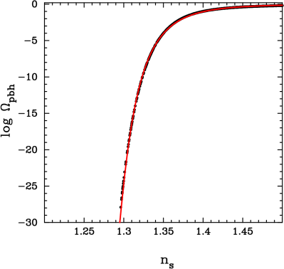
Figure 4: Plot of the primordial black hole abundance $\Omega_{\mbox{\scriptsize{pbh}}}(M>10^{15}$g) against the spectral index $n_{s}$ for $10^{6}$ models where inflation ends suddenly. There is virtually no dispersion around the curve given approximately by equation (29). The exponential sensitivity of $\Omega_{\mbox{\scriptsize{pbh}}}$ on $n_{s}$ at the steep part of the curve highlights the level of fine-tuning needed to produce an interesting density of primordial black hole .

Consequently, for models with blue spectra, $n_{s}$ directly determines the abundance of primordial black holes $\Omega_{\mbox{\scriptsize{pbh}}}$, as shown in Figure 4. The points show models trapped in a local minimum of the potential for which inflation was arbitrarily terminated after 200 e-folds. The curve shows the fitting function

$$\log_{10}\Omega_{\mbox{\scriptsize{pbh}}}=-\alpha\left(1+\left(\beta(n_{s}-1.295)\right)^{p}\right)^{-1/q},$$ (29)

where $\alpha=30$, $\beta=10.2891$, $p=1.05307$ and $q=0.218219$. Thus, the constraint $\Omega_{\mbox{\scriptsize{pbh}}}\lesssim 10^{-20}$ discussed above implies an upper bound in $n_{s}$

$$n_{s}\lesssim 1.3,$$ (30)

in excellent agreement with the analysis of [52], which used constraints on the amplitude of the scalar fluctuations derived from the four-year COBE data [57]. However, the observational constraints from the 3-year WMAP and SDSS [20, 58, 59, 60] can now convincingly exclude a high density of primordial black holes from this type of model (for example, reference [58] quotes $n_{s}=0.964$ with a $1\sigma$ error of only $\pm 0.012$).

4.2.2 Designing potentials with $\epsilon$(N)

The abundance of primordial black holes is closely linked to the power spectrum $\mathcal{P_{R}}(k)$ on small scales. If the power spectrum has a high amplitude at small scales, as in the case of blue spectra described above, a significant density of massive primordial black holes may form. However, using the inflationary flow approach, models that support 60 e-folds of inflation and end with $\epsilon=1$, are in general, tilted ‘red’ over a large range of scales and therefore cannot produce primordial black holes. Even the small upturns seen in figures 1b and 2b occur at such low amplitudes that $\Omega_{\mbox{\scriptsize{pbh}}}$ remains negligible.

However, as discussed in §3.3, for models which experience a period of fast roll, it is possible to generate a large jump in $\mathcal{P_{R}}$ at small scales, and this can lead to primordial black hole production. For such models, it is important to use a numerical computation to calculate the power spectrum rather than the Stewart-Lyth approximation. For example, for the model shown in figure 3, the Stewart-Lyth approximation predicts a negliglble density of primordial black holes whereas integration of the Mukhanov equation gives $\Omega_{\mbox{\scriptsize{pbh}}}(M>10^{15}g)\simeq{10^{-5}}$. One can therefore ask if it is possible to construct fast-roll models that can produce an interesting primordial black hole abundance, while satisfying the current observational constraints on the shape of the power spectrum at large scales.

We can construct such models easily based on the Hamilton-Jacobi approach by specifying the dynamics of inflation in terms of $\epsilon(N)$ . We first choose a set of values of $\epsilon(N)$ with the boundary conditions:

$$\epsilon(0)=1,\qquad\lim_{N\rightarrow\infty}\epsilon=0_{+}.$$ (31)

The observational constraints on $r$, $n_{s}$ and its running can be satisfied by adjusting the values of $\epsilon$, $d\epsilon/dN$ and $d^{2}\epsilon/dN^{2}$ at $N=60$. The form of $\epsilon(N)$ can then be adjusted ‘by hand’ to generate a brief period of fast roll at small values of $N$ to produce a significant density of primordial black holes.

Figure 5: Left panel shows $\epsilon(N)$ designed using Hermite interpolating polynomials. Fast-roll regime has been modelled so as to produce primordial black holes at an interesting abundance. The reconstructed power spectrum $\mathcal{P_{R}}(k)$ is shown in the right panel. For this model, $\Omega_{\mbox{\scriptsize{pbh}}}(M>10^{15}\phantom{t}\mbox{g})\simeq 1.6\times 10^{-20}$. The observables at CMB scales are $r\simeq 0.01$, $n_{s}\simeq 0.99$ and $dn_{s}/d\ln k\simeq 10^{-5}$, broadly compatible with constraints from WMAP and other data.

We then construct $\epsilon(N)$ by using piecewise cubic Hermite interpolating polynomials. These polynomials are well suited for our purposes since it is easy to apply constraints on the positions of extrema and on the derivatives. The values of $\epsilon(N)$ and its first and second derivatives then completely determine the evolution of the Mukhanov variable $u$ via equation (13), and thus the power spectrum $\mathcal{P_{R}}$ can be reconstructed. Figure 5 shows $\epsilon(N)$ for such a fast-roll model and the reconstructed power spectrum. For this model,

$$\Omega_{\mbox{\scriptsize{pbh}}}\simeq 1.6\times 10^{-20},\phantom{t}\phantom{t}\phantom{t}r\simeq 0.01,\phantom{t}\phantom{t}\phantom{t}n_{s}\simeq 0.99,\phantom{t}\phantom{t}\phantom{t}{dn_{s}/d\ln k}\simeq 10^{-5},$$ (32)

and so is broadly compatible with observational constraints [20] yet produces a significant abundance of primordial black hole . It is, of course, possible to generate many variants of this type of model with different values of $n_{s}$ and $dn_{s}/d\ln k$ on CMB scales. But all such models will require a finely tuned period of fast roll towards the end of inflation if they are to produce remnant black holes.

We end this section with a brief comment on the effect of non-gaussianities on primordial black hole abundance. Chen et al. [61] recently pointed out that step-like features in the inflaton potential can give rise to large non-gaussianities in the primordial perturbations. The effect of non-gaussianities on the abundance of primordial black holes was considered in [62, 63]. These authors found that:

$$\Omega_{\mbox{\scriptsize{pbh}}}(>M)\simeq\Omega_{\mbox{\scriptsize{pbh}}}^{\mbox{\scriptsize{Gaussian}}}+\mathcal{G}\exp{\left(-{\delta_{c}^{2}\over\sigma^{2}(M)}\right)},$$ (33)

where $\mathcal{G}=\mathcal{O}(f_{\mbox{\scriptsize{NL}}})$. Thus, even large non-gaussianities anticipated in fast-roll models will be exponentially suppressed, and the overall effect on $\Omega_{\mbox{\scriptsize{pbh}}}$ is expected to be small.

5 Conclusions

There have been many papers discussing the formation of primordial black holes from inflation. The simplest such models involve slow-roll inflation and inflationary dynamics that lead to a blue perturbation spectrum. For this type of model, our results confirm earlier work that shows that the scalar spectral index must be less than $n_{s}\sim 1.3$ to avoid overproduction of primordial black holes. However, we also argue that the most natural way to realise such models is to arrange the inflaton to be trapped in a minimum of a potential and for inflation to end abruptly, as in hybrid inflationary models. For such model, the run in the spectral index and the amplitude of the tensor component is negligible. Therefore, observational constraints on the scalar spectral index determined on CMB scales can be extrapolated to the small scales relevant for primordial black hole production. The strong constraints on the scalar perturbations from WMAP and other data therefore rule out primordial black hole production from slow-roll inflationary models.

It is, however, possible to generate inflationary models which satisfy observational constraints on CMB scales yet produce a significant density of primordial black holes provided there is a period where slow-roll conditions are violated towards the end of inflation. We have shown in section 3 that for this type of model, it is essential to compute the perturbation power spectra numerically, rather than using slow-roll approximations. Section 4.2 presents a construction method for such a model based on designing $\epsilon(N)$. While it is possible to produce primordial black holes from inflation, the dynamics of this type of fast-roll model must be very finely-tuned to produce an acceptable density of primordial black holes. In general, even if a model is constructed to have a period of fast roll, the primordial black hole density will either be excessively high or negligible. Although there has been renewed interest in primordial black holes as a possible explanation for the existence of intermediate mass black holes [64], and to account for the rapid growth of supermassive black holes in the centres of galaxies [65], it seems extremely unlikely to us that primordial black holes formed as a result of inflationary dynamics.

References

References

- [1] A. Albrecht and P. J. Steinhardt. Cosmology for grand unified theories with radiatively induced symmetry breaking. Phys. Rev. Lett., 48:1220, 1982.
- [2] A. D. Linde. Chaotic inflation. Phys. Lett., B129:177, 1983.
- [3] A. D. Linde. Fast-roll inflation. JHEP, 11:052, 2001.
- [4] J. A. Adams, B. Cresswell, and R. Easther. Inflationary perturbations from a potential with a step. Phys. Rev., D64:123514, 2001.
- [5] K. Dimopoulos and D. H. Lyth. Models of inflation liberated by the curvaton hypothesis. Phys. Rev., D69:123509, 2004.
- [6] A. A. Starobinsky. Spectrum of adiabatic perturbations in the universe when there are singularities in the inflaton potential. JETP. Lett., 55:489, 1992.
- [7] T. Matsuda. Elliptic inflation: Generating the curvature perturbation without slow-roll. JCAP, 0609:003, 2006.
- [8] M. B. Hoffman and M. S. Turner. Kinematic constraints to the key inflationary observables. Phys. Rev., D64:023506, 2001.
- [9] S. Chongchitnan and G. Efstathiou. Prospects for direct detection of primordial gravitational waves. Phys. Rev., D73:083511, 2006.
- [10] W. H. Kinney. Inflation: Flow, fixed points and observables to arbitrary order in slow roll. Phys. Rev., D66:083508, 2002.
- [11] S. Chongchitnan and G. Efstathiou. Dynamics of the inflationary flow equations. Phys. Rev., D72:083520, 2005.
- [12] A. R. Liddle. On the inflationary flow equations. Phys. Rev., D68:103504, 2003.
- [13] H. V. Peiris et al. First year wilkinson microwave anisotropy probe (wmap) observations: Implications for inflation. Astrophys. J. Suppl., 148:213, 2003.
- [14] E. D. Stewart and D. H. Lyth. A more accurate analytic calculation of the spectrum of cosmological perturbations produced during inflation. Phys. Lett. B, 302:171, 1993.
- [15] J.-O. Gong and E. D. Stewart. The density perturbation power spectrum to second-order corrections in the slow-roll expansion. Phys. Lett., B510:1, 2001.
- [16] J. Martin and D. J. Schwarz. Wkb approximation for inflationary cosmological perturbations. Phys. Rev., D67:083512, 2003.
- [17] S. Habib, K. Heitmann, G. Jungman, and C. Molina-Paris. The inflationary perturbation spectrum. Phys. Rev. Lett., 89:281301, 2002.
- [18] V. F. Mukhanov. Quantum theory of gauge-invariant cosmological perturbations. Sov. Phys. JETP, 67:1297, 1988.
- [19] M. Sasaki. Large scale quantum fluctuations in the inflationary universe. Prog. Theor. Phys., 76:1036, 1986.
- [20] D. N. Spergel et al. Wilkinson microwave anisotropy probe (wmap) three year results: Implications for cosmology. 2006.
- [21] R. Easther, B. R. Greene, W. H. Kinney, and G. Shiu. Inflation as a probe of short distance physics. Phys. Rev., D64:103502, 2001.
- [22] U. H. Danielsson. A note on inflation and transplanckian physics. Phys. Rev., D66:023511, 2002.
- [23] S. M. Leach and A.R. Liddle. Inflationary perturbations near horizon crossing. Phys. Rev., D63:043508, 2001.
- [24] S. M. Leach, M. Sasaki, D. Wands, and A. R. Liddle. Enhancement of superhorizon scale inflationary curvature perturbations. Phys. Rev., D64:023512, 2001.
- [25] C. P. Burgess, R. Easther, A. Mazumdar, D.F. Mota, and T. Multamaki. Multiple inflation, cosmic string networks and the string landscape. JHEP, 0505:067, 2005.
- [26] S. Hawking. Gravitationally collapsed objects of very low mass. Mon. Not. Roy. Astron. Soc., 152:75, 1971.
- [27] Ya. B. Zeldovich and I.D. Novikov. The hypothesis of cores retarded during expansion and the hot cosmological model. Sov. Astron. A.J., 10:602, 1967.
- [28] B. J. Carr and S. W. Hawking. Black holes in the early universe. Mon. Not. R. Astr. Soc., 168:399, 1974.
- [29] M. Y. Khlopov and A. G. Polnarev. Primordial black holes as a cosmological test of grand unification. Physics Letters B, 97:383, December 1980.
- [30] N. Afshordi, P. McDonald, and D. N. Spergel. Primordial black holes as dark matter: The power spectrum and evaporation of early structures. Astrophys. J., 594:L71, 2003.
- [31] D. Blais, C. Kiefer, and D. Polarski. Can primordial black holes be a significant part of dark matter? Phys. Lett., B535:11, 2002.
- [32] B. J. Carr and J. H. MacGibbon. Cosmic rays from primordial black holes and constraints on the early universe. Phys. Rept., 307:141, 1998.
- [33] A. Barrau, G. Boudoul, and L. Derome. An improved gamma-ray limit on the density of pbhs. 2003.
- [34] B. J. Carr. Primordial black holes: Do they exist and are they useful? 2005.
- [35] B. J. Carr and James E. Lidsey. Primordial black holes and generalized constraints on chaotic inflation. Phys. Rev., D48:543, 1993.
- [36] J. Yokoyama. Formation of Primordial Black Holes in Inflationary Cosmology. Progress of Theoretical Physics Supplement, 136:338, 1999.
- [37] S. M. Leach, I. J. Grivell, and A. R. Liddle. Black hole constraints on the running mass inflation model. Phys. Rev., D62:043516, 2000.
- [38] R. K. Sheth and G. Tormen. Large scale bias and the peak background split. Mon. Not. Roy. Astron. Soc., 308:119, 1999.
- [39] A. R. Liddle and D. H. Lyth. Cosmological inflation and large-scale structure. Cambridge University Press, Cambridge, 2000.
- [40] B. J. Carr. The primordial black hole mass spectrum. Ap. J., 201:1, 1975.
- [41] D. K. Nadezhin, I. D. Novikov, and Polnarev A.G. The hydrodynamics of primordial black hole formation. Sov. Astron., 22:129, 1978.
- [42] J. C. Niemeyer and K. Jedamzik. Dynamics of primordial black hole formation. Phys. Rev., D59:124013, 1999.
- [43] I. Musco, J. C. Miller, and L. Rezzolla. Computations of primordial black hole formation. Class. Quant. Grav., 22:1405, 2005.
- [44] I. Hawke and J. M. Stewart. The dynamics of primordial black-hole formation. Class. Quantum Grav., 19:3687, 2002.
- [45] B. J. Carr. Observational and theoretical aspects of relativistic astrophysics and cosmology. (Sanz, J. L. and Goicoechea, L.J. eds.), World Scientific, Singapore, 1985.
- [46] J. R. Chisholm. Primordial black hole minimum mass. Phys. Rev., D74:043512, 2006.
- [47] P. P. Avelino. Primordial black hole abundance in non-gaussian inflation models. Phys. Rev. D., 72:124004, 2005.
- [48] D. Blais, T. Bringmann, C. Kiefer, and D. Polarski. Accurate results for primordial black holes from spectra with a distinguished scale. Phys. Rev., D67:024024, 2003.
- [49] T. Bringmann, C. Kiefer, and D. Polarski. Primordial black holes from inflationary models with and without broken scale invariance. Phys. Rev., D65:024008, 2002.
- [50] Y. Sendouda, S. Nagataki, and K. Sato. Mass spectrum of primordial black holes from inflationary perturbation in the randall-sundrum braneworld: A limit on blue spectra. JCAP, 0606:003, 2006.
- [51] R. K. Sheth, H. J. Mo, and G. Tormen. Ellipsoidal collapse and an improved model for the number and spatial distribution of dark matter haloes. Mon. Not. Roy. Astron. Soc., 323:1, 2001.
- [52] A. M. Green and A. R. Liddle. Constraints on the density perturbation spectrum from primordial black holes. Phys. Rev., D56:6166, 1997.
- [53] A. M. Green and K. A. Malik. Primordial black hole production due to preheating. Phys. Rev., D64:021301, 2001.
- [54] A. R. Liddle and S. M. Leach. How long before the end of inflation were observable perturbations produced? Phys. Rev., D68:103503, 2003.
- [55] D. H. Lyth and A. Riotto. Particle physics models of inflation and the cosmological density perturbation. Phys. Rept., 314:1, 1999.
- [56] S. Sarangi and S.-H.H. Tye. Cosmic string production towards the end of brane inflation. Phys. Lett., B536:185, 2002.
- [57] C. L. Bennett et al. 4-year cobe dmr cosmic microwave background observations: Maps and basic results. Astrophys. J., 464:L1, 1996.
- [58] U. Seljak, A. Slosar, and P. McDonald. Cosmological parameters from combining the lyman-alpha forest with cmb, galaxy clustering and sn constraints. 2006.
- [59] W. H. Kinney, E. W. Kolb, A. Melchiorri, and A. Riotto. Inflation model constraints from the wilkinson microwave anisotropy probe three-year data. Phys. Rev., D74:023502, 2006.
- [60] H. Peiris and R. Easther. Recovering the inflationary potential and primordial power spectrum with a slow roll prior: Methodology and application to wmap 3 year data. JCAP, 0607:002, 2006.
- [61] X-g. Chen, R. Easther, and E. A. Lim. Large non-gaussianities in single field inflation. 2006.
- [62] D. Seery and J. C. Hidalgo. Non-gaussian corrections to the probability distribution of the curvature perturbation from inflation. JCAP, 0607:008, 2006.
- [63] J.-C. Hidalgo. To be published.
- [64] K. J. Mack, J P. Ostriker, and M. Ricotti. Growth of structure seeded by primordial black holes. 2006.
- [65] N. Düchting. Supermassive black holes from primordial black hole seeds. Phys. Rev., D70:064015, 2004.