Effects of Destriping Errors on CMB Polarisation Power Spectra and and Pixel Noise Covariances

Abstract

Low frequency detector noise in CMB experiments must be corrected to produce faithful maps of the temperature and polarization anisotropies. For a Planck-type experiment the low frequency noise corrections lead to residual stripes in the maps. Here I show that for a ring torus and idealised detector geometry it is possible to calculate analytically the effects of destriping errors on the temperature and polarization power spectra. It is also possible to compute the pixel-pixel noise covariances for maps of arbitrary resolution. The analytic model is compared to numerical simulations using a realistic detector and scanning geometries. We show that Planck polarization maps at $143$GHz should be signal dominated on large scales. Destriping errors are the dominant source of noise for the temperature and polarization power spectra at multipoles $\ell\lower 2.15277pt\hbox{$\;\buildrel<\over{\sim}\;$}10$. A fast Monte-Carlo method for characterising noise, including destriping errors, is described that can be applied to Planck. This Monte-Carlo method can be used to quantify pixel-pixel noise covariances and to remove noise biases in power spectrum estimates.

Key words: Methods: data analysis, statistical; Cosmology: cosmic microwave background, large-scale structure of Universe

1 Introduction

This is the fourth in a series of papers (Efstathiou 2004, 2005, 2006; henceforth E04, E05, E06 respectively) outlining a methodology for analysing power spectra for a Planck-type cosmic microwave background (CMB) experiment. The first of these papers discussed fast hybrid methods for estimating temperature power spectra. The hybrid method combines a maximum likelihood estimator at low multipoles, computed from low resolution maps, with a pseudo-$C_{\ell}$ (PCL) estimator at high multipoles computed using fast spherical transforms applied to high resolution maps (see Hivon et al. 2002 and references therein). A near optimal hybrid estimator can be constructed if the noise properties of the input maps obey certain properties, e.g. if the noise is accurately white at high multipoles and if correlated noise can be accounted for in the pixel-pixel noise covariance matrices for the low resolution maps used in the maximum likelihood estimate. If this is the case, accurate analytic expressions for the PCL covariance matrices can be derived for realistic sky cuts. The hybrid estimator concept was generalised to polarization in E06 and analytic formulae for PCL polarization power spectra for noise-free and noisy data were derived. (See also the related paper by Challinor and Chon, 2005). There is a large literature on power spectrum estimation methods and we will not attempt to give a comprehensive bibliography here. A fairly complete set of references to previous work can be found in the papers of hybrid power spectrum estimators (E04, E06).

CMB temperature map reconstruction errors for a Planck-type were considered in E05, on the assumption that maps would be constructed using simple ‘destriping’ techniques (see e.g. Burigana et al. 1997; Delabrouille 1998; Maino et al. 1999; Revenu et al. 2000; Keihänen et al. 2004, 2005). Destriping algorithms are particularly suited to a Planck-type scanning strategy in which the sky is scanned many times on rings. In E05, it was shown that for a ring torus scanning geometry (and provided the instrument noise satisfies certain reasonable properties) it is possible to compute accurately the effects of residual striping errors on the temperature power spectrum. For realistic detector noise, the resulting error power spectrum is indeed accurately white at high multipoles, but at low multipoles the striping errors introduce a bias in the temperature power spectrum that has a distinctive ‘sawtooth’ type pattern with an envelope that varies approximately as $1/\ell$. For realistic Planck-type scanning geometries, the ring torus model provides a good (but not exact) description of the error power spectrum determined from simulations of the time-ordered data (TOD). E05 also argued that for a slowly precessing scanning strategy, and detector noise properties such as envisaged for Planck, a simple destriping map making algorithm will be close to optimal. The destriping errors are dominated by ‘irreducable’ white noise errors in the ring overlaps and so there is little to be gained by implementing computationally demanding least squares map making methods (e.g. Wright et al. 1996; Tegmark 1997a,b; Borrill et al. 2001; Natoli et al. 2001; Doré et al. 2001). This conjecture has been verified by Ashdown et al. (2006, hereafter A06), who compared a number of map making codes applied to simulated Planck data (specifically, simulations of four 217 GHz detectors). The temperature power spectrum residuals from the different codes are almost identical, except for small differences at low multipoles. A simple destriping code (for example, the Springtide code described by A06) fitting one offset (or ‘baseline’) per ring pointing produces a map that is very close to optimal. Depending on the value of the detector noise ‘knee frequency’, the accuracy of a destriping algorithm can be improved further by increasing the number of baselines and by applying more sophisticated destriping algorithms that include information on the correlations between baseline offsets (Keihänen, Kurki-Suonio and Poutanen, 2005). However, the simulations of A06 show that for the knee frequencies expected for Planck the improvements in the maps are minor as the number of baselines is increased above one per scanning ring.

In this paper we extend the analysis of E05 to polarization. As we will show in Section 3, for a ring torus geometry it is possible to construct an analytic model for temperature and polarization destriping errors. Formulae are presented in Section 3 for the contribution of residual destriping errors to the temperature and polarization power spectra and also for the pixel-pixel noise covariances in maps of arbitrary resolution.

Section 4 describes numerical simulations of a Planck-like focal plane geometry and slow precessing scanning strategy. Specifically, we use the geometry of the four polarization sensitive bolometer pairs at $143$ GHz (see SPP05). However, to make large numbers (thousands) of simulations feasible, we have assumed $60^{\prime}$ FWHM beams instead of the $7.1^{\prime}$ beams of Planck, and that the scans consist of $1080$ ring pointings instead of the $8640$ ring pointings of Planck. The detector white noise assumed for these simulations was adjusted so that the noise properties of the maps match those expected from Planck at equivalent spatial resolution. These simulations therefore give a good impression of the actual noise properties of Planck $143$GHz maps at low multipoles. With these simulations it is possible to compute the pixel-pixel noise covariance matrix for degraded resolution maps and to isolate the component arising from destriping errors. These pixel noise covariance matrices can be compared with the ring torus approximation derived in Section 3. We then develop an extremely fast and accurate Monte-Carlo method of estimating the pixel-pixel noise covariance matrices based on the statistical properties of destriping baseline offsets. This method offers a reliable way of quantifying the pixel-pixel covariance matrices for temperature and polarization maps of arbitrary resolution and for realistic noise and scanning geometries. These pixel-pixel noise covariance estimates can then be used as inputs to maximum likelihood methods of power-spectrum estimation (E04, E06, Slosar and Seljak 2004) or map-based Gibbs sampling methods (see e.g. Larson et al. 2006).

2 Overview of Polarisation Map Making with Destriping

We follow the notation of Keihänen et al. (2005, hereafter KKP05) and write the TOD stream as

$${\bf y}={\bf P}{\bf m}+{\bf n^{\prime}},$$ (1)

where ${\bf m}$ is the pixelised CMB temperature map, ${\bf P}$ is a pointing matrix, and ${\bf n^{\prime}}$ is the detector noise. (Polarized maps will be dealt with below, but to keep the equations simple we will assume for the moment that we are solving for a temperature map). We assume that the noise can be decomposed into a correlated part consisting of a linear combination (described by the matrix ${\bf F}$) of a set of baseline offsets ${\bf a}$ and a white noise component ${\bf n}$,

$${\bf n^{\prime}}={\bf F}{\bf a}+{\bf n},$$ (2)

with covariance matrix

$$\langle{\bf n^{\prime}}({\bf n^{\prime}})^{T}\rangle={\bf F}{\bf C}_{a}{\bf F}^{T}+{\bf C}_{n},\qquad{\bf C}_{a}=\langle{\bf a}{\bf a^{T}}\rangle,\qquad{\bf C}_{n}=\langle{\bf n}{\bf n^{T}}\rangle.$$ (3)

As shown in KKP05, if the distributions of the offsets ${\bf a}$ and white noise ${\bf n}$ are assumed to be Gaussian, the maximimum likelihood map and offsets are give by minimising the $\chi^{2}$,

$$\chi^{2}=({\bf y}-{\bf F}{\bf a}-{\bf P}{\bf m})^{T}{\bf C}_{n}^{-1}({\bf y}-{\bf F}{\bf a}-{\bf P}{\bf m})+{\bf a}^{T}{\bf C}_{a}^{-1}{\bf a},$$ (4)

giving the solutions

$${\bf m} = ({\bf P}^{T}{\bf C}_{n}^{-1}{\bf P})^{-1}{\bf P}^{T}{\bf C}_{n}^{-1}({\bf y}-{\bf F}{\bf a}),$$ (5a)

$${\bf a} = ({\bf F}^{T}{\bf C}_{n}^{-1}{\bf Z}{\bf F}+{\bf C}_{a}^{-1})^{-1}{\bf F}^{T}{\bf C}_{n}^{-1}{\bf Z}{\bf y},$$ (5b)

where

$${\bf Z}={\bf I}-{\bf P}({\bf P}^{T}{\bf C}_{n}^{-1}{\bf P})^{-1}{\bf P}^{T}{\bf C}_{n}^{-1}.$$ (5c)

The Fisher matrix of the baseline offsets is given by the second derivative of (4) with respect to the baselines ${\bf a}$,

$${\bf F}_{a}=({\bf F}^{T}{\bf C}^{-1}_{n}{\bf Z}{\bf F}+{\bf C}_{a}^{-1}),$$ (6)

and we will assume that the posterior distribution of the offsets ${\bf a}$ is given by a Gaussian distribution of the form

$$(2\pi|{\bf F}_{a}^{-1}|)^{-1/2}{\rm exp}\left(-{1\over 2}{\bf a}^{T}{\bf F}_{a}{\bf a}\right).$$ (7)

The first term in (6) depends only on the scanning geometry and white noise component of the detector noise. The second term depends on the form of the detector noise spectrum at low frequencies. For Planck-like noise properties (detector knee frequencies of $\lower 2.15277pt\hbox{$\;\buildrel<\over{\sim}\;$}30$mHz), the first term is dominant and represents an irreducible contribution to the baseline offset covariance. In the rest of this paper we will assume that the irreducible term dominates and hence that the striping errors are independent of the exact form of the low frequency noise spectrum. In other words, we ignore ${\bf C}_{a}$ and assume white noise errors in the TOD throughout. This should be an excellent approximation for Planck (see Figure 5 of E04). It is straighforward to generalise to the results of this paper include correlations ${\bf C}_{a}$ in the baseline offsets. Methods for estimating ${\bf C}_{a}$ from the TOD are discussed in KKP05.

The generalisation of the above analysis to polarization sensitive detectors is straightforward. Define ${\bf y}^{d}$ to be the TOD for detector $d$ with orientation $\alpha^{d}$ with respect to a fixed spherical polar coordinate system. In terms of the Stokes parameters $I$, $Q$ and $U$ in this fixed coordinate system, the detector response is

$${\bf y}^{d}={1\over 2}\left({\bf I}+{\bf Q}\cos(2\alpha^{d})+{\bf U}\sin(2\alpha^{d})\right)+{\bf n^{\prime}},$$ (8)

(see Figure 1 and Section 3.1 for a precise definition of the angle $\alpha$). If the noise covariance ${\bf C}_{n}$ is diagonal, $C_{n}\equiv\sigma_{d}^{2}$ and the pointing matrix $P$ is consists of ones and zeros (denoting when a map pixel falls onto an element of the TOD) the first term in equation (4) can be written as

$$\tilde{\chi}^{2}=\sum_{pd}\sum_{di\subset p}{(y^{d}_{i}-(Fa)_{i}-\hat{y}^{d}_{i})^{2}\over\sigma_{d}^{2}},$$ (9)

where $p$ denotes the map pixel, $di\subset p$ denotes the TOD elements of detector $d$ that lie within map pixel $p$ and $\hat{y}^{d}_{i}$ is the expected TOD signal for detector $d$ from the best fitting maps, $I_{p}$, $Q_{p}$, $U_{p}$, derived by minimising the $\chi^{2}$ of equation (4). If correlated errors are small, the second derivative of (9) gives the inverse covariance matrix for $I_{p}$, $Q_{p}$, $U_{p}$, at pixel $p$,

$${\bf M}_{p}=\left(\begin{array}[]{ccc}\sum{1\over\sigma_{d}^{2}}&\sum{\cos(2\alpha^{d}_{i})\over\sigma_{d}^{2}}&\sum{\sin(2\alpha^{d}_{i})\over\sigma_{d}^{2}}\\ \sum{\cos(2\alpha^{d}_{i})\over\sigma_{d}^{2}}&\sum{\cos^{2}(2\alpha^{d}_{i})\over\sigma_{d}^{2}}&\sum{\cos(2\alpha^{d}_{i})\sin(2\alpha^{d}_{i})\over\sigma_{d}^{2}}\\ \sum{\sin(2\alpha^{d}_{i})\over\sigma_{d}^{2}}&\sum{\cos(2\alpha^{d}_{i})\sin(2\alpha^{d}_{i})\over\sigma_{d}^{2}}&\sum{\sin^{2}(2\alpha^{d}_{i})\over\sigma_{d}^{2}},\end{array}\right),$$ (13)

where the sums extend over all detector TOD elements $di\subset p$. The condition number of the matrix $M$ is often used to determine whether the Stokes parameters are well constrained in map pixel $p$ (see e.g. A06). Evidently, equation (13) applies only if the TOD noise is strictly white and in general the noise will be correlated. Section 4 describes a fast Monte-Carlo method for estimating these correlated errors.

3 Analysis of a Ring Torus

3.1 Ring torus geometry

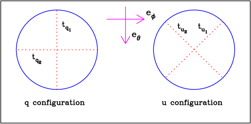
Figure 1: Polarization orientations for two pairs of bolometers in the standard $Q$ and $U$ configurations as discussed in Section 3.1. The polarization angles $\alpha$ for arbitrary detector orientation are defined with respect to the unit vectors $\hat{e}_{\phi}$ and $\hat{e}_{\theta}$ defined with respect to a reference spherical coordinate system.

In this Section, we analyse destriping errors in the idealised case of ring torus scanning geometry with two pairs of bolometers in the ‘standard’ $Q$ and $U$ configurations shown in Figure 1. Each detector pair is assumed to point to the same spot on the sky at a boresight angle of $\theta_{b}$ to the spin axis. The sky is covered by a ring torus composed of a set of discrete $N_{\rm ring}=2\pi/\Delta\alpha$ rings of width $\Delta\alpha$ as the spin axis is repointed along a great circle. The detector orientations of the $Q$- and $U$-configurations with respect to a fixed polarization basis on the sky can be specified by the the angles

$$\alpha^{q}=\cos^{-1}(-\hat{\bf q}_{1}\cdot\hat{\bf e}_{\phi}),\quad\alpha^{u}=\cos^{-1}(-\hat{\bf u}_{1}\cdot\hat{\bf e}_{\phi})-{\pi\over 4}.$$ (14)

Since the detectors are assumed to point to the same spot on the sky, $\alpha^{q}=\alpha^{u}$ for detectors in the standard configuration of Figure 1, though below we will write down general results for arbitrary angles. The response of each of the detectors is denoted $t^{i}_{q_{1}}$, $t^{i}_{q_{2}}$, $t^{i}_{u_{1}}$, $t^{i}_{u_{2}}$, as shown in Figure 1. If the noise in each TOD is white, with identical variance $\sigma^{2}_{d}$, unbiased $I$, $Q$, and $U$ maps can be constructed by minimising (9):

$$I_{p} = \sum_{i\subset p}{1\over 2}(t^{i}_{q_{1}}+t^{i}_{q_{2}}++t^{i}_{u_{1}}+t^{i}_{u_{2}}),$$ (15a)

$$Q_{p} = {S_{2}^{p}(C_{q}^{p}-S_{u}^{p})-S_{3}^{p}(S_{q}^{p}+C_{u}^{p})\over\left(S_{1}^{p}S_{2}^{p}-(S_{3}^{p})^{2}\right)},$$ (15b)

$$U_{p} = {S_{1}^{p}(S_{q}^{p}-C_{u}^{p})-S_{3}^{p}(C_{q}^{p}-S_{u}^{p})\over\left(S_{1}^{p}S_{2}^{p}-(S_{3}^{p})^{2}\right)},$$ (15c)

where

$$C_{\{q,u\}}^{p} = \sum_{i\subset p}(t^{i}_{{\{q,u\}}_{1}}-t^{i}_{{\{q,u\}}_{2}})\cos(2\alpha^{\{q,u\}}_{i}),$$ (16a)

$$S_{\{q,u\}}^{p} = \sum_{i\subset p}(t^{i}_{{\{q,u\}}_{1}}-t^{i}_{{\{q,u\}}_{2}})\sin(2\alpha^{\{q,u\}}_{i}),$$ (16b)

$$S^{p}_{1} = \sum_{i\subset p}(\cos^{2}2\alpha^{q}_{i}+\sin^{2}2\alpha^{u}_{i}),$$ (16c)

$$S^{p}_{2} = \sum_{i\subset p}(\sin^{2}2\alpha^{q}_{i}+\cos^{2}2\alpha^{u}_{i}),$$ (16d)

$$S^{p}_{3} = \sum_{i\subset p}(\cos 2\alpha^{q}_{i}\sin 2\alpha^{q}_{i}-\cos 2\alpha^{u}_{i}\sin 2\alpha^{u}_{i}).$$ (16e)

The problem that we wish to solve in this Section is as follows: Assume that destriping is performed by fitting a single baseline offset for each scanning ring for each detector and assume further that the errors in the baseline offsets are uncorrelated and charaterised by dispersions $\sigma^{2}_{q}$ and $\sigma^{2}_{u}$ for the $Q$- and $U$-configurations respectively. We wish to calculate the biases in the temperature and polarization power spectra associated with these errors. This provides a good model for the effects of residual striping errors on CMB power spectra. As we will show in the rest of this Section, this problem can be solved analytically for a ring torus geometry.

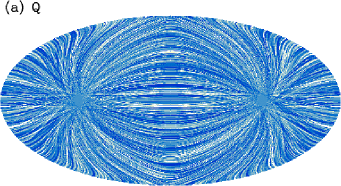
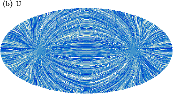
Figure 2: Q and U maps generated from random striping errors for two polarization detector pairs in the standard configuration of Figure 1 and a ring torus scanning geometry with a boresight angle of $\theta_{b}=85^{\circ}$.

To compare with the analytic calculations, we have run a set of $10000$ simulations constructing $I$, $Q$ and $U$ maps, using equations (15a– 15c) for a ring torus geometry with random ring offsets. $Q$ and $U$ maps for one such realisation are shown in Figure 2. In this set of simulations, we use $N_{\rm ring}=2160$ rings of width $\Delta\alpha=2\pi/N_{\rm ring}$ composed of $N_{\rm ring}$ ring pixels. Maps were constructed using an igloo pixelisation scheme (E04) with pixels of size $\Delta\theta_{c}=0.25^{\circ}$. We will refer to these maps as ‘error maps’.

The assumptions underlying these simulations are, of course, highly idealized. As mentioned above, with these assumptions the error power spectra can be computed analytically. It is straightforward to generalise these simulations to realistic Planck-like scanning strategies and to include correlations between (an arbitrary number) of baseline offsets. Simulations of this sort are described in Section 4. As we will show, the Planck scanning strategy (see SPP05) is so close to a ring torus that the model described in the next Section provides quite a good description of the destriping errors expected for Planck.

3.2 Error power spectra

The spherical harmonic transforms of the error maps can be written as

$$a^{T}_{\ell m} = \sum_{ik}w_{ik}\Omega_{ik}I_{ik}Y^{*}_{\ell m}(\theta_{ik},\phi_{ik}),$$ (17a)

$$a^{E}_{\ell m} = -{1\over 2}\sum_{ik}w_{ik}\Omega_{ik}(Q_{ik}R^{+*}_{\ell m}+iU_{ik}R^{-*}_{\ell m}),$$ (17b)

$$a^{B}_{\ell m} = {i\over 2}\sum_{ik}w_{ik}\Omega_{ik}(Q_{ik}R^{-*}_{\ell m}+iU_{ik}R^{+*}_{\ell m}),$$ (17c)

where

$$R^{+}_{\ell m}=\;_{2}Y_{\ell m}+\;_{-2}Y_{\ell m},\qquad R^{-}_{\ell m}=\;_{2}Y_{\ell m}-\;_{-2}Y_{\ell m}.$$ (18)

In these equations the index $k$ denotes the ring number, $i$ denotes the pixel number within the ring and $\Omega_{ik}$ is the solid angle of the ring pixel. $I_{ik}$ is the total intensity in ring $k$, and $Q_{ik}$ and $U_{ik}$ are the Stokes parameters in ring $k$ defined with respect to a fixed polarization basis. The weight factors $w_{ik}$ account for the averaging of the ring pixels in constructing the map and thus are proportional to the inverse of the ‘hit count’ distribution for the ring torus scanning strategy. It is useful to define the auxiliary functions $\hat{P}_{\ell m}$, $\hat{G}^{+}_{\ell m}$ and $\hat{G}^{-}_{\ell m}$:

$$Y_{\ell m} = A^{m}_{\ell}P^{m}_{\ell}(\cos\theta)e^{im\phi}\equiv\hat{P}_{\ell m}e^{im\phi},$$ (19a)

$$R^{+}_{\ell m} = 2\sqrt{2}N_{\ell}A_{\ell}^{m}G^{+}_{\ell m}e^{im\phi}\equiv\hat{G}^{+}_{\ell m}e^{im\phi},$$ (19b)

$$R^{-}_{\ell m} = -2\sqrt{2}N_{\ell}A_{\ell}^{m}G^{-}_{\ell m}e^{im\phi}\equiv\hat{G}^{-}_{\ell m}e^{im\phi},$$ (19c)

where

$$A_{\ell}^{m} = \left({2\ell+1\over 4\pi}{(\ell-m)!\over(\ell+m)!}\right)^{1/2},$$ (20a)

$$N_{\ell} = \left({2(\ell-2)!\over(\ell+2)!}\right)^{1/2},$$ (20b)

and the functions $G^{+}_{\ell m}$ and $G^{-}_{\ell m}$ are

$$G^{+}_{\ell m} = -\left({\ell-m^{2}\over\sin^{2}\theta}+{1\over 2}\ell(\ell-1)\right)P_{\ell}^{m}(\cos\theta)+(\ell+m){\cos\theta\over\sin^{2}\theta}P_{\ell-1}^{m}(\cos\theta),$$ (21a)

$$G^{-}_{\ell m} = {m\over\sin^{2}\theta}\left\{(\ell-1)\cos\theta P_{\ell}^{m}(\cos\theta)-(\ell+m)P_{\ell-1}^{m}(\cos\theta)\right\}.$$ (21b)

(See, for example, Kamionkowski, Kosowsky and Stebbins, 1997, and references therein.) Note that the functions $\hat{P}$, $\hat{G}^{+}$ and $\hat{G}^{-}$ satisfy

$$\hat{P}_{\ell-m}=(-1)^{m}\hat{P}_{\ell m},\quad\hat{G}^{+}_{\ell-m}=(-1)^{m}\hat{G}^{+}_{\ell m},\quad\hat{G}^{-}_{\ell-m}=-(-1)^{m}\hat{G}^{-}_{\ell m}.$$ (22)

To compute the power spectra of the error maps, reorient each ring to a new coordinate system $(\theta^{\prime},\phi^{\prime})$ in which the spin axis is aligned with the new $z^{\prime}$ axis. The weight function $w_{ik}$ is normalised so that

$$\sum_{ik}w_{ik}\Omega_{ik}=4\pi\sin\theta_{b},$$ (23)

hence in the new coordinate system the weight factor for each ring is given by

$$w_{ik}={1\over 2}\sin\theta_{b}|\sin\phi^{\prime}_{ik}|.$$ (24)

Define the integral $I(m)$ to be

$$I(m)=\int_{0}^{2\pi}|\sin\phi^{\prime}|{\rm e}^{-im\phi^{\prime}}d\phi^{\prime}={2\over(1-m^{2})}(1+(-1)^{m}),$$ (25)

then the contribution of a single ring $k$ to the $T$, $E$ and $B$ mode harmonic coefficients is

$$a^{\prime Tk}_{\ell m} = {1\over 2}\sin\theta_{b}I_{k}\Delta\alpha I(m)\hat{P}_{\ell}^{m}(\cos\theta_{b}),$$ (26a)

$$a^{\prime Ek}_{\ell m} = -{1\over 4}\sin\theta_{b}\Delta\alpha I(m)\left[Q_{k}\hat{G}^{+}_{\ell m}(\cos\theta_{b})+iU_{k}\hat{G}^{-}_{\ell m}(\cos\theta_{b})\right],$$ (26b)

$$a^{\prime Bk}_{\ell m} = \;\;\;{i\over 4}\sin\theta_{b}\Delta\alpha I(m)\left[Q_{k}\hat{G}^{-}_{\ell m}(\cos\theta_{b})+iU_{k}\hat{G}^{+}_{\ell m}(\cos\theta_{b})\right],$$ (26c)

where

$$I_{k} = {1\over 2}(t^{k}_{q_{1}}+t^{k}_{q_{2}}+t^{k}_{u_{1}}+t^{k}_{u_{2}}),$$ (27a)

$$Q_{k} = t^{k}_{q_{1}}-t^{k}_{q_{2}},$$ (27b)

$$U_{k} = t^{k}_{u_{1}}-t^{k}_{u_{2}},$$ (27c)

and the quantities $t^{k}_{q_{1}}$ etc are the random numbers assigned to each detector ring in the standard configuration shown in Figure 1. The transformation to the new coordinate system thus leads to a simple relationship between the $E$ and $B$ mode harmonic coefficients and the quantities recorded by each detector. Evidently if the baseline offsets are uncorrelated,

$$\langle I^{2}_{k}\rangle = {1\over 4}\left(\langle t^{2}_{q_{1}}\rangle+\langle t^{2}_{q_{2}}\rangle+\langle t^{2}_{u_{1}}\rangle+\langle t^{2}_{u_{2}}\rangle\right),$$ (28a)

$$\langle Q^{2}_{k}\rangle = \langle t^{2}_{q_{1}}\rangle+\langle t^{2}_{q_{2}}\rangle,$$ (28b)

$$\langle U^{2}_{k}\rangle = \langle t^{2}_{u_{1}}\rangle+\langle t^{2}_{u_{2}}\rangle,$$ (28c)

$$\langle I_{k}Q_{k}\rangle = {1\over 2}(\langle t^{2}_{q_{1}}\rangle-\langle t^{2}_{q_{2}}\rangle),$$ (28d)

$$\langle I_{k}U_{k}\rangle = {1\over 2}(\langle t^{2}_{u_{1}}\rangle-\langle t^{2}_{u_{2}}\rangle).$$ (28e)

In the simulations described in the previous Section we assumed $\langle t^{2}_{q_{1}}\rangle=\langle t^{2}_{q_{2}}\rangle=\sigma^{2}_{q}$, $\langle t^{2}_{u_{1}}\rangle=\langle t^{2}_{u_{2}}\rangle=\sigma^{2}_{u}$, with $\sigma_{q}=\sigma_{u}=13.6m{\rm K}$ (though the actual value is unimportant for this discussion). The spherical and tensorial harmonics can be rotated to an arbitrary spherical polar coordinate system using the Wigner matrices $D^{\ell}_{m^{\prime}m}(\alpha,\beta,\gamma)$, where $\alpha$, $\beta$ and $\gamma$ are the Euler angles specifying the rotation (see e.g. Brink and Satchler 1993; Varshalovich, Moskalev and Khersonskii 1988). Thus, each of the ring harmonic coefficients in equations (26a)–(26c) can be rotated back to the original coordinate system and summed to compute the harmonic coefficients of equations (17a)–(17c):

$$a_{\ell m}=\sum_{k}\sum_{m^{\prime}}a^{\prime k}_{\ell m^{\prime}}D^{\ell}_{m^{\prime}m}(\alpha_{k},\beta_{k},\gamma_{k})=\sum_{k}\sum_{m^{\prime}}a^{\prime k}_{\ell m^{\prime}}{\rm e}^{-im^{\prime}\alpha_{k}}d^{\ell}_{m^{\prime}m}(\beta_{k}){\rm e}^{-im\gamma_{k}},$$ (29)

where the $d^{\ell}_{m^{\prime}m}$ are the reduced rotation matrices. Thus to compute the error power spectra, we set $\alpha_{k}=0$, $\beta_{k}=\pi/2$ and evaluate the integrals over $\gamma_{k}$. This gives

$$\tilde{C}^{T}_{\ell} = {\pi\over 2(2\ell+1)}{(\sigma_{q}^{2}+\sigma^{2}_{u})\over 2}\Delta\alpha\sin^{2}\theta_{b}\sum_{m}I^{2}(m)\left(\hat{P}_{\ell}^{m}(\cos\theta_{b})\right)^{2},$$ (30a)

$$\tilde{C}^{E}_{\ell} = {\pi\over 4(2\ell+1)}\Delta\alpha\sin^{2}\theta_{b}\sum_{m}I^{2}(m)\left[\sigma^{2}_{q}(\hat{G}^{+}_{\ell m}(\cos\theta_{b}))^{2}+\sigma^{2}_{u}(\hat{G}^{-}_{\ell m}(\cos\theta_{b}))^{2}\right]^{2},$$ (30b)

$$\tilde{C}^{B}_{\ell} = {\pi\over 4(2\ell+1)}\Delta\alpha\sin^{2}\theta_{b}\sum_{m}I^{2}(m)\left[\sigma^{2}_{q}(\hat{G}^{-}_{\ell m}(\cos\theta_{b}))^{2}+\sigma^{2}_{u}(\hat{G}^{+}_{\ell m}(\cos\theta_{b}))^{2}\right]^{2},$$ (30c)

$$\tilde{C}^{X}_{\ell} = -{\pi\over 4(2\ell+1)}\Delta\alpha\sin^{2}\theta_{b}{(\langle t^{2}_{q_{1}}\rangle-\langle t^{2}_{q_{2}}\rangle)\over 2}\sum_{m}I^{2}(m)\hat{P}_{\ell}^{m}(\rm\cos\theta_{b})\hat{G}^{+}_{\ell m}(\cos\theta_{b}).$$ (30d)

Equation (30a) is identical to equation (19) of E05. Equations (30b–30d) generalise the results of E05 to polarization.

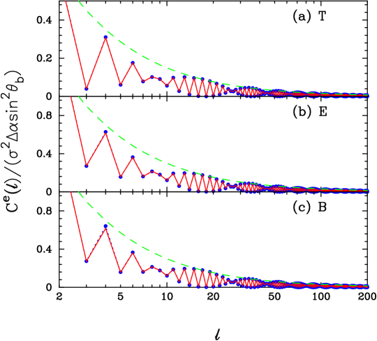
Figure 3: Destriping power spectrum errors for the ring torus geometry analysed in the text. A boresight angle of $85^{\circ}$ has been assumed. The upper panel (a) shows the results for the temperature power spectrum , the central panel (b) shows results for the polarization E-mode power spectrum and the lower panel (c) shows results for the B-mode. In each case, the (blue) points show the results from $10^{4}$ simulations with parameters as discussed in the text. The (red) solid lines show the analytic predictions of equations (30a)- (30c). The (green) dashed lines show the high $\ell$ envelope $\pi/(2\ell+1)$ for $T$ and $2\pi/(2\ell+1)$ for $E$ and $B$.

Some features of these results (useful for understanding real experiments) are worth pointing out. If $\sigma^{2}_{q}=\sigma^{2}_{u}$, the error power spectra of the $E$ and $B$ modes are identical. Furthermore, the dominant terms in both power spectra are the $\hat{G}^{+}_{\ell m}$ terms which are similar to the $\hat{P}_{\ell}^{m}$ terms at high multipoles. Thus, we expect the error power spectra in the $E$ and $B$ modes to have about twice the amplitude of the temperature error power spectrum. The ring variances $\sigma^{2}_{q}$ and $\sigma^{2}_{u}$ are determined largely by the white noise in the TOD and the scanning geometry (equation 6), and so differences in the detector noise levels will directly effect the destriping error contributions to the power spectra. Finally, if $\langle t^{2}_{q_{1}}\rangle=\langle t^{2}_{q_{2}}\rangle$, equation (30d) show that destriping errors on the TE (denoted X in this paper) power spectrum will be identically zero, even if the destriping errors are large.

Figure 3 compares equations (30a)–(30c) with the average power spectra determined from $10^{4}$ simulations as described in Section 3.1 (see Figure 1). (We do not plot $\tilde{C}^{X}_{\ell}$ since the simulations assume identical ring variances for each detector and so the error power spectrum averages to zero. The dashed lines in Figure 3 show the envelopes $\tilde{C}^{e}_{\ell}\propto 1/(2\ell+1)$, valid in the limit $\ell\gg 1$ for a boresight angle $\theta_{b}=\pi/2$ (E04). Evidently, the simulations and theory are in perfect agreement. The ‘sawtooth’ pattern, with a $1/\ell$, envelope is a characteristic feature of map making in a total power experiment with a near ring torus scanning geometry. This pattern can be seen in, for example, the analysis of Planck simulations described by A06. It is worth emphasing the point made in the introduction that destriping errors for a Planck-like experiment cannot be removed by applying an ‘optimal’ least-squares map making code, since it is not possible to remove the ‘irreducible’ striping errors fixed by the detector white noise and scanning. Furthermore, if the detector $1/f$ knee frequencies are comparable to, or less than, the spin frequency, simple destriping with a small number of baselines coefficients will be sufficient to get close to the irreducible striping errors (see e.g. E05, KKP05, A06). The analysis presented in this Section shows that for a Planck-like experiment, the effects of residual striping errors in the $T$, $E$ and $B$ power spectra will be ‘pinned’ to the detector white noise level (since this largely fixes the variance of the baseline offsets) and will always dominate over the white noise level at low multipoles.

3.3 Pixel noise covariances

Optimal power spectrum estimators based on maps require the pixel-pixel noise covariance matrices. In the hybrid power spectrum approach discussed in E04 and E06, PCL estimators are applied at high multipoles and quadratic maximum likelihood (QML) estimators (e.g. Tegmark 1997c; Tegmark and de Oliveira-Costa 2001) are applied on degraded resolution maps to determine the power spectra at low multipoles. In the examples discussed in E04 and E06, noise was either ignored for the QML estimates, or assumed to be uncorrelated. The results of the previous Section show that in a realistic Planck-like experiment, destriping errors will dominate over white noise at low multipoles and hence must be quantified to obtain accurate estimates of the power spectra and their statistical distributions. The same is true for any map-based power spectrum estimator, including map-based Gibbs sampling methods (see e.g. Larson et al. 2006).

For a Planck-size map, containing typically $\sim 2\times 10^{7}$ pixels it is not feasible either to compute or store a full pixel-pixel covariance matrix. However, since destriping errors are important only at low multipoles, all that is required for power spectrum estimation is an accurate model for the pixel-pixel covariance matrices in low resolution maps. In fact, for the ring torus geometery described in the previous Section, it is possible to calculate these covariance matrices analytically.

The power spectra computed in the previous Section are, of course, invariant with respect to the orientation of the spherical coordinate system, whereas the Stokes parameters $Q$ and $U$ and their associated pixel covariance matrices are not. In the ring torus scanning geometry, the spin axis defines a fixed plane in the sky (the ecliptic plane for a Planck-type experiment). A common choise is to pick the $z$-axis of the spherical coordinate system to be perpendicular to this plane. We therefore rotate the maps from the coordinate system shown in Figure 2 to a new coordinate systems where the empty holes in the maps lie at the ‘ecliptic’ poles.

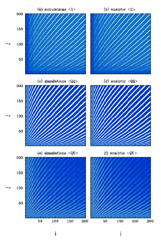
Figure 4: Pixel-pixel covariance matrices for reduced resolution ($\Delta\theta_{c}=10^{\circ}$ pixels) maps for a ring torus geometry with a boresight angle $\theta_{b}=85^{\circ}$. Since the covariance matrices are four-fold symmetric, we show just the lower quadrant of $202\times 202$ elements. The figures to the left show the results of $10^{4}$ simulations (the same set of simulations used to construct the power spectra shown in Figure 3) for the $II$ covariance (panel (a)), $QQ$ covariance (panel (b)) and $QU$ cross-covariance (panel (c)). (The $UU$ covariance looks identical to the $QQ$ covariance.) The figures to the right show the analytic expressions of equations (33a)– (3.3).

We assume that the low resolution maps are constructed by first convolving the high resolution maps with a Gaussian of width $\theta_{s}$ and repixelising to lower resolution. This is equivalent to multiplying the rotated harmonic coefficients (17a)– (17c) by

$$f_{\ell}={\rm exp}\left(-{1\over 2}\ell(\ell+1)\theta_{s}^{2}\right),$$ (31)

and synthesising new maps. Define the auxilliary functions

$$\hat{\Phi}_{\ell m} = \sum_{m^{\prime}}\hat{P}_{\ell m^{\prime}}(\cos\theta_{b})d^{\ell}_{m^{\prime}m}(\pi/2)I(m^{\prime}),$$ (32a)

$$\hat{\Gamma}^{+}_{\ell m} = \sum_{m^{\prime}}\hat{G}^{+}_{\ell m^{\prime}}(\cos\theta_{b})d^{\ell}_{m^{\prime}m}(\pi/2)I(m^{\prime}),$$ (32b)

$$\hat{\Gamma}^{-}_{\ell m} = \sum_{m^{\prime}}\hat{G}^{-}_{\ell m^{\prime}}(\cos\theta_{b})d^{\ell}_{m^{\prime}m}(\pi/2)I(m^{\prime}).$$ (32c)

After some algebra, we can compute the pixel-pixel covariance matrices of the synthesised maps:

$$\langle I_{i}I_{j}\rangle = {\pi\over 2}\sigma^{2}\sin^{2}\theta_{b}\Delta\alpha\sum_{\ell_{1}\ell_{2}}\sum_{m}\hat{P}_{\ell_{1}m}(\cos\theta_{i})\hat{P}_{\ell_{2}m}(\cos\theta_{j})\hat{\Phi}_{\ell_{1}m}\hat{\Phi}_{\ell_{2}-m}f_{\ell_{1}}f_{\ell_{2}}\cos(m(\phi_{i}-\phi_{j})),$$ (33a)

$$\langle Q_{i}Q_{j}\rangle = {\pi\over 16}\sigma^{2}\sin^{2}\theta_{b}\Delta\alpha\sum_{\ell_{1}\ell_{2}}\sum_{m}\big{[}\left(\hat{\Gamma}^{+}_{\ell_{1}m}\hat{\Gamma}^{+}_{\ell_{2}-m}-\hat{\Gamma}^{-}_{\ell_{1}m}\hat{\Gamma}^{-}_{\ell_{2}-m}\right)\left(\hat{G}^{+}_{\ell_{1}m}(i)\hat{G}^{+}_{\ell_{2}-m}(j)-\hat{G}^{-}_{\ell_{1}m}(i)\hat{G}^{-}_{\ell_{2}-m}(j)\right)+$$

$$\qquad\qquad\left(\hat{\Gamma}^{-}_{\ell_{1}m}\hat{\Gamma}^{+}_{\ell_{2}-m}-\hat{\Gamma}^{+}_{\ell_{1}m}\hat{\Gamma}^{-}_{\ell_{2}-m}\right)\left(\hat{G}^{-}_{\ell_{1}m}(i)\hat{G}^{+}_{\ell_{2}-m}(j)-\hat{G}^{+}_{\ell_{1}m}(i)\hat{G}^{-}_{\ell_{2}-m}(j)\right)\big{]}f_{\ell_{1}}f_{\ell_{2}}\cos(m(\phi_{i}-\phi_{j})),$$

$$\langle Q_{i}U_{j}\rangle = {\pi\over 16}\sigma^{2}\sin^{2}\theta_{b}\Delta\alpha\sum_{\ell_{1}\ell_{2}}\sum_{m}\big{[}-\left(\hat{\Gamma}^{+}_{\ell_{1}m}\hat{\Gamma}^{+}_{\ell_{2}-m}-\hat{\Gamma}^{-}_{\ell_{1}m}\hat{\Gamma}^{-}_{\ell_{2}-m}\right)\left(\hat{G}^{+}_{\ell_{1}m}(i)\hat{G}^{-}_{\ell_{2}-m}(j)-\hat{G}^{-}_{\ell_{1}m}(i)\hat{G}^{+}_{\ell_{2}-m}(j)\right)+$$

$$\qquad\qquad\left(\hat{\Gamma}^{+}_{\ell_{1}m}\hat{\Gamma}^{-}_{\ell_{2}-m}-\hat{\Gamma}^{-}_{\ell_{1}m}\hat{\Gamma}^{+}_{\ell_{2}-m}\right)\left(\hat{G}^{+}_{\ell_{1}m}(i)\hat{G}^{+}_{\ell_{2}-m}(j)-\hat{G}^{-}_{\ell_{1}m}(i)\hat{G}^{-}_{\ell_{2}-m}(j)\right)\big{]}f_{\ell_{1}}f_{\ell_{2}}\sin(m(\phi_{i}-\phi_{j})),$$

where $\theta_{i}$, $\phi_{i}$ are the angular coordinates of pixel $i$. For simplicity, we have assumed that $\sigma^{2}_{q}=\sigma^{2}_{u}=\sigma^{2}$, thus $\langle U_{i}U_{j}\rangle=\langle Q_{i}Q_{j}\rangle$.

Figure 4 compares the analytic expressions of equations (33a) -(3.3) with the results of numerical simulations. The simulation results are based on the same set of simulations used to generate Figure 3, but degraded to a pixel size of $\Delta\theta_{c}=10^{\circ}$ after smoothing with a Gaussian of width $\theta_{s}=8.5^{\circ}$. At this resolution a full map consists of only $404$ pixels and because of the four-fold symmetry of the covariance matrices, we plot only the lower quadrant (pixel indices are ordered as $i=j^{\prime}+N_{\phi}^{\prime}(i^{\prime})(i^{\prime}-1)$ where the index $i^{\prime}$ labels the polar angle $\theta$, with $i^{\prime}=1$ corresponding to the ecliptic pole, $j^{\prime}$ labels the azimuthal angle $\phi^{\prime}$ and $N_{\phi}(i^{\prime})$ denotes the number of azimuthal angle bins at polar angle $i^{\prime}$). The analytic results are in perfect agreement with the numerical simulations. The general behaviour of these pixel-pixel covariances is straightforward to understand. The pixel noise is highly correlated along the scanning rings, almost great circles at this resolution, modulated by the hit count distribution. The $\langle QU\rangle$ cross-covariances are considerably smaller than the $\langle QQ\rangle$ and $\langle UU\rangle$ covariances and could almost certainly be ignored for most purposes.

4 More Realistic Simulations

The model described in the previous Section is useful for gaining physical insight into the effects of destriping errors in CMB experiments. However, the focal plane and scanning geometry are highly idealised and the baseline offsets are assumed to be strictly uncorrelated. The model offers, at best, a first approximation to the effects of destriping errors in a realistic Planck-type experiment. In this Section, we discuss a simple, fast, and practical Monte-Carlo method for estimation pixel noise covariances for a more realistic experimental configuration.

The focal plane geometry is modelled by the four Planck $143$ GHz polarization sensitive bolometer pairs (see e.g. Figure 3 of Delabrouille and Kaplan 2002) . This consists of two pairs of bolometers in the $Q$-configuration of Figure 1 and two pairs in the $U$-configuration aligned along the scan direction. We assume a scanning pattern in which the spin axis scans along the ecliptic plane but with a slow precession of $5^{\circ}\sin(2\phi)$. The focal plane and scanning geometry therefore violate (mildly) the assumptions of the ring torus model described in the previous Section.

The input CMB maps are Gaussian realisations of a spatially flat $\Lambda$-dominated CDM universe with the WMAP3 parameters ($\Omega_{b}h^{2}=0.0223$, $\Omega_{m}h^{2}=0.127$, $h=0.73$, $n_{s}=0.95$, $\tau=0.090$, $\sigma_{8}=0.74$, in the notation of Spergel et al. 2006). For these simulations the $B$-mode anistropy is set to zero, i.e. the tensor mode amplitude is assumed to be negligible and the effects of gravitational lensing (see e.g. Lewis and Challinor, 2006, and references therein) are ignored. A Gaussian smoothing with $\theta_{s}=0.425^{\circ}$ was applied and maps were generated with a pixel size of $\Delta\theta_{c}=0.5^{\circ}$. The input power spectra for one such (noise free) realisation are shown in Figure 5 and the $I$, $Q$ and $U$ maps for this realisation are shown in the left hand panels of Figure 7. TOD were generated for each of the eight bolometers in $1080$ scanning rings consisting of $1080$ ring pixels. The scanning rings partially overlap with a width of $30^{\prime}$ and a separation of $20^{\prime}$. Only Gaussian white noise was included in the TOD (with an rms of $54\mu$K per ring pixel) so the simulations are designed to compute the irreducible white noise contribution to the destriping errors discussed in Section 2. Destriping was performed by determining one baseline coefficient for each detector scanning ring. This is done by minimising for each detector

$$\tilde{\chi}^{2}=\sum_{p}\sum_{ijkk^{\prime}\subset p}{1\over 2\sigma^{2}n_{p}}(y^{ik}-a_{k}-\hat{q_{i}}-y^{jk^{\prime}}+a_{k^{\prime}}+\hat{q_{j}})^{2}+\lambda\left(\sum_{k}a_{k}\right)^{2}$$ (34)

where $n_{p}$ is the hit count in map pixel $p$ and $k$ denotes the scanning ring. The second term enforces the condition $\sum a_{k}=0$. Provided $\lambda$ is chosen to be large enough, the solutions for the $a_{k}$ (and their errors) are independent of $\lambda$. The correction terms $\hat{q}_{i}$ and $\hat{q}_{j}$ in (34) correct for the small orientation dependent polarization contribution to the TOD (equation 8) determined from the $Q$ and $U$ maps constructed from all of the detectors. (Maps from the destriped noisy TODs were constructed by a straightforward generalisation of equations (15a)– (15c) to eight detectors.) The solution for the offsets $a_{k}$ is therefore iterative: offsets are determined by first minimising (34) with $\hat{q_{i}}$ set to zero, constructing $I$, $Q$ and $U$ maps using these offsets and then recomputing offsets by using the $Q$ and $U$ maps to compute the polarization corrections $\hat{q}_{i}$. The solutions converge very rapidly to a stable solution. The first term in the $\chi^{2}$ of equation (34) is an approximation to

$$\chi^{2}=({\bf y}-{\bf F}{\bf a})^{T}{\bf Z}^{T}{\bf C}_{n}^{-1}{\bf Z}({\bf y}-{\bf F}{\bf a}),$$ (35)

derived by substituting the solution (5a) back into equation (4).

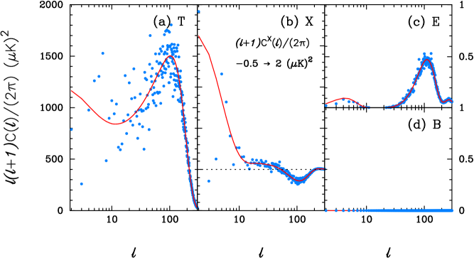
Figure 5: The (blue) points show $T$, $X$, $E$ and $B$ power spectra of a single Gaussian realisation of a $\Lambda$CDM model with WMAP3 parameters (see text) at a resolution of $\theta_{\rm FWHM}=1^{\circ}$. The tensor amplitude in this model is set to zero. The (red) lines show the expectation values of the power spectra for this $\Lambda$CDM model. The input $I$, $Q$ and $U$ maps for this realisation are shown in the left hand panels of Figure 7.

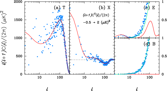
Figure 6: The (blue) points show CMB power spectrum of a noisy realisation of the $\Lambda$CDM model shown in Figure 5, but after polarization destriping as described in the text. The noise parameters, focal plane geometry and scanning strategy have been chosen to match the Planck $143$ GHz polarization sensitive bolometers, but with the noise renormalised to compensate for the degraded resolution of the simulations. The (red) lines show the expectation values of the power spectra for this $\Lambda$CDM model as plotted in Figure 5. The (green) lines in panels (c) and (d) show the white noise errors on the polarisation power spectra.

The white noise level applied to the TOD was chosen so that the final maps have a white noise amplitude in each $30^{\prime}\times 30^{\prime}$ map pixel about equal to that expected for the $8$ polarized Planck $143$GHz detectors. The simulations should thus give a good indication of what we might expect from Planck at low multipoles. The resolution of the simulation (set by $1080$ scanning rings, compared to the $8640$ scanning rings for Planck) has been chosen so that it is possible to generate large numbers of simulations of the TODs on a workstation rather than a supercomputer. It is straightforward to generalise the simulations described in this Section to full Planck resolution and to relax the assumptions of white noise in the TOD and one baseline per detector ring.

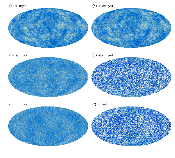
Figure 7: The pictures to the left (a)-(c) show the noise free input $I$, $Q$ and $U$ maps used to generate the power spectra plotted in Figure 5. The pictures to the right (d)-(f) show the output maps with realistic instrument noise and polarization destriping corresponding to the power spectra plotted in Figure 6. Note that the $Q$ and $U$ maps are dominated by white noise, though some signal from low multipoles can be discerned.

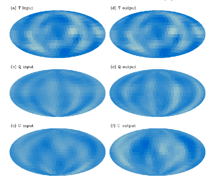
Figure 8: The maps from Figure 7 smoothed with a Gaussian beam of FWHM $20^{\circ}$ and pixelised into maps with $10^{\circ}\times 10^{\circ}$ pixels. The Planck-like polarization maps (e) and (f) are dominated by signal at low multipoles (see Figures 6c and 6d), but noise from residual striping errors is also visible at this resolution.

Figure 6 shows the power spectra for the realisation of Figure 5 but now including destriping and white noise as described above. The maps corresponding to these power spectra are shown in the right hand panels of Figure 7. The white noise level for these simulations is so low that it cannot be seen in the $T$ and $X$ power spectra. However, the $E$ and $B$ mode power spectra are dominated by white noise at $\ell\lower 2.15277pt\hbox{$\;\buildrel>\over{\sim}\;$}20$. The $E$ mode power spectrum is signal dominated at $\ell\lower 2.15277pt\hbox{$\;\buildrel<\over{\sim}\;$}10$ and at these low multipoles the dominant source of noise comes from destriping errors. Since the white noise for each detector is assumed to be the same, the noise contributions to the $E$ and $B$ power spectra are almost identical. Comparing the right hand panels of Figure 7 with the input maps, one can see that the $Q$ and $U$ maps are dominated by white noise, but some large-scale CMB features can be discerned in these noisy maps.

Figure 8 shows the maps of Figure 7 smoothed with a Gaussian of width $\theta_{s}=8.5^{\circ}$ and repixelised onto pixels of width $\Delta\theta_{c}=10^{\circ}$. The large scale CMB features in the output $Q$ and $U$ maps are now clearly visible and the dominant source of errors are stripes aligned (almost) along great circles in the sky. If Planck works as expected (i.e. no unexpected and ‘uncorrectable’ sources of low frequency noise) the polarization maps at this frequency should be signal dominated on large scales.

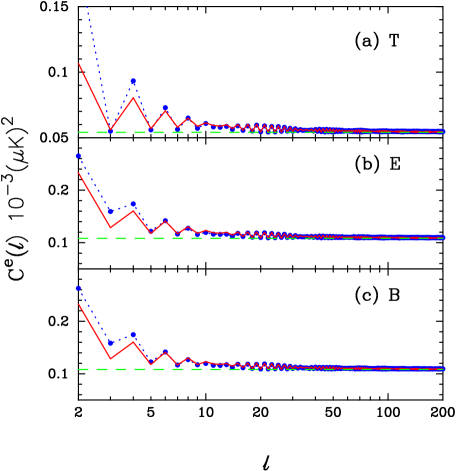
Figure 9: The (blue) circles show the mean error power spectra for $4000$ simulations of the type shown in right hand panels of Figure 7.The (green) dashed line shows the white noise level to which these power spectra converge at high multipoles. The (red) solid lines shows sum of the white noise levels and the analytic predictions of equations (30a)- (30c) for a ring-torus geometry with boresight angle $86.15^{\circ}$.

Figure 9 shows the error power spectra determined from $4000$ simulations with parameters as described above (plotted as the blue circles). The (green) dashed lines in the Figure show the white noise level expected for each power spectrum. The (red) lines show the ring-torus model of equations (30a) - (30c) scaled to provide a good fit to the numerical results. (A boresight angle of $86.15^{\circ}$, appropriate for the polarized $143$GHz Planck detectors, has been used for these predictions.) The ring-torus model deviates slightly from the numerical results at $\ell\lower 2.15277pt\hbox{$\;\buildrel<\over{\sim}\;$}5$, but provides a highly accurate match to the error power spectra at higher multipoles. It is therefore feasible to use the error model to fit and subtract the noise biases to the power spectrum estimates for the $E$ and $B$ modes at $\ell\lower 2.15277pt\hbox{$\;\buildrel>\over{\sim}\;$}5$. It is also worth pointing out that the error power spectra will increase the variances of the power spectrum estimates approximately as

$$\langle(\Delta C_{\ell})^{2}\rangle\approx{2\over(2\ell+1)}(C^{\rm CMB}_{\ell}+C^{e}_{\ell})^{2},$$ (36)

and will introduce coupling between coefficient of different $\ell$ (see below).

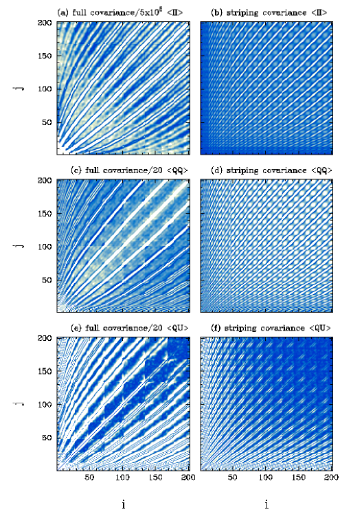
Figure 10: The panels to the left show one quadrant of the full pixel-pixel noise covariance matrices (i.e. signal+destriping errors+white noise) estimated from $4000$ simulations of degraded resolution destriped maps such as those shown in Figures 8d – 8f. The panels to the right show the contribution to these covariance matrices arising from destriping errors alone. These can be compared to the ring-torus model plotted in Figure 4. Note that the full covariance matrices have been divided by scaling factors to render them visible: the $\langle II\rangle$ covariance plotted in (a) has been divided by a factor of $5\times 10^{5}$; the $\langle QQ\rangle$ and $\langle QU\rangle$ covariances in (c) and (e) have each been divided by a factor of $20$.

Pixel-pixel covariance matrices averaged over $4000$ degraded resolution maps, such as those plotted in Figure 4, are shown in Figure 10. The left hand panels show the full pixel-pixel covariance matrices, which include signal, destriping errors and white noise. The panels to the right show the contribution to the pixel noise arising from destriping errors alone. These can be compared to the equivalent figures for the ring torus geometry shown in Figure 4. Apart from differences in the amplitudes arising from differences between the dispersion of the ring offsets, the additional structure seen in Figure 10 is caused by the slow precession in the scanning strategy.

The left hand panel of Figure 11 shows the coviariance matrix for the ring offsets $\langle a_{i}a_{j}\rangle$ for one detector determined by averaging over $4000$ simulations. The ring offset covariance matrices are dominantly diagonal, as assumed in the ring torus model of Section 3, but there are some low amplitude correlations particularly with the rings separated by $\Delta\phi\approx\pi$ in ecliptic longtitude. The panel to the right shows the covariance matrix given by the inverse of the Fisher matrix computed from the $\tilde{\chi}^{2}$ of equation (34):

$$\left.\begin{array}[]{ccc}F_{kk}=&{\partial^{2}\tilde{\chi}^{2}\over\partial a_{k}^{2}}=&\sum_{p}\sum_{ik\subset p}{1\over\sigma^{2}n_{p}}+2\lambda,\\ F_{kk^{\prime}}=&{\partial^{2}\tilde{\chi}^{2}\over\partial a_{k}\partial a_{k}^{\prime}}=&\sum_{p}\sum_{ijkk^{\prime}\subset p}{-1\over\sigma^{2}n_{p}}+2\lambda,\end{array}\right\}$$ (37)

which depends only on the scanning pattern and the TOD variance $\sigma^{2}$. The theoretical covariance matrix (37) provides an excellent match to the empirical covariance matrix derived from destriping.

Using $1/8$th of the number of rings for Planck it is feasible, as shown in this Section, to analyse noise power-spectra and estimate the pixel-pixel noise covariance matrices of low resolution maps by brute force simulations of the TOD. At full Planck resolution this will become computationally challenging, if not impossible. For example, suppose we wish to analyse low resolution Planck maps consisting of $10^{4}$ pixels, one would probably require more than $10^{5}$ simulations of the TOD at each frequency to accurately characterise the pixel noise covariance matrices. However, Figure 11 suggests that full simulations of the TOD are not required. Instead, we can decompose the noise into an ‘uncorrelated’ component described by the $3\times 3$ matrices of equation (13) and a correlated component quantifying the destriping errors given by the Fisher matrix of (37). We will focus on modelling the destriping errors in the remainder of this Section.

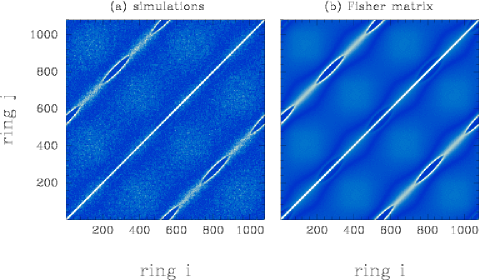
Figure 11: Figure 11a shows the covariance matrix of the destriped ring offsets for a single bolometer determined from 4000 simulations. Figure 11b shows the theoretical covariance matrix computed from equation (37).

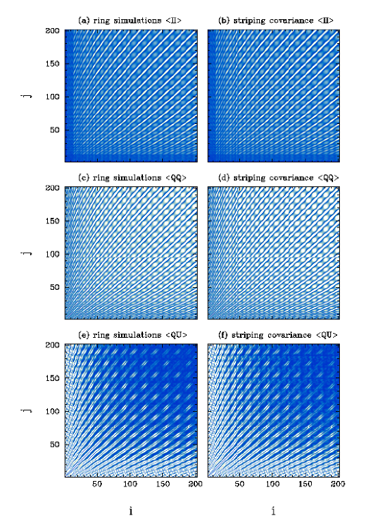
Figure 12: The right hand panels are identical to the right hand panels of Figure 11 and show the pixel-pixel covariance matrices arising from destriping errors alone. The left hand panels show the pixel covariance matrices from $10,000$ simulations generated from Gaussian realisations of ring offsets with the theoretical covariance matrices of equation (37).

Given the Fisher matrix (37) it is straightforward, and very fast, to generate simulations of correlated baseline coefficients and to compute $I$, $Q$ and $U$ maps and error power spectra. These maps can then be degraded to a lower resolution after smoothing by a Gaussian (31) or a more complex function (for example, if one wants to minimise contamination from the Galaxy). An example is shown in Figure 12. In this Figure, the left hand panels are identical to the right hand panels of Figure 10 show the destriping contributions to the pixel covariances derived from full simulations of the TOD. The panels to the right show the destriping covariances from ring simulations assuming that the ring coefficients are Gaussian distributed with a covariance matrix $F_{kk^{\prime}}^{-1}$. The results are essentially identical to those from the simulations of the TODs.

Monte-Carlo simulations of the baseline offsets is therefore provide an entirely feasible approach to analysing the complex striping noise for Planck. The map comparisons in A06 show that for realistic ‘$1/f$’ detector noise it is possible to get close to the ‘irreducible’ destriping errors using a small number of baseline offsets (as mentioned in the introduction, one offset per ring comes close to the ‘optimal’ map solution) and so a manageable number of baseline offsets can be used in the Monte-Carlo simulations. The example shown in Figure 6 shows that the $E$-mode power spectrum for the $143$GHz Planck channel should be signal dominated at multipoles $\ell\lower 2.15277pt\hbox{$\;\buildrel<\over{\sim}\;$}10$ and at $\ell\lower 2.15277pt\hbox{$\;\buildrel<\over{\sim}\;$}20$ destriping errors will be the dominant source of noise. It is therefore important to model the destriping noise from Planck. The amplitude of $B$-mode spectrum is unknown (for a recent review see Efstathiou and Chongchitnan, 2006) and may well be lower than the Planck detection threshold, corresponding to a tensor-scalar ratio $r\sim 0.1$ (SPP05) An accurate analysis of destriping errors will therefore be essential for the analysis of primordial $B$-mode anistropies (particularly for the possible detection of a ‘reionisation bump’ at $\ell\lower 2.15277pt\hbox{$\;\buildrel<\over{\sim}\;$}$, which cannot be observed in ground based experiments).

Finally, we mention that if the CMB fluctuations are an isotropic Gaussian random field, then we expect the harmonic coefficients to satistfy

$$\langle a_{\ell m}a^{*}_{\ell m^{\prime}}\rangle=C_{\ell}\delta_{\ell\ell^{\prime}}\delta_{mm^{\prime}}.$$ (38)

The simulations described above show that the destriping errors are well approximated by a Gaussian random field and, of course, Gaussianity is assumed in generating simulations from the covariance matrices of the ring offsets. However, the striping errors, although Gaussian, are evidently anisotropic since they are highly correlated along the scan direction. Failure to model the destriping errors could therefore have a significant effect on tests for non-Gaussianity in the Planck data. The striping errors will also introduce correlations in the harmonic coefficients. For example, for the temperature anisotropies, E05 used the ring torus model to show that the striping errors lead to correlations:

$$\langle a^{e}_{\ell m}a^{*e}_{\ell^{\prime}m^{\prime}}\rangle={\pi\over 4}\sigma^{2}\sin^{2}\theta_{b}\Delta\alpha\delta_{mm^{\prime}}\sum_{m_{1}m_{2}}\hat{P}_{\ell m_{1}}\hat{P}_{\ell^{\prime}m_{2}}I(m_{1})I(m_{2})d^{\ell}_{m_{1}m}d^{\ell^{\prime}}_{m2m^{\prime}}(\pi/2),$$ (39)

violating the statistical isotropy of equation (38). The ring torus model of Section 3 can be used to show that destriping errors introduce similar correlations in the polarization harmonic coefficients. In assessing non-Gaussianity, using either map based statistics or statistics based on harmonic coefficients, it will be important to model the effects of destriping errors. This can be done at full Planck resolution by generating large numbers of simulations using ring covariance matrices, rather than simulations of the TODs.

5 Conclusions

This paper has presented an analysis of destriping errors in temperature and polarization maps for a Planck-like experiment, generalising the results of E05 to polarization. For a simple detector geometry and ring torus scanning pattern, we have shown that it is possible to compute analytically the effects of striping errors on both the power spectra and pixel-pixel covariances.

In Section 4 we have compared the ring torus model against simulations adopting the focal plane geometry of the Planck polarized $143$GHz detectors and a slowly precessing scan strategy. The ring torus model provides a very accurate description of the noise power spectra at $\ell\lower 2.15277pt\hbox{$\;\buildrel>\over{\sim}\;$}5$. The white noise in the detector TODs in the numerical simulations was chosen to match the expected noise levels of the Planck detectors in $30^{\prime}\times 30^{\prime}$ pixels. Thus at low multipoles, the simulations should give a good indication of the expected performance of Planck. The simulations show that Planck polarization maps should be signal dominated at large scales. The $E$-mode power spectrum should be signal dominated at $\ell\lower 2.15277pt\hbox{$\;\buildrel<\over{\sim}\;$}10$ and destriping errors will be the dominant source of noise in the $E$- and $B$-mode power spectra at $\ell\lower 2.15277pt\hbox{$\;\buildrel<\over{\sim}\;$}20$. Destriping errors will therefore need to be modelled accurately in the analysis of the polarization power spectra from Planck.

As discussed in E06, since the noise is expected to be white at high multipoles, near-optimal estimates of the power spectra and their covariances can be obstained using a hybrid power spectrum estimator. Provided one has a model for the pixel covariance matrices, the low multipoles can be determined by applying a maximum likelihood estimator to low resolution maps. Section 4 shows that a model for the pixel covariances for maps of arbitrary resolution can be constructed accurately using fast simulations based on the statistical properties of the destriping baseline offsets, rather than simulations of the full TOD. Such fast simulations will be useful for other purposes, for example, in assessing the signficance of tests for non-Gaussianity in the Planck maps.

Acknowledgements: I thank members of the Cambridge Planck Analysis Centre, especially Anthony Challinor and Mark Ashdown, for helpful discussions.

References

- [Ash2006] Ashdown M.A.J., et al., 2006, submitted to A&A. astro-ph/0606348.
- [BFJS2001] Borrill J., Ferreira P. G., Jaffe A. H., Stompor R., 2001, In ‘Mining the Sky’, Proceedings of the MPA/ESO/MPE Workshop, Edited by A. J. Banday, S. Zaroubi, and M.Bartelmann. Springer-Verlag, Heidelberg, p403.
- [BS931993] Brink D.M., Satchler G.R,. 1993, Angular Momentum, third edition, Oxford University Press, Oxford.
- [BMMDMBM971997] Burigana C., Malaspina M., Mandolesi N., Danese L., Maino D., Bersanelli M., Maltoni M., 1997, Internal Report ITESRE. astro-ph/9906360.
- [CC052005] Challinor A.D., Chon G., 2005, MNRAS, 360, 509.
- [D981998] Delabrouille, J., 1998, A&A Suppl. Ser., 127, 555.
- [DK012002] Delabrouille, J., Kaplan J., 2002, Proceedings of the Pol2001 Astrophysical Polarised Backgrounds’ conference, Bologna, AIP Conference Proceedings, 609, 135.
- [DKP012001] Doré O., Teyssier R., Bouchet F.R., Vibert D., Prunet S., 2001, A&A, 374, 358.
- [E042004] Efstathiou G., 2004, MNRAS, 439, 603.
- [E052005] Efstathiou G., 2005, MNRAS, 356, 1549.
- [E062006] Efstathiou G., 2006, MNRAS, 370, 343.
- [E062006] Efstathiou G., Chongchitnan S. 2006, Prog. Theor. Phys. Suppl., 163, 204.
- [Hetal22002] Hivon E., Górski K.M., Netterfield C.B., Crill B.P., Prunet S., Hansen F., 2002, ApJ, 567, 2.
- [KKS1997] Kamionkowski M., Kosowsky A., Stebbins A., 1997, PRD, 55, 7368.
- [KKPMB032003] Keihänen E., Kurki-Suonio H., Poutanen T., Maino, D., Burigana C., 2004, A&A, 438, 287.
- [KKP052005] Keihänen E., Kurki-Suonio H., Poutanen T., 2005, MNRAS, 360, 390.
- [Letal062006] Larson D.L., Eriksen H.K., Wandelt B.D., Górski K.M., Huey G., Jewell J.B., O’Dywer I.J., 2006, ApJ, in press. astro-ph/0608007.
- [LC062006] Lewis A., Challinor, A., 2006, Phys. Rep., 429, 1.
- [Metal991999] Maino D., et al., 1999, A&A Suppl. Ser., 140, 383.
- [NdeGGV011997] Natoli P., de Gasperis G., Gheller C., Vittorio N., 2001, A&A, 372, 346.
- [PO52005] The Planck Consortia, 2005, ‘The Scientific Programme of Planck’, ESA-SCI(2005)1, European Space Agency. astro-ph/0604069. (SPP05)
- [RKACDK002000] Revenu B., Kim A., Ansari R., Couchot F., Delabrouille J., Kaplan J., 2000, A&A Suppl. Ser., 142, 499.
- [SS042004] Slosar A., Seljak, U., 2004, PRD, 70, 3002.
- [Setal062006] Spergel D., et al., 2006, submitted to ApJ. astro-ph/0603449.
- [T97a1997] Tegmark M., 1997a, ApJL, 480, L87.
- [T97b1997] Tegmark M., 1997b, PRD, 56, 4514.
- [T97c1997] Tegmark M., 1997c, PRD, 55, 5895.
- [TdO972001] Tegmark M., de Oliveira-Costa A., 2001, PRD, 64, 063001.
- [VMK881988] Varshalovich, D.A., Moskalev A.N., Khersonskii V.K., 1988, Quantum Theory of Angular Momentum, World Scientific, Singapore.
- [WHB961996] Wright E.L., Hinshaw G., Bennett C.L., 1996, ApJ, 458, L53.