Robust quantitative measures of cluster X-ray morphology, and comparisons between cluster characteristics

Abstract

Aims. To investigate the possible relationships between dynamical status and other important characteristics of galaxy clusters, we conducted a study of X-ray cluster morphology using a sample of 101 clusters at redshift z$\sim$0.05-1 taken from the Chandra archive.

Methods. The X-ray morphology is quantitatively characterized by a series of objectively measured simple statistics of the X-ray surface brightness distribution, which are designed to be robust against variations of image quality caused by various exposure times and various cluster redshifts. Using these measures, we quantitatively investigated the relationships between the cluster X-ray morphology and various other cluster characteristics.

Results. We found: (1) Our measures are robust against various image quality effects introduced by exposure time difference, and various cluster redshifts. (2) The distorted and non-distorted clusters occupy well-defined loci in the L-T plane, demonstrating the measurements of the global luminosity and temperature for distorted clusters should be interpreted with caution, or alternatively, a rigorous morphological characterization is necessary when we use a sample of clusters with heterogeneous morphological characteristics to investigate the L-T or other related scaling relations. (3) Ellipticity and Off-center show no evolutionary effects between high and low redshift cluster subsets, while there may be a hint of weak evolutions for the Concentration and Asymmetry, in such a way that high-z clusters show more distorted morphology. (4) No correlation is found between X-ray morphology and X-ray luminosity or X-ray morphology and X-ray temperature of clusters, implying that interaction of clusters may not enhance or decrease the luminosity or temperature of clusters for extended period of time. (5) Clusters are scattered and occupying various places in the plane composed of two X-ray morphological measures, showing a wide variety of characteristics. (6) Relatively strong correlations in Asymmetry-Concentration and Offcenter-Concentration plots indicate that low concentration clusters generally show high degree of asymmetry or skewness, illustrating the fact that there are not many highly-extended smooth symmetric clusters. Similarly, a correlation between Asymmetry and Ellipticity may imply that there are not many highly-elongated but otherwise smooth symmetric clusters.

1 Introduction

Over the past decade, studies have provided evidence that a significant fraction of galaxy clusters have undergone recent mergers (e.g. Geller & Beers 1982; Dressler & Shectman 1988). These mergers are observed as disturbed cluster morphologies. The important connection between the morphologies of galaxy clusters and cosmological parameters has received much recent attention (Richstone, Loeb, & Turner 1992; Evrard et al. 1993; Mohr et al. 1995). This connection has generally been formulated in terms of the frequency of ‘substructure’ in clusters and from qualitative measures of the frequency of substructure in clusters, investigators have attempted to determine $\Omega_{m}$ (e.g. Richstone et al. 1992) and the power spectrum of primordial density fluctuations (e.g. David et al. 1993) by comparison to Press & Schechter (1974) type predictions of the distribution of collapsed objects.

Methods to quantify structures at optical wavelengths have mostly used both the distribution of cluster galaxies, and lensing. However, the distribution study requires a large number of galaxies, and is more susceptible to contamination from foreground and background objects. Lensing is also sensitive to this contamination, and does not have good spatial resolution except for the central region of a cluster. An alternative method comes from X-ray wavelengths, because cluster mergers compress and heat the intracluster gas, and this can be measured as distortions of the spatial distribution of X-ray surface brightness and temperature. Moreover, X-ray emissivity is proportional to the square of the electron density, and therefore less affected by the superposed structures than optical data. Jones & Forman (1999) visually examined 208 clusters observed with Einstein X-ray satellite and separated these clusters into six morphological classes. They found that about 40% of their clusters displayed some type of ‘substructure’.

However, a more quantitative measure of cluster structure at X-ray wavelengths is desirable to quantitatively test various scenarios related to clusters, including cosmology. Using $Einstein$ images, Mohr et al. (1995) measured emission-weighted centroid variation, axial ratio, orientation, and radial falloff for a sample of 65 clusters, while several other studies used ellipticity (e.g. McMillan et al. 1989; Gomez et al. 1997; Kolokotronis et al. 2001; Melott et al. 2001; Plionis 2002). Buote & Tsai (1995, 1996) used a power ratio method for 59 clusters observed with $ROSAT$, while Schuecker et al. (2001) conducted a study of 470 clusters from $ROSAT$-ESO Flux-Limited X-ray (REFLEX) cluster survey (Böhringer et al. 2000), using sophisticated statistics, such as Fourier elongation test, Lee test, and $\beta$ test.

Despite the success of these studies, all of them are unfortunately limited to clusters in the nearby universe (z $<$ 0.3), where we may expect to see less frequent morphological distortions, and little evolutionary effect. This is due to the fact that, until recently, only a small number of high-z clusters have been known, or observed with sufficient depth and sufficient spatial resolution. With the advent of big-aperture satellites equipped with high spatial-resolution instruments, such as $Chandra$ and $XMM$-$Newton$, together with newly-available lists of distant clusters generated based on various deep cluster surveys, it is finally possible to extend the morphological study to higher redshifts. Indeed, Jeltema et al. (2005) have recently extended the power ratio method of Buote & Tsai to 40 clusters at z=0.15-0.9 using Chandra data, and reported the evolution of cluster morphology between two redshift bins (z$<$0.5 and z$>$0.5).

Extending the morphological study to high redshift is important but a difficult task because of inevitable low data quality associated with high-z clusters. Conventional methods for characterizing the cluster X-ray morphology are often sophisticated and some methods have an advantage of being more directly related to a particular characteristic of a cluster, such as mass, dark matter content, or gravitational potential. However, most of these conventional methods are originally developed to analyze the low redshift clusters with high data quality, and, perhaps because of their intrinsic sophistication, ofter require many photon counts, making the measures rapidly uncertain or unmeasurable as the data quality decreases. Moreover, these methods also often require some interactive processes, and thus, are not suitable for the investigation involving a large dataset with a wide variety of image quality where various systematics should be treated and removed in a consistent manner. Although it is important to try to extend the sophisticated methods to high redshift, a complementary study using the robust measures of the cluster morphology, less sensitive to variation in the data quality and suitable for a large dataset, is much needed, to enable us to study the low-z and high-z universe in a uniform manner.

Here we report our study of X-ray cluster morphology using a sample of 101 clusters at redshift z$\sim$0.05-1 taken from the Chandra archive. The X-ray morphology is quantitatively characterized by a series of objectively-measured simple statistics of X-ray surface brightness, which are designed to be robust against variations of image quality caused by various exposure times and various cluster redshifts. Using these measures, we quantitatively investigated the relationships between the cluster X-ray morphology and various other cluster characteristics.

This paper is organized as follows. In sec 2, we describe our sample and data preparation, while in sec 3, details of our measures are described, and in sec 4, uncertainty and systematics are investigated. Sec. 5 summarizes our results. Throughout the paper, we use $H_{o}$ = 70 km s^-1 Mpc^-1, $\Omega_{m}$=0.3, and $\Omega_{\Lambda}$=0.7, unless otherwise stated.

2 Sample & data preparation

Table 1: The Sample

Name	z	Lbol	Tx	rc	$\beta$	ref
		10${}^{44}erg/s$	keV	kpc
A3562	0.050	3.56	5.2	99	0.472	a
A85	0.052	13.15	6.9	83	0.532	a
HydraA	0.052	6.19	4.3	50	0.573	a
A754	0.053	6.44	9.5	239	0.698	a
A2319	0.056	35.80	11.8	170	0.550	e
A3158	0.059	6.92	5.8	269	0.661	a
A3266	0.059	12.81	8.0	564	0.796	a
A2256	0.060	5.05	6.6	587	0.914	a
A1795	0.063	14.73	7.8	78	0.596	a
A399	0.072	9.75	7.0	450	0.713	a
A2065	0.072	6.72	5.5	690	1.162	a
A401	0.075	16.53	8.0	246	0.613	a
ZwCl1215+0400	0.075	–	–	–	–
A2029	0.077	27.84	9.1	83	0.582	a
A2255	0.080	12.53	6.9	593	0.797	a
A1651	0.083	10.35	6.1	181	0.643	a
A478	0.088	27.49	8.4	98	0.613	a
RXJ1844+4533	0.091	–	–	–	–
A2244	0.102	12.11	7.1	126	0.610	a
RXJ0820.9+0751	0.110	–	–	–	–
A2034	0.110	12.51	7.9	290	0.690	d
A2069	0.115	–	–	–	–
RXJ0819.6+6336	0.119	–	–	–	–
A1068	0.139	7.79	3.6	25	0.520	b
A2409	0.147	–	–	–	–
A2204	0.152	40.57	7.2	67	0.597	a
HerculesA	0.154	–	–	–	–
A750	0.163	–	–	–	–
A2259	0.164	–	–	–	–
RXJ1720.1+2638	0.164	25.58	5.6	–	–	i
A1201	0.169	–	–	–	–
A586	0.171	11.80	7.0	119	0.680	b
A2218	0.171	12.10	7.6	165	0.580	b
A1914	0.171	33.75	10.5	231	0.751	a
A2294	0.178	–	–	–	–
A1689	0.184	36.62	9.2	163	0.690	a
A1204	0.190	–	–	–	–
MS0839.8+2938	0.194	4.51	3.4	40	0.560	b
A1151	0.197	13.50	5.8	16	0.400	b
A520	0.203	22.89	8.59	–	–	j
A963	0.206	12.00	6.8	71	0.500	b
RXJ0439.0+0520	0.208	–	–	–	–
A2111	0.211	9.50	6.9	149	0.490	b
A1423	0.213	–	–	–	–
ZwCl0949+5207	0.214	8.56	4.0	41	0.530	b
MS0735.6+7421	0.216	9.56	4.5	27	0.460	b
A773	0.217	15.60	8.1	190	0.660	b
A2261	0.224	23.90	6.6	62	0.510	b
A1682	0.226	11.00	6.4	384	0.750	b
A1763	0.228	18.40	8.1	168	0.490	b
A2219	0.228	38.90	9.2	189	0.560	b
A267	0.230	12.00	5.5	141	0.620	b
A2390	0.233	40.80	9.2	44	0.460	b
RXJ2129.6+0006	0.235	18.30	5.7	42	0.510	b
RXJ0439.0+0715	0.244	–	–	–	–
A2125	0.247	5.96	3.2	–	–	l
A68	0.255	15.60	6.9	177	0.610	b
ZwCl1454+2233	0.258	18.30	4.4	43	0.590	b
A1835	0.258	48.10	7.4	46	0.550	b
A17582	0.280	23.60	9.0	1149	3.000	h
A697	0.282	30.90	8.2	198	0.580	b
ZwCl1021+0426	0.291	51.30	6.41	–	–	k
A781	0.298	–	–	–	–
A2552	0.299	–	–	–	–
A1722	0.327	11.10	5.8	92	0.510	b
MS1358.4+6245	0.328	9.43	5.5	40	0.460	b
RXJ1158.8+0129	0.352	–	–	–	–
A370	0.357	10.80	6.6	231	0.540	b
RXJ1532.9+3021	0.361	32.90	4.9	47	0.590	b
MS1512.4+3647	0.372	4.10	2.8	42	0.540	b
RXJ0850.2+3603	0.374	–	–	–	–
RXJ0949.8+1708	0.382	–	–	–	–
ZwCl0024+1652	0.390	3.54	4.5	59	0.410	f
RXJ1416+4446	0.400	5.43	3.7	26	0.438	c
RXJ2228.5+2036	0.412	–	–	–	–
MS1621+2640	0.426	10.92	6.8	185	0.563	c
RXJ1347-1145	0.451	116.75	10.3	38	0.571	c
RXJ1701+6412	0.453	6.42	4.5	13	0.396	c
3c295	0.460	14.07	4.3	31	0.553	c

Table 1 (Continued)
 
  Name z Lbol Tx r_c $\beta$ ref 10${}^{44}erg/s$ keV kpc RXJ1641.8+4001 0.464 – – – – CRSSJ0030.5+26 0.500 – – – – RXJ1525+0957 0.516 6.92 5.1 229 0.644 c MS0451-0305 0.540 50.94 8.0 201 0.734 c MS0016+1609 0.541 53.27 10.0 237 0.685 c RXJ1121+2326 0.562 5.45 4.6 427 1.180 c RXJ0848+4456 0.570 1.21 3.2 97 0.620 c MS2053-0449 0.583 5.40 5.5 99 0.610 c RXJ0542-4100 0.634 12.15 7.9 132 0.514 c RXJ1221+4918 0.700 12.95 7.5 263 0.734 c RXJ1113-2615 0.730 4.43 5.6 89 0.639 c RXJ2302+0844 0.734 5.45 6.6 96 0.546 c MS1137+6625 0.782 15.30 6.9 111 0.705 c RXJ1350+6007 0.810 4.41 4.6 106 0.479 c RXJ1716+6708 0.813 13.86 6.8 121 0.635 c MS1054-0321 0.830 28.48 10.2 511 1.375 c RXJ0152-1357³ 0.835 18.40 6.5 – – c WGA1226+3333 0.890 54.63 11.2 123 0.692 c RXJ0910+5422 1.106 2.83 6.6 147 0.843 c RXJ1053.7+5735⁴ 1.134 2.80 3.9 – – g RXJ1252-2927 1.235 5.99 5.2 77 0.525 c RXJ0849+4452 1.260 2.83 5.2 128 0.773 c References: a: Reiprich & Böhringer(2002); b: Ota & Mitsuda(2004); c: Ettori et al(2004); d: Kempner et al(2003); e: O’Hara et al(2004); f: Ota et al. (2004) (R_c & $\beta$ from Ota & Mitsuda(2004); g: Hashimoto et al(2004); h: David & Kempner(2004); i: Mazzota et al. (2001); j: Wu et al. (1999); k: Allen (2000); l: Wang et al. (2004). Comments: (1): Distant southern component A115S is excluded; (2): Distant southern component A1758S is excluded; (3): RXJ0152, both north and south components are treaded as one cluster; (4): RXJ1054, both east and west components are treaded as one cluster.

Almost all clusters are selected from flux-limited X-ray surveys, and data are taken from the Chandra ACIS archive. A lower limit of z = 0.05 or 0.1 is placed on the redshift to ensure that a cluster is observed with sufficient field-of-view with ACIS-I or ACIS-S, respectively. The majority of our sample comes from the $ROSAT$ Brightest Cluster Sample (BCS; Ebeling et al 1998), and the Extended $ROSAT$ Brightest Cluster Sample (EBCS; Ebeling et al. 2000). The BCS sample includes 201 clusters, with the flux limit of 4.4$\times$10^-12 erg s${}^{-1}cm^{-2}$ (0.1-2.4 keV). The authors estimated a sample completeness of 90 % for the 201 BCS clusters, and 75 % for the EBCS clusters. When combined with EBCS, the BCS clusters represent one of the largest and most complete X-ray selected cluster samples, and they are currently the most frequently observed by $Chandra$. As of 2005 October, 55 BCS + 13 EBCS (hereafter BCS) clusters with z $>$ 0.05 (ACIS-I), or z $>$ 0.1 (ACIS-S), are publicly available in the $Chandra$ archive. Additionally we included all clusters from the X-ray flux limited sample of Edge et al. (1990) at z $>$ 0.05 or 0.1 not in the BCS that were observed with the Chandra ACIS. This added 12 more clusters. The Edge et al. sample is estimated to be $\sim$90% complete, and contains the 55 brightest clusters from $EXOSAT$, $HEAO-1$, and $Einstein$.

To extend our sample to higher redshifts, additional high-z clusters are selected from various deep surveys; 10 of these clusters are selected from the $ROSAT$ Deep Cluster Survey (RDCS: Rosati et al. 1998), 10 from the $Einstein$ Extended Medium Sensitivity Survey (EMSS; Gioia et al. 1990; Henry et al. 1992), 14 from the 160 Square Degrees $ROSAT$ Survey (Vikhlinin et al. 1998), 2 from the Wide Angle $ROSAT$ Pointed Survey (WARPS; Perlman et al. 2002), and 1 from the North Ecliptic Pole survey (NEP; Gioia et al 1999), RXJ1054 was discovered by Hasinger et al. (1998), RXJ1347 was discovered in the $ROSAT$ All Sky Survey (Schindler et al. 1995), and 3C295 has been mapped with $Einstein$ (Henry & Henriksen 1986).

The resulting sample we processed contains 120 clusters. At the final stage of our data processing, to employ our full analysis, we further applied a selection based on the total counts of cluster emission, (for details, please see Sec. 4), eliminating clusters with very low signal-to-noise ratio. Clusters whose center is too close to the edge of the CCD are also removed. The resulting final sample contains 101 clusters with redshifts between 0.05 - 1.26 (median z = 0.226), and luminosity between 1.0 $\times$ 10⁴⁴ – 1.2 $\times$ 10⁴⁶ erg/s (median 8.56 $\times$ 10⁴⁴ erg/s) (Fig.1). The final cluster sample together with their published redshifts and bolometric luminosities, if available, as well as $\beta$s and core radii, are listed in Table 1.

We reprocessed the level=1 event file retried from the archive using CIAO v3.1. and CALDB v2.29. For observations taken in the VFAINT mode, we ran the script acis_process_events to flag probable background events, using the information in a 5 $\times$ 5 event island. We also applied the charge transfer inefficiency (CTI) correction and the time dependent gain correction for ACIS-I data, when the temperature of the focal plane at the time of the observation was 153 K. The data were filtered to include only the standard event grades 0,2,3,4,6 and status 0, then multiple pointings were merged, if any. We eliminated time intervals of high background count rate by performing a 3 $\sigma$ clipping of the background level using the script analyze_ltcrv. To prepare the images for analysis, we selected photons in the observed-frame 0.7-8.0 keV and rest-frame 0.7-8 keV bands initially binned into 0.5 ” pixel (see Sec 4 for the binning scheme of later analysis steps). We corrected the images for exposure variations across the field of view, detector response and telescope vignetting.

We detected point sources using the CIAO routine celldetect with signal-to-noise threshold for source detection of three. An elliptical background annulus region was defined around each source such that its outer major and minor axes became three times of the source region. We removed the detected sources, except for a source at the center of the cluster which was mostly the peak of the surface brightness distribution rather than a real point source, and filled the source regions using the CIAO tool dmfilth. The images were then smoothed with Gaussian $\sigma$=5”. We have decided to perform the smoothing, as well as the total-count cut (see sec 4.2.3 for detail) to avoid the case where we have an image predominantly with zero count pixels, which makes the exposure map correction difficult, as well as the determination of the object region (see below), and for the investigation of various systematics (see sec 4). We found that the choice of smoothing-sigma hardly affects our robust morphological values (please see section 4.2.2. for detail).

Some clusters have a chip gap, or bad column inside the extracted cluster region. Most of these clusters, however, were observed with multiple pointings, thus those artifacts were reasonably corrected by exposure map. For those clusters with a single pointing, the artifacts were all crossing the cluster region far (typically more than 2 arcmin) from the cluster center. Using clusters with multiple pointing observations, we discovered that, the effect of these artifacts are negligible on our morphological measures, particularly after the smoothing.

We decided to use isophotal contours to characterize an object region, instead of a conventional circular aperture, because we did not want to introduce any possible bias in the shape of an object. To define constant metric scale to all clusters, we adjusted an extracting threshold in such a way that the square root of detected object area times a constant was 0.5 Mpc, i.e. const$\sqrt{area}$ = 0.5 Mpc. We chose to use the const =1.5, because the isophotal limit of a detected object was best represented by this value.

Figure 1: Distributions of the X-ray bolometric luminosity (Lbol) and redshift (z) for our sample.

3 Morphological measures

3.1 Centroid & second moments

Centroid and centered-second moments are computed using the first and second order moments of the profile:

$$\overline{x}=\frac{\sum\limits_{i\in S}I_{i}x_{i}}{\sum\limits_{i\in S}I_{i}},\;\;\overline{y}=\frac{\sum\limits_{i\in S}I_{i}y_{i}}{\sum\limits_{i\in S}I_{i}}$$ (1)

$$\overline{x^{2}}=\frac{\sum\limits_{i\in S}I_{i}x_{i}^{2}}{\sum\limits_{i\in S}I_{i}}-\overline{x}^{2},\;\;\overline{y^{2}}=\frac{\sum\limits_{i\in S}I_{i}y_{i}^{2}}{\sum\limits_{i\in S}I_{i}}-\overline{y}^{2},\;\;\overline{xy}=\frac{\sum\limits_{i\in S}I_{i}x_{i}y_{i}}{\sum\limits_{i\in S}I_{i}}-\overline{x}\,\overline{y}$$ (2)

where $x_{i}$ and $y_{i}$ are the x-coordinate and y-coordinate of a pixel $i$ of value $I_{i}$ inside area $S$ of an object.

3.2 Ellipticity

Ellipticity is simply defined by the ratio of semi-major (A) and semi-minor axis (B) lengths as:

$$Elli = 1-B/A$$ (3)

where A and B are defined by the maximum and minimum spatial rms of the object profile along any direction and computed by the formula:

$$A^{2} = \frac{\overline{x^{2}}+\overline{y^{2}}}{2}+\sqrt{\left(\frac{\overline{x^{2}}-\overline{y^{2}}}{2}\right)^{2}+\overline{xy}^{2}}$$ (4)

$$B^{2} = \frac{\overline{x^{2}}+\overline{y^{2}}}{2}-\sqrt{\left(\frac{\overline{x^{2}}-\overline{y^{2}}}{2}\right)^{2}+\overline{xy}^{2}}$$ (5)

3.3 Off-center

The degree of off-center is determined by the distance between the centroid and maximum intensity peak:

$$Offcen=\frac{\sqrt{(x_{p}-\overline{x})^{2}+(y_{p}-\overline{y})^{2}}}{3(A+B)}$$ (6)

where, flux peaks in a pixel at x_p, y_p.

3.4 Concentration

The degree of concentration of the surface brightness profile is measured using a method described in Hashimoto et al. (1998), and is defined by the ratio between central 30% and whole 100% elliptical apertures as:

$$Conc = \frac{\sum\limits_{r_{i}<0.3}I(r_{i})}{\sum\limits_{r_{i}<1.0}I(r_{i})}$$ (7)

where, $r_{i}$ is a position of a pixel $i$ in a parameter which scales the ellipse, in unit of A (or B), and computed using the position angle of each pixel ($\theta_{i}$):

$$r^{2}_{i} = [(\frac{cos^{2}\theta_{i}}{A}+\frac{sin^{2}\theta_{i}}{B})(x_{i}-\overline{x})$$ (8)

$$+(\frac{sin\theta_{i}cos\theta_{i}}{A}-\frac{sin\theta_{i}cos\theta_{i}}{B})(y_{i}-\overline{y})]^{2}$$

$$+[(\frac{sin\theta_{i}cos\theta_{i}}{A}-\frac{sin\theta_{i}cos\theta_{i}}{B})(x_{i}-\overline{x})$$

$$+(\frac{sin^{2}\theta_{i}}{A}+\frac{cos^{2}\theta_{i}}{B})(y_{i}-\overline{y})]^{2}$$

3.5 Asymmetry

To measure the degree of asymmetry of the profile around the centroid, an asymmetry index is computed as:

$$Asym=\frac{\frac{1}{2}\sum\limits_{i\in S}|I(x_{i},y_{i})-I(2x_{i}-\overline{x2},2y_{i}-\overline{y2})|}{\sum\limits_{i\in S}I(x_{i},y_{i})}$$ (9)

where,

$$\overline{x2}=\frac{\sum\limits_{i\in S}I_{i}^{2}x_{i}}{\sum\limits_{i\in S}I_{i}^{2}},\;\;\overline{y2}=\frac{\sum\limits_{i\in S}I_{i}^{2}y_{i}}{\sum\limits_{i\in S}I_{i}^{2}}$$ (10)

After testing various centroids, we have chosen to use the second order centroid $\overline{x2}$ and $\overline{y2}$ to make the asymmetry measure less sensitive to the very faint outer structure than the case using simple $\overline{x}$ and $\overline{y}$.

4 Uncertainty and systematics

4.1 Uncertainty

We applied a Monte Carlo simulation to estimate the uncertainties in our measures caused by point sources and Poisson noise. For each cluster image, starting from the image used for real analysis, we added random artificial point sources consistent with $Chandra$ PSF and numbers consistent with the logN-logS given by Campana et al. (2001). We chose to use the real image instead of $\beta$ model, since many of the clusters were not well descried by the $\beta$ model. Poisson noise was then added to the images. We then excised the bright point sources again exactly the same way as the real analysis, followed by smoothing. For each cluster we performed 100 such realizations, and the morphological measures were computed for each realization. We then simply defined our 1 sigma error for each measure to be $rms$ of the distribution of each measure.

4.2 Systematics

4.2.1 Exposure time effect

To investigate the systematic effect of various exposure times on the morphological measures, one of the standard approaches is to simulate lower signal-to-noise data caused by a shorter integration time by scaling the real data by the exposure time, and adding Poisson noise taking each pixel value as the mean for a Poisson distribution. However, this simple rescaling and adding noise process will produce an excessive amount of Poisson noise, because of the intrinsic noise already present in the initial real data. Meanwhile, using a model image with no intrinsic noise, instead of the real data, will not have this problem, however, here we need to approximate the various characteristics of a model to complicated characteristics of a real cluster and this is an almost impossible task, particularly for a dynamically unsettled distorted cluster. To circumvent this problem, we decided to use the real cluster data and employed a series of ‘adaptive scalings’ accompanied by a noise adding process. Namely, to simulate data with integration t=t1, an original unsmoothed image (including the background) taken with original integration time t0 was at first rescaled by a factor R₀/(1-R₀), instead of simple R₀, where R₀=t1/t0, t0$>$t1. That is, an intermediate scaled image I₁ was created from the original unsmoothed image I₀ by:

$$I_{1} = I_{0}\frac{R_{0}}{(1-R_{0})}$$ (11)

Poisson noise was then added to this rescaled image by taking each pixel value as the mean for a Poisson distribution and then randomly selecting a new pixel value from that distribution. This image was then rescaled again by a factor (1-R₀) to produce an image whose signal is scaled by R₀ relative to the original image, but its noise is approximately scaled by $\sqrt{R_{0}}$, assuming the intrinsic noise initially present in the real data is Poissonian. (The derivation of this scaling is described in the Appendix.) Finally, the image was smoothed with Gaussian of $\sigma$=5”.

Figure 2: Simulated exposure time (in ksec) vs various morphological measures for several typical clusters.

Figure 2 shows the effect of exposure time on each morphological measure. For each cluster data, we simulated observations with several shorter exposure times using the method described above, and re-measured our morphological measures for each simulated observation. In Figure 2, we plotted the simulated exposure time (in ksec) against various morphological measures of our sample clusters. For brevity, we only plotted a handful of typical clusters and the data points of the same cluster were connected with a line to illustrate the trend. The figure shows that, for all of our measures, the systematics caused by exposure time are small, demonstrating the relatively robust nature of our measures against the exposure differences. The morphological measures are generally constant over a range of exposure time, except for some clusters at a very short exposure end, where the noise becomes dominant and measures become uncertain.

4.2.2 Redshift effect

To investigate the systematic redshift effect on the morphological measures, we simulated an observation of a cluster at a higher redshift than its actual redshift using the real data, including the effect of waveband shift, a smaller angular size of the object (also equivalent of having a bigger pixel scale and bigger smoothing scale), and dimming of the object signal with respect to the sky. Namely, to simulate an observation at new redshift z=z1, at first, we created an image of restframe 0.7-8 keV band at original redshift z0 of each cluster (z1$>$z0). The image was then corrected for detector response and telescope vignetting. Because the dimming of surface brightness due to the redshift only occurs to the cluster signal, and not to the background, an object-only frame I₀ was created from this restframe image by subtracting a constant background B. However, to approximate the dimming of cluster by the redshift, we cannot simply scale I₀ by $1/(1+z)^{4}$ because the noise will not be correct (we underestimate it). To properly scale I₀ with the proper amount of noise, we employed an adaptive scaling technique similar to the exposure time case in sec 4.2.1. Unlike the exposure time case, however, the intrinsic noise contained in I₀ is not proportional only to I₀ (it is proportional to I₀+B, instead, even if the background B is already subtracted from the signal). This makes the adaptive scaling more complicated, and we need a pixel-to-pixel scaling (or manipulation) rather than just a simple whole-image scaling. Namely, an intermediate scaled image I₁ was created from I₀ by a pixel-to-pixel manipulation:

$$I_{1}(x,y) = \frac{I_{0}(x,y)^{2}R_{1}^{2}}{[I_{0}(x,y)R_{1}+B-R_{1}^{2}(I_{0}(x,y)+B)]}$$ (12)

$$where,$$

$$R_{1} = [(1+z0)/(1+z1)]^{4}$$ (13)

Similarly to the exposure time effect in sec 4.2.1, Poisson noise was then added to I₁. A new dimmed image I₂ whose cluster signal was scaled by R₁ with respect to the original restframe image with proper amount of Poisson noise was then created from this noise-added image I${}_{1}^{{}^{\prime}}$ by a reverse pixel-to-pixel manipulation:

$$I_{2}(x,y) = I_{1}^{{}^{\prime}}(x,y)\frac{I_{0}(x,y)R_{1}+B-R_{1}^{2}[I_{0}(x,y)+B]}{I_{0}(x,y)R_{1}}$$ (14)

Finally, adding back the background B gives,

$$I^{{}^{\prime}}_{2}(x,y) = I_{2}(x,y)+B$$ (15)

This dimmed image I${}^{{}^{\prime}}_{2}$ should be then rebinned by a factor R₂ to account for the angular-size change due to the redshift difference between z0 and z1. However, this simple rebinning again will not correctly reproduce the proper amount of noise caused by the angular-size change due to the redshift effect. To properly adjust, again underestimated noise due to the simple rebinning, the rebinned image was rescaled by a factor 1/(R${}^{2}_{2}$-1), then Poisson noise was added by taking each pixel value as the mean for a Poisson distribution. The final image was created by rescaling back this noise-added image by a factor (R${}^{2}_{2}$-1)/R${}_{2}^{2}$. The factor R${}_{2}^{2}$ in the denominator is necessary to rebin the image in such a way to conserve the surface brightness. (The derivation of these scalings, or manipulations, are described in the Appendix.)

Figure 3: Simulated redshift vs various morphological measures.

Figure 3 shows the effect of redshift on each morphological measure. For one cluster data, we simulated observations with several higher redshifts than its original redshift using the method described above, and re-measured our morphological measures for each simulated observation. In Figure 3, we plotted the simulated redshift (s_redshift) against various morphological measures of our sample clusters. Again, for brevity, we only plotted a handful of typical clusters and the data points of the same cluster were connected with a line to illustrate the trend. The figure shows that, for most of our measures, the systematics caused by redshift are very small. For the concentration index and asymmetry index, there may be a slight trend that high concentration or high asymmetry objects tend to slightly decrease their values as we go to the higher redshifts, thus reducing the contrast between distorted and non-distorted morphologies.

4.2.3 Combining the exposure and redshift effects

Although the exposure time and redshift effects can be treated separately as described in sec 4.2.1. and 4.2.2., these two effects are often coupled, because low redshift clusters are usually observed with shorter exposures than high redshift clusters. Under these conditions, it is often much more useful to treat the two effects together, because one can simulate even a longer observation than its original exposure time, by intentionally reducing the amount of noise to be added for the redshift-effect part. With this treatment, to compare clusters of various exposure times, we can simulate an observation with ‘increased’ exposure time for the low-z clusters, in stead of standard way of simulating an observation with ‘decreased’ exposure time for the high-z clusters, thus we can compare observations of various clusters without greatly reducing precious signal-to-noise ratio of the high-z cluster data. In detail, we modified the final steps described in sec 4.2.2. by introducing one more scaling parameter R₃ = t2/t0, t2$>$t0, where t2 is an increased exposure time, and t0 is an original integration time. After the rebinning (i.e. the rebinning after Eq. 15), instead of simply rescaling by 1/(R${}_{2}^{2}$-1) described in sec 4.2.2., we rescaled the image by a factor R₃/(R${}_{2}^{2}$-R₃), where (R${}_{2}^{2}$ -R₃) $>$ 0, namely,

$$I_{3} = I_{2}^{{}^{\prime\prime}}\frac{R_{3}}{(R_{2}^{2}-R_{3})}$$ (16)

where, I₃ is the intermediate scaled image, and I${}_{2}^{{}^{\prime\prime}}$ is the dimmed, background re-added, and rebinned image. Poisson noise was then added. The noise added image was then rescaled back by a factor (R${}_{2}^{2}$-R₃)/R${}_{2}^{2}$ to produce the final image whose signal is scaled by R₃ relative to I${}^{{}^{\prime}}_{2}$, with a proper amount of Poisson noise. (Again, the derivation of this scaling is described in the Appendix.) The maximum length of integration time we can ‘increase’ (t2_max) is naturally limited by the original exposure time and how much we increase the redshift for the redshift-effect part, and determined by a relationship:

$$R_{2}^{2}-R_{3}=0,$$ (17)

which is equivalent to the case when no Poisson noise is added after the rebinning described in sec 4.2.2. Thus,

$$t2_{max}=t0R_{2}^{2}.$$ (18)

This t2_max can be also used as a rough estimate of effective image depth. The t2_max provides an estimate of the image depth much better than conventional simple exposure time, because t2_max is related to a quantity which is affected both by exposure time and redshift, and thus enabling us to quantitatively compare exposure times of observations involving targets at different redshifts (e.g. 100 ksec at z=0.1 and 100 ksec at z=0.9). The distribution of t2_max for our sample is plotted in Fig. 4 for the case z1 = 0.9. Several clusters whose t2_max is much bigger than 600 ksec are not shown in Fig. 4, for brevity. The figure shows what the effective exposure times would be, if all clusters were at z=0.9.

Judging from figures 2, 3, and 4 altogether, we have decided to modify all of the observations to be equivalent of z=0.9 and t=t2_max, to make sure to eliminate even the small systematics in Fig. 3, but otherwise to maximize the image quality. Meanwhile, four clusters whose original redshifts above z=0.9 were modified only in the exposure time. After this stage, to ensure that t2_max is well above the low signal-to-noise end, we discarded clusters whose total counts are below 300. The resulting sample size after this final data preparation is 101.

Figure 4: Distribution of the maximum integration time (t2_max) for our sample.

Figure 5: Comparisons between X-ray cluster morphology and X-ray bolometric luminosity.

Figure 6: Comparisons between X-ray cluster morphology and cluster X-ray temperature.

5 RESULTS

5.1 Comparison with other cluster characteristics

5.1.1 X-ray luminosity and temperature

Fig. 5 and 6 show the relation between our morphological measures and X-ray bolometric luminosity (Fig. 5), or X-ray temperature (Fig. 6) taken from the literature. In Fig. 5 and 6, we see no obvious trend, demonstrating that there is no systematics on our measures due to cluster luminosity, temperature, or possibly cluster mass. The lack of trend can also mean that more massive clusters do not show more distortions, inconsistent with a simple hierarchical structure scenario which predicts more massive clusters are younger and thus showing more merger activity. Conversely, the lack of trend can also mean that interaction of clusters may not simply enhance or reduce the cluster global X-ray luminosity or temperature, although we cannot rule out the possibility of such change for a very brief period of time. The lack of correlation of X-ray morphology with X-ray luminosity or temperature is also reported by Buote & Tsai (1996) based on their power ratio analysis. The value of the rank-order correlation coefficient, Spearman $\rho$, where $\rho$ = 1 or -1 means a perfect linear correlation of a positive or negative slope, respectively, while $\rho$ = 0 indicates that two variables are uncorrelated, is 0.04, -0.28, -0.02, and -0.06 for Conc, Asym, Elli, and Offcen, respectively for Fig. 5, and -0.35, -0.01, 0.14, and 0.26 for Conc, Asym, Elli, and Offcen, respectively for Fig. 6.

5.1.2 Visual X-ray Classification

Figure 7: Comparison between our objective “Ellipticity” measure and visual X-ray classification (e.g. E=elliptical, S=single, P=primary with small secondary) by Jones & Forman (1999).

We attempted to compare our measures with X-ray classification by Jones & Forman (JF:1999) in which they visually classified clusters into classes: single(S), elliptical(E), primary with small secondary(P), double(D), offset center(O), and complex(C), base on inspection of $Einstein$ X-ray images. Unfortunately, JF sample mostly consists of low-z (z $<$ 0.05) clusters, and only 15 JF clusters were in our sample. Moreover, they were mostly of S or E type, and therefore, a statistically significant comparison was not possible. However, a simple comparison between JF S/E type and our ellipticity parameter (Fig. 7) already indicates that ‘E’ clusters in the JF sample tend to to show the higher ellipticity parameters than ‘S’ clusters, illustrating the consistency between visual classification and our measures, and between $Einstein$ and $Chandra$ observations.

5.1.3 Beta model profile fitting

Figure 8: Our X-ray morphological measures compared with core radius (r_c, in kpc).

Figure 9: Comparisons between our X-ray morphological measures and $\beta$.

In Fig. 8 and 9, we compare our morphological measures with the isothermal $\beta$-model (Cavaliere & Fusco-Femiano 1976). The single $\beta$-model fitting function is written as

$$S(r)=S0\left[1+\left(\frac{r}{r_{c}}\right)^{2}\right]^{-3\beta+1/2}+B$$ (19)

where S0, r_c, $\beta$ and B are the central surface brightness, core radius, the outer slope, and a constant background. Fig. 8 shows comparisons between r_c and the measures, while Fig. 9 shows comparisons between $\beta$ and the measures.

Again, we only used the values from the literature. For our sample, 72 clusters have published values for the single beta-model fitting, although some clusters have very distorted X-ray morphology and cannot simply be described by the single or any beta-model. The value of Spearman $\rho$ is 0.79, 0.33, 0.37, and 0.51 for Conc, Asym, Elli, and Offcen, respectively for r_c plots, and 0.43, -0.01, 0.06 and 0.17 for Conc, Asym, Elli, and Offcen, respectively for $\beta$ plots. There is a correlation between Conc (or 1/Conc) and r_c, while for other measures, there are no obvious correlations between our measures and $\beta$ model parameters. The correlation between Conc and r_c shows that clusters with small core radii also show high concentrations. Fig 8 illustrates that our robust Conc measure is qualitatively similar to the classical morphological analysis based on $\beta$ model fitting, and that Conc may be used as a robust measure of ‘photon expensive’ r_c, providing us with a possible alternative to extend the classical radial profile analysis to the faint high redshift universe.

5.1.4 Power ratio

Figure 10: Our X-ray morphological measures compared with Power ratios. Error bars for the power ratios are from Jeltema et al. (2005) estimated by Monte Carlo simulation for the 90% confidence intervals. The 90% confidence intervals are then multiplied by a factor of 1/1.6 to be roughly comparable to our 1-sigma errors.

In Fig. 10, we compare our morphological measures with the power ratios (Buote & Tsai 1995) taken from the literature. The power ratio method calculates the multipole moments of the X-ray surface brightness in a circular aperture centered on the cluster centroid. The powers are then normalized by P₀. We refer to Buote & Tsai 1995 for more detail. In Jeltema et al. (2005), the power ratios are measured for 30 out of 101 clusters of our sample. In Fig. 10, the left panel shows a comparison between P₂/P₀ vs. our ellipticity, while the right panel shows P₃/P₀ vs. our asymmetry. Error bars for the power ratios are from Jeltema et al. (2005) estimated by Monte Carlo simulation for the 90% confidence intervals. (The errors from the normalization of the background are not included.) Error bars for our morphological measures, which are estimated by similar Monte Carlo simulation except that we additionally include the effects of point sources, are plotted for the comparison. The 90% confidence intervals are multiplied by a factor of 1/1.6 to be roughly comparable to our one sigma errors. The P₂/P₀ vs. Elli plot shows a tight correlation (Spearman $\rho$ is 0.85), which is expected by their similar definitions. Note also that the sizes of errors are also comparable. The P₃/P₀ vs. Asym plot shows a weaker correlation (Spearman $\rho$ is 0.79). The weaker correlation is probably due to very large error bars for P₃/P₀, (unfortunately much larger compared to our robust Asym,) particularly for the clusters showing intrinsically high P₃/P₀ values. Unfortunately, almost all of these high P₃/P₀ clusters are at high redshift (z $>$ 0.4).

5.2 Distributions of the measures

Figure 11: Distributions of X-ray morphological measures for the entire cluster sample.

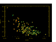
Figure 12: Distributions of cluster X-ray morphology in the Conc-Asym plane. Each cluster point is represented by a X-ray image of the cluster. The X-ray image is identical to the image used for the measurements of morphology.

In Table 2, our morphological measures with 1-sigma error for the entire cluster sample are listed, while Fig. 11 shows the distributions of these measures for the entire sample. An average value for each measure is 0.13, 0.16, 0.22, and 0.05, while median is 0.13, 0.13, 0.21, and 0.04, respectively for Conc, Asym, Elli, and Offcen. Figure 12 shows distributions of cluster morphology in Conc-Asym plane. Each cluster point is represented by an X-ray image of the cluster. The X-ray image is identical to the image used for the measurements of morphology. The same Conc-Asym plot with 1-sigma error is plotted in Fig. 13, together with other measure-measure planes. In Fig. 13, we can see that clusters are scattered and occupying various places in these morphological planes, showing various morphological characteristics. However, there is a weak to strong trend between each set of two measures; the value of Spearman $\rho$ is -0.62, -0.78, 0.39 and 0.79 for Conc-Asym, Offcen-Conc, Elli-Offcen, and Elli-Asym, respectively. The correlation is relatively strong in the Asym-Conc and Offcen-Conc plots. This indicates that low concentration clusters generally show high degree of asymmetry or skewness, illustrating the fact that there are not many highly-extended smooth symmetric clusters. Similarly, a correlation between Asym and Elli may imply that there are not many highly-elongated but otherwise smooth symmetric clusters. The correlation between Asym and Elli is consistent with the power ratio analysis by Buote & Tsai (1996).

Table 2: Morphological measures

Name	Conc	Elli	Asym	Offcen
A3562	0.143$\pm 0.010$	0.152$\pm 0.028$	0.159$\pm 0.012$	0.012$\pm 0.036$
A85	0.161$\pm 0.004$	0.053$\pm 0.013$	0.124$\pm 0.005$	0.039$\pm 0.014$
HydraA	0.171$\pm 0.007$	0.134$\pm 0.022$	0.043$\pm 0.008$	0.003$\pm 0.011$
A754	0.093$\pm 0.004$	0.354$\pm 0.008$	0.323$\pm 0.008$	0.153$\pm 0.032$
A2319	0.105$\pm 0.006$	0.284$\pm 0.021$	0.250$\pm 0.009$	0.098$\pm 0.023$
A3158	0.120$\pm 0.005$	0.216$\pm 0.016$	0.075$\pm 0.007$	0.026$\pm 0.033$
A3266	0.104$\pm 0.005$	0.180$\pm 0.037$	0.296$\pm 0.023$	0.106$\pm 0.021$
A2256	0.098$\pm 0.007$	0.280$\pm 0.025$	0.117$\pm 0.021$	0.129$\pm 0.049$
A1795	0.138$\pm 0.003$	0.130$\pm 0.008$	0.187$\pm 0.004$	0.066$\pm 0.011$
A399	0.100$\pm 0.006$	0.161$\pm 0.026$	0.194$\pm 0.012$	0.102$\pm 0.032$
A2065	0.123$\pm 0.006$	0.309$\pm 0.014$	0.207$\pm 0.010$	0.076$\pm 0.025$
A401	0.118$\pm 0.005$	0.189$\pm 0.023$	0.110$\pm 0.014$	0.054$\pm 0.033$
Zw1215	0.126$\pm 0.012$	0.267$\pm 0.046$	0.110$\pm 0.012$	0.036$\pm 0.022$
A2029	0.161$\pm 0.007$	0.230$\pm 0.026$	0.070$\pm 0.029$	0.018$\pm 0.033$
A2255	0.106$\pm 0.010$	0.235$\pm 0.036$	0.142$\pm 0.025$	0.071$\pm 0.041$
A1651	0.145$\pm 0.011$	0.205$\pm 0.039$	0.098$\pm 0.040$	0.013$\pm 0.029$
A478	0.153$\pm 0.007$	0.211$\pm 0.026$	0.056$\pm 0.007$	0.009$\pm 0.014$
RXJ1844	0.158$\pm 0.044$	0.385$\pm 0.071$	0.202$\pm 0.022$	0.061$\pm 0.019$
A2244	0.140$\pm 0.005$	0.094$\pm 0.014$	0.040$\pm 0.004$	0.008$\pm 0.014$
RXJ0820	0.122$\pm 0.046$	0.044$\pm 0.074$	0.085$\pm 0.024$	0.017$\pm 0.020$
A2034	0.124$\pm 0.008$	0.159$\pm 0.021$	0.120$\pm 0.037$	0.028$\pm 0.042$
A2069	0.127$\pm 0.013$	0.466$\pm 0.033$	0.214$\pm 0.010$	0.036$\pm 0.069$
RXJ0819	0.151$\pm 0.023$	0.083$\pm 0.073$	0.200$\pm 0.019$	0.050$\pm 0.026$
A1068	0.161$\pm 0.010$	0.279$\pm 0.043$	0.076$\pm 0.007$	0.029$\pm 0.011$
A2409	0.131$\pm 0.016$	0.129$\pm 0.054$	0.094$\pm 0.013$	0.041$\pm 0.036$
A2204	0.180$\pm 0.012$	0.090$\pm 0.043$	0.073$\pm 0.009$	0.022$\pm 0.014$
Hercu.A	0.147$\pm 0.012$	0.212$\pm 0.065$	0.073$\pm 0.013$	0.007$\pm 0.021$
A750	0.134$\pm 0.013$	0.141$\pm 0.073$	0.074$\pm 0.043$	0.028$\pm 0.026$
A2259	0.131$\pm 0.019$	0.279$\pm 0.061$	0.126$\pm 0.017$	0.031$\pm 0.040$
RXJ1720	0.158$\pm 0.006$	0.156$\pm 0.023$	0.073$\pm 0.006$	0.018$\pm 0.013$
A1201	0.122$\pm 0.014$	0.457$\pm 0.061$	0.292$\pm 0.011$	0.077$\pm 0.019$
A586	0.144$\pm 0.016$	0.103$\pm 0.056$	0.075$\pm 0.014$	0.018$\pm 0.026$
A2218	0.117$\pm 0.007$	0.160$\pm 0.027$	0.103$\pm 0.008$	0.041$\pm 0.028$
A1914	0.108$\pm 0.006$	0.154$\pm 0.025$	0.113$\pm 0.007$	0.089$\pm 0.029$
A2294	0.132$\pm 0.024$	0.062$\pm 0.074$	0.176$\pm 0.018$	0.064$\pm 0.038$
A1689	0.161$\pm 0.005$	0.177$\pm 0.019$	0.061$\pm 0.007$	0.020$\pm 0.016$
A1204	0.156$\pm 0.011$	0.166$\pm 0.040$	0.049$\pm 0.010$	0.005$\pm 0.013$
MS0839	0.164$\pm 0.015$	0.064$\pm 0.063$	0.078$\pm 0.014$	0.007$\pm 0.015$
A115	0.083$\pm 0.006$	0.153$\pm 0.015$	0.424$\pm 0.010$	0.126$\pm 0.011$
A520	0.086$\pm 0.009$	0.261$\pm 0.027$	0.153$\pm 0.010$	0.157$\pm 0.052$
A963	0.151$\pm 0.008$	0.155$\pm 0.031$	0.080$\pm 0.008$	0.014$\pm 0.015$
RXJ0439	0.185$\pm 0.020$	0.113$\pm 0.060$	0.092$\pm 0.023$	0.018$\pm 0.025$
A2111	0.119$\pm 0.024$	0.302$\pm 0.101$	0.152$\pm 0.018$	0.101$\pm 0.061$
A1423	0.168$\pm 0.022$	0.265$\pm 0.086$	0.114$\pm 0.025$	0.017$\pm 0.032$
Zw0949	0.167$\pm 0.014$	0.243$\pm 0.065$	0.062$\pm 0.013$	0.001$\pm 0.015$
MS0735	0.206$\pm 0.009$	0.259$\pm 0.025$	0.045$\pm 0.009$	0.001$\pm 0.009$
A773	0.121$\pm 0.010$	0.241$\pm 0.038$	0.102$\pm 0.011$	0.030$\pm 0.027$
A2261	0.159$\pm 0.009$	0.143$\pm 0.038$	0.084$\pm 0.010$	0.016$\pm 0.015$
A1682	0.103$\pm 0.030$	0.267$\pm 0.112$	0.349$\pm 0.024$	0.093$\pm 0.081$
A1763	0.123$\pm 0.014$	0.302$\pm 0.050$	0.136$\pm 0.014$	0.036$\pm 0.038$
A2219	0.119$\pm 0.007$	0.389$\pm 0.014$	0.081$\pm 0.006$	0.048$\pm 0.028$
A267	0.128$\pm 0.011$	0.266$\pm 0.041$	0.139$\pm 0.013$	0.023$\pm 0.034$
A2390	0.170$\pm 0.005$	0.301$\pm 0.012$	0.121$\pm 0.005$	0.031$\pm 0.013$
RXJ2129	0.173$\pm 0.016$	0.216$\pm 0.064$	0.093$\pm 0.018$	0.025$\pm 0.025$
RXJ0439	0.147$\pm 0.015$	0.199$\pm 0.047$	0.155$\pm 0.011$	0.037$\pm 0.024$
A2125	0.140$\pm 0.021$	0.289$\pm 0.087$	0.247$\pm 0.014$	0.026$\pm 0.044$
A68	0.131$\pm 0.023$	0.265$\pm 0.057$	0.153$\pm 0.017$	0.058$\pm 0.045$
Zw1454	0.163$\pm 0.006$	0.143$\pm 0.019$	0.074$\pm 0.005$	0.017$\pm 0.008$
A1835	0.170$\pm 0.006$	0.106$\pm 0.018$	0.067$\pm 0.005$	0.022$\pm 0.012$
A1758	0.084$\pm 0.011$	0.472$\pm 0.022$	0.248$\pm 0.010$	0.298$\pm 0.061$
A697	0.123$\pm 0.011$	0.278$\pm 0.039$	0.089$\pm 0.013$	0.019$\pm 0.025$
Zw1021	0.158$\pm 0.007$	0.145$\pm 0.018$	0.117$\pm 0.006$	0.039$\pm 0.013$
A781	0.060$\pm 0.048$	0.215$\pm 0.119$	0.568$\pm 0.026$	0.143$\pm 0.080$
A2552	0.128$\pm 0.020$	0.187$\pm 0.073$	0.140$\pm 0.015$	0.039$\pm 0.028$
A1722	0.127$\pm 0.023$	0.272$\pm 0.058$	0.211$\pm 0.016$	0.079$\pm 0.035$
MS1358	0.177$\pm 0.011$	0.153$\pm 0.031$	0.111$\pm 0.009$	0.021$\pm 0.013$
RXJ1158	0.177$\pm 0.013$	0.217$\pm 0.049$	0.083$\pm 0.013$	0.006$\pm 0.012$
A370	0.113$\pm 0.009$	0.377$\pm 0.026$	0.074$\pm 0.012$	0.039$\pm 0.048$
RXJ1532	0.161$\pm 0.012$	0.180$\pm 0.044$	0.053$\pm 0.012$	0.004$\pm 0.016$
MS1512	0.131$\pm 0.014$	0.176$\pm 0.043$	0.037$\pm 0.015$	0.011$\pm 0.018$
RXJ0850	0.115$\pm 0.015$	0.243$\pm 0.054$	0.144$\pm 0.018$	0.060$\pm 0.034$
RXJ0949	0.145$\pm 0.023$	0.125$\pm 0.052$	0.108$\pm 0.015$	0.035$\pm 0.026$
Zw0024	0.135$\pm 0.037$	0.030$\pm 0.092$	0.184$\pm 0.031$	0.054$\pm 0.025$
RXJ1416	0.136$\pm 0.029$	0.240$\pm 0.081$	0.168$\pm 0.027$	0.056$\pm 0.027$
RXJ2228	0.120$\pm 0.017$	0.215$\pm 0.060$	0.180$\pm 0.019$	0.114$\pm 0.038$
MS1621	0.103$\pm 0.022$	0.153$\pm 0.063$	0.225$\pm 0.016$	0.078$\pm 0.048$
RXJ1347	0.157$\pm 0.005$	0.209$\pm 0.015$	0.110$\pm 0.005$	0.035$\pm 0.013$
RXJ1701	0.171$\pm 0.026$	0.204$\pm 0.076$	0.181$\pm 0.019$	0.041$\pm 0.021$
3c295	0.165$\pm 0.021$	0.039$\pm 0.059$	0.087$\pm 0.017$	0.005$\pm 0.015$

Table 2 (continued)
 
 
  Name Conc Elli Asym Offcen RXJ1641 0.156$\pm 0.032$ 0.194$\pm 0.101$ 0.282$\pm 0.028$ 0.025$\pm 0.031$ CRSSJ0030 0.125$\pm 0.011$ 0.230$\pm 0.013$ 0.256$\pm 0.007$ 0.046$\pm 0.018$ RXJ1525 0.102$\pm 0.022$ 0.309$\pm 0.071$ 0.204$\pm 0.015$ 0.092$\pm 0.051$ MS0451 0.117$\pm 0.008$ 0.263$\pm 0.018$ 0.146$\pm 0.009$ 0.051$\pm 0.029$ MS0016 0.125$\pm 0.009$ 0.190$\pm 0.022$ 0.095$\pm 0.009$ 0.029$\pm 0.026$ RXJ1121 0.100$\pm 0.028$ 0.176$\pm 0.063$ 0.372$\pm 0.013$ 0.086$\pm 0.070$ RXJ0848 0.116$\pm 0.081$ 0.425$\pm 0.127$ 0.185$\pm 0.014$ 0.050$\pm 0.062$ MS2053 0.134$\pm 0.028$ 0.251$\pm 0.096$ 0.135$\pm 0.025$ 0.039$\pm 0.020$ RXJ0542 0.118$\pm 0.019$ 0.295$\pm 0.072$ 0.237$\pm 0.020$ 0.055$\pm 0.042$ RXJ1221 0.117$\pm 0.014$ 0.346$\pm 0.048$ 0.202$\pm 0.015$ 0.091$\pm 0.041$ RXJ1113 0.143$\pm 0.097$ 0.216$\pm 0.137$ 0.121$\pm 0.035$ 0.011$\pm 0.035$ RXJ2302 0.145$\pm 0.036$ 0.065$\pm 0.119$ 0.163$\pm 0.033$ 0.030$\pm 0.027$ MS1137 0.139$\pm 0.012$ 0.089$\pm 0.043$ 0.084$\pm 0.016$ 0.018$\pm 0.020$ RXJ1350 0.115$\pm 0.031$ 0.206$\pm 0.106$ 0.292$\pm 0.017$ 0.086$\pm 0.037$ RXJ1716 0.150$\pm 0.021$ 0.179$\pm 0.100$ 0.131$\pm 0.023$ 0.024$\pm 0.027$ MS1054 0.092$\pm 0.009$ 0.402$\pm 0.024$ 0.296$\pm 0.010$ 0.318$\pm 0.063$ RXJ0152 0.066$\pm 0.013$ 0.585$\pm 0.035$ 0.306$\pm 0.013$ 0.293$\pm 0.060$ WGA1226 0.138$\pm 0.012$ 0.097$\pm 0.041$ 0.103$\pm 0.013$ 0.031$\pm 0.021$ RXJ0910 0.135$\pm 0.000$ 0.163$\pm 0.000$ 0.268$\pm 0.000$ 0.027$\pm 0.000$ RXJ1053 0.085$\pm 0.014$ 0.601$\pm 0.068$ 0.330$\pm 0.008$ 0.174$\pm 0.019$ RXJ1252 0.144$\pm 0.000$ 0.208$\pm 0.000$ 0.184$\pm 0.000$ 0.033$\pm 0.000$ RXJ0849 0.121$\pm 0.021$ 0.113$\pm 0.098$ 0.168$\pm 0.007$ 0.036$\pm 0.067$

Figure 13: Distributions of clusters in various X-ray measure-measure planes with 1-sigma error.

5.3 L-T relation

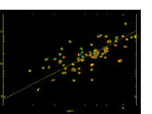
Figure 14: Distribution of cluster X-ray morphology in the L-T plane. The solid line is the fitted line by Wu et al. (1999) based on the local cluster sample.

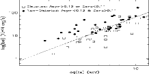
Figure 15: The L-T relation with morphological subsets. The solid ovals are the “non-distorted” clusters and open rectangles are the “distorted” clusters.

Figure 16: Distributions of the shortest distance to the L-T line (LTD) for “non-distorted” and “distorted” clusters.

In Fig 14, we plot a distribution of cluster morphology in the bolometric luminosity (Lbol) and X-ray temperature (Tx) plane using a subset of our sample with available literature data. The straight line is a fit from Wu et al. (1999) based on 256 low redshift clusters in the form of log(Lbol)=2.72log(Tx)-0.92 showing that our sample follows the standard L-T relationship (Spearman $\rho$ = 0.73) with some scatter. To be consistent with the fitted line, here we used H_o=50, $\Omega_{m}$=1, $\Omega_{\Lambda}$=0, cosmology. When we subdivide the sample according to their apparent distortions, using quantitative definition: “distorted” to be Asym $>$ 0.12 or Conc $<$ 0.11, and “non-distorted” to be Asym $<$ 0.12 and Conc $>$ 0.11, and separately plot using open rectangles for the “distorted” clusters and solid ovals for the “non-distorted” clusters (Fig. 15), we see that the distorted and non-distorted clusters occupy well-defined loci in the L-T plane. If we plot distributions of the shortest distance from the point to the L-T line (LTD) in the log(Lbol) and log(Tx) plane for the two subsets (Fig. 16), with positive sign meaning a lower log(Lbol) than the L-T line, we see the same trend. For Fig. 16, a K-S test shows the probability that the two distributions are drawn from the same parent distribution is only 9.56 $\times$ 10^-5. Meanwhile, we do not detect any significant difference in the width of the distributions between two subsets ($\sigma$= 0.078 and 0.081, for the “distorted” and “non-distorted” clusters, respectively).

5.4 Evolutionary effects

Figure 17: Distributions of Lbol for high and low redshift cluster subsets.

To investigate evolutionary effects, we subdivide our sample into low-z and high-z subsets using a border z=0.5. Fig. 17 shows distributions of Lbol for the high-z and low-z samples, while Fig. 18 shows distributions of our measures for high-z and low-z samples. A K-S test shows the probability that the two distributions are drawn from the same parent distribution is 0.01, 7$\times$10^-3, 0.50, and 0.15 for Conc, Asym, Elli, and Offcen, respectively. Table 3 summarizes K-S statistics for various redshift subsets, including the redshift border other than z = 0.5. In Table 3, overall, we see no strong evolution in any of our measures for any redshift subset. There is a hint of weak evolution for Conc and Asym, in such a way that high-z clusters show more distorted morphology, consistent with the sophisticated power ratio method of Jeltema et al. (2005), but it is unfortunately not statistically very significant. Note also that the possible weak trend in Conc becomes increasingly insignificant with the high-z (z$>$0.3) vs. low-z (z$<$0.3) comparison in Table 3.

Table 3: K-S probability with various redshift subsets.

Measure	z$>$0.5 vs z$<$0.5	z$>$0.5 vs z$<$0.3	z$>$0.3 vs z$<$0.3
Conc	0.01	0.03	0.33
Asym	0.007	0.005	0.005
Elli	0.50	0.65	0.50
Offcen	0.15	0.14	0.28

Figure 18: Distributions of various morphological measures for high-z and low-z cluster subsets.

6 Summary and discussions

Using a sample of 101 clusters at redshift z$\sim$0.05-1 taken from the Chandra archive, we quantitatively investigated the relationships between the cluster X-ray morphology and various other cluster characteristics. The X-ray morphology is characterized by a series of objectively-measured simple statistics of X-ray surface brightness, which are designed to be robust against variations of image quality caused by various exposure times and various cluster redshifts.

We found: (1) Our measures are robust against variations of image quality effects introduced by exposure time difference, and various cluster redshifts. (2) The distorted and non-distorted clusters occupy well-defined loci in the L-T plane. (3) Ellipticity and Offcenter show no evolutionary effects between high and low redshift cluster subsets, while there may be a hint of weak evolutions for Conc and Asym, in such a way that high-z clusters show more distorted morphology. (4) No correlation is found between X-ray morphology and X-ray luminosity, or X-ray morphology and X-ray temperature of clusters, implying that interaction of clusters may not enhance or decrease the luminosity or temperature of clusters for extended period of time. (5) Clusters are scattered and occupy various places in the plane composed of two X-ray morphological measures, showing a wide variety of characteristics. (6) Relatively strong correlations in the Asym-Conc and Offcen-Conc plots indicate that low concentration clusters generally show high degree of asymmetry or skewness, illustrating the fact that there are not many highly-extended smooth symmetric clusters. Similarly, a correlation between Asym and Elli may imply that there are not many highly-elongated but otherwise smooth symmetric clusters.

During mergers, clusters are expected to follow a complex track in the L-T plane as shown in several numerical simulations (e.g. Ricker & Sarazin 2001). Meanwhile, simulations by Randall et al. (2002) and Rowley et al. (2004) find that even though the temperature and luminosity of a cluster varies significantly during a merger, it still follows an L $\sim$ T² relation. Apart from simulations, the actual observational evidence also shows mixed results. For example, a study of a ‘major merger’ cluster A2319 (e.g. O’Hara et al. 2004) measuring L & Tx shows little deviation from the self-similar L-T relation, which is consistent with the fact that bulk properties of clusters either do not change much as a result of mergers or change in a correlated way that maintains the small scatter of scaling relations. Meanwhile, a study of ‘merging double’ cluster RX J1053.7+5735 (e.g. Hashimoto et al. 2002) shows significant deviation from the L-T relation.

One of the major problem of these studies is their ambiguous definition of ‘merger’, and resulting heterogeneous sample of dynamically unrelaxed clusters. These results are further complicated by possible bias in measuring L or Tx of clusters with various degree of morphological distortion. For example, Lbol may be systematically underestimated for distorted clusters, because the flux from distorted feature are typically diffuse and extended, and may be excluded from a luminosity measurement using a finite-sized aperture. Tx, on the other hand, can be estimated high without the extended outer part of distorted clusters. Because it is related to the faint signal from the outskirt, these biases can be more prominent in the measurements with small effective area satellites, such as $ROSAT$ and $ASCA$. Similarly, the presence of a ‘cool core’ (e.g. Allen et al. 2001) may bias low the cluster global temperature measurements and/or bias high the cluster global luminosity. If the cool core tends to occur in the dynamically relaxed cluster, the observed trend in Fig. 14, 15, and 16 may partially be the result of this underestimated global temperature and/or overestimated luminosity of the cool core clusters. Indeed, several studies (e.g. Fabian et al. 1994; Allen & Fabian 1998; McCarthy et al. 2004) showed that the clusters with very large values of ‘mass deposition rate’ may preferentially lie on the high-luminosity side of the L-T relation. The cool core clusters may also partially be attributed to the lack of difference in the width of the L-T distributions between the distorted and non-distorted clusters (Fig. 16), because of possible enlarged scatter of the L-T distribution for the non-distorted clusters due to the existence of the cool core clusters (e.g. Fabian et al. 1994; Markevitch 1998; Allen & Fabian 1998; Reichart et al. 1999), while the distorted clusters may intrinsically have the large scatter.

Unfortunately, most of these studies used the mass deposition rate to identify their ‘cooling flow’ clusters. The mass deposition rate is, however, mainly based on the information from the surface brightness profile, roughly equivalent of measuring the morphology of clusters, similar to our concentration index. Thus, previously reported behaviors of the ‘cooling flow’ clusters in the L-T plane may be simply reflecting the ‘morphology effect’ which is qualitatively consistent with our result, and may be showing nothing more than the fact that the clusters with high central surface brightness behave differently from those with low central surface brightness. Indeed McCarthy et al. (2004) reported if they restricted themselves only to the presence of central positive temperature gradient to select their ‘cooling flow’ clusters, the correlation between the presence of the ‘cooling flow’ and the L-T distribution became unclear. Meanwhile studies using simple X-ray core radius of clusters, rather than the mass deposition rate, (e.g. Ota and Mitsuda 2004) reported possible dichotomy in the core radius distribution, which may be consistent with the fact that high central surface brightness clusters behave differently from those with low central surface brightness.

Regardless of the influence of the cooling core, a simple comparison between our morphological measures and the luminosity (or temperature) (Fig. 5 & 6) shows the luminosity or temperature in the literature is not correlated to the morphological measures, indicating that we have no obvious bias in the measurements of L, or Tx for clusters with different degree of morphological distortions. We have also tested systematics for various satellites and various literatures, and found no apparent systematic bias among them.

No matter what causes the shift in the L-T plane, the fact that distorted and non-distorted clusters occupy well-defined loci in the L-T plane demonstrates that the measurements of the global luminosity and temperature for distorted clusters should be interpreted with caution, or alternatively, a rigorous morphological characterization is necessary when we use a sample of clusters with heterogeneous morphological characteristics to investigate the L-T and other related scaling relations. There is much left to learn about the effect of the cluster dynamical state on the bulk properties of clusters of galaxies

Appendix A Derivation of Adaptive Scalings

A.1 Exposure time effect

Intrinsic noise N₀, assuming Poisson noise, contained in the original unsmoothed image I₀ (with background) is:

$$N_{0} = \sqrt{I_{0}}$$ (20)

In the intermediate scaled image I₁ after the scaling, the intrinsic noise contained originally in I₀ will be scaled linearly, and then new Poisson noise will be added in quadrature. Thus the total noise N₁ in the intermediate scaled image I₁ after adding the new noise is,

$$N_{1} = \sqrt{I_{0}I_{1}^{2}/I_{0}^{2}+I_{1}}$$ (21)

$$= \sqrt{I_{1}^{2}/I_{0}+I_{1}}$$

Meanwhile, in the final scaled image I₂, the total noise N₂ will be:

$$N_{2} = \sqrt{I_{2}}$$ (22)

Now, the signal-to-noise ratio in the intermediate scaled image I₁ (after adding the noise) and the final scaled image I₂ should be the same, thus,

$$I_{1}/N_{1} = I_{2}/N_{2}$$

$$I_{1}/\sqrt{I_{1}^{2}/I_{0}+I_{1}} = I_{2}/\sqrt{I_{2}}$$ (23)

Solving for I₁ gives:

$$I_{1} = \frac{I_{0}^{2}I_{2}^{2}}{(I_{0}^{2}I_{2}-I_{2}^{2}I_{0})}$$ (24)

$$= \frac{I_{0}I_{2}}{(I_{0}-I_{2})}$$

However, the scaling from I₀ to I₂ is the scaling factor R₀ described in sec. 4.2.1:

$$R_{0} = I_{2}/I_{0}$$ (25)

$$= t1/t0$$

thus, I₁ can be obtained from I₀ and R₀:

$$I_{1} = \frac{I_{0}I_{0}R_{0}}{(I_{0}-I_{0}R_{0})}$$ (26)

$$= I_{0}\frac{R_{0}}{(1-R_{0})}$$

A.2 Redshift effect

A.2.1 Dimming effect

Intrinsic noise N₀ contained in the original (this time, background subtracted) image I₀ is not proportional to I₀, but proportional to I₀ + B, even if the background B is already subtracted. Therefore, assuming the noise to be Poissonian,

$$N_{0} = \sqrt{I_{0}+B}$$ (27)

In the intermediate scaled image I₁, the intrinsic noise contained originally in I₀ will be scaled linearly, and then new Poissonian noise will be added in quadrature. Thus the total noise N₁ in the intermediate scaled image I₁ after adding the new noise is,

$$N_{1} = \sqrt{(I_{0}+B)I_{1}^{2}/I_{0}^{2}+I_{1}}$$ (28)

Meanwhile, in the final scaled image I₂, the total noise N₂ should include the contribution from the background B, even if the background B is remained subtracted, thus

$$N_{2} = \sqrt{I_{2}+B}$$ (29)

Now, the signal-to-noise ratio in the intermediate scaled image I₁ (after adding the noise) and the final scaled image I₂ should be the same, thus,

$$I_{1}/N_{1} = I_{2}/N_{2}$$ (30)

$$I_{1}/\sqrt{(I_{0}+B)I_{1}^{2}/I_{0}^{2}+I_{1}} = I_{2}/\sqrt{I_{2}+B}$$ (31)

Solving for I₁ gives,

$$I_{1} = \frac{I_{0}^{2}I_{2}^{2}}{[I_{0}^{2}(I_{2}+B)-I_{2}^{2}(I_{0}+B)]}$$ (32)

However, the scaling from I₀ to I₂ is the scaling factor R₁ described in sec. 4.2.2:

$$R_{1} = I_{2}/I_{0}$$ (33)

$$= [(1+z0)/(1+z1)]^{4}$$

thus, I₁ can be obtained from I₀, R₁, and B:

$$I_{1} = \frac{I_{0}^{2}R_{1}^{2}}{[I_{0}R_{1}+B-R_{1}^{2}(I_{0}+B)]}$$ (34)

A.2.2 Angular-size effect

The noise N₂ contained in the dimmed, background re-added, and rebinned image I${}^{{}^{\prime\prime}}_{2}$ is proportional to I${}^{{}^{\prime\prime}}_{2}$. Therefore, similarly to the appendix A.1., the total noise N₃ in the intermediate scaled image I₃ after adding the new Poisson noise will be:

$$N_{3} = \sqrt{I^{{}^{\prime\prime}}_{2}I_{3}^{2}/I_{2}^{{}^{\prime\prime}2}+I_{3}}$$ (35)

$$= \sqrt{I_{3}^{2}/I^{{}^{\prime\prime}}_{2}+I_{3}}$$

Meanwhile, in the final scaled image I₄, the total noise N₄ will be:

$$N_{4} = \sqrt{I_{4}}$$ (36)

The signal-to-noise ratio in the intermediate scaled image I₃ (after adding the noise) and the final scaled image I₄ should be the same, thus,

$$I_{3}/N_{3} = I_{4}/N_{4}$$

$$I_{3}/\sqrt{I_{3}^{2}/I^{{}^{\prime\prime}}_{2}+I_{3}} = I_{4}/\sqrt{I_{4}}$$ (37)

Solving for I₃ gives:

$$I_{3} = \frac{I_{2}^{{}^{\prime\prime}}I_{4}}{(I_{2}^{{}^{\prime\prime}}-I_{4})}$$ (38)

Now, in order to scale the final image I₄ while conserving the surface brightness with respect to the ‘pre-rebinned’ image (i.e. I${}_{2}^{{}^{\prime}}$),

$$I_{4} = I_{2}^{{}^{\prime\prime}}/R_{2}^{2}$$ (39)

thus, I₃ can be obtained from I${}^{{}^{\prime\prime}}_{2}$ and R₂:

$$I_{3} = \frac{I_{2}^{{}^{\prime\prime}}I_{2}^{{}^{\prime\prime}}/R_{2}^{2}}{(I_{2}^{{}^{\prime\prime}}-I_{2}^{{}^{\prime\prime}}/R_{2}^{2})}$$ (40)

$$= I_{2}^{{}^{\prime\prime}}\frac{1}{(R_{2}^{2}-1)}$$

A.3 Combining the exposure and redshift effects

Starting from the equation A.19, namely,

$$I_{3} = \frac{I_{2}^{{}^{\prime\prime}}I_{4}}{(I_{2}^{{}^{\prime\prime}}-I_{4})}$$

Then, unlike the equation A.20, the final image I₄ is now related to the original pre-rebinned image I${}_{2}^{{}^{\prime}}$ by the new factor R₃:

$$R_{3} = I_{4}/I_{2}^{{}^{\prime}}$$

$$= \frac{I_{4}}{I_{2}^{{}^{\prime\prime}}/R_{2}^{2}}=t2/t0$$

So,

$$I_{4}/R_{3} = I_{2}^{{}^{\prime\prime}}/R_{2}^{2}$$ (41)

instead of I₄ = I${}_{2}^{{}^{\prime\prime}}$/R${}_{2}^{2}$ in the Eq. A.20. Thus, I₃ can be obtained from I${}^{{}^{\prime\prime}}_{2}$, R₃, and R₂:

$$I_{3} = \frac{I_{2}^{{}^{\prime\prime}}I_{2}^{{}^{\prime\prime}}R_{3}/R_{2}^{2}}{(I_{2}^{{}^{\prime\prime}}-I_{2}^{{}^{\prime\prime}}R_{3}/R_{2}^{2})}$$ (42)

$$= I_{2}^{{}^{\prime\prime}}\frac{R_{3}}{(R_{2}^{2}-R_{3})}$$

References

- Allen (2000) Allen, S. W. 2000 MNRAS, 315, 269
- Allen & Fabian (1998) Allen, S. W., & Fabian, A. C. 1998, MNRAS, 297, L57
- Allen et al. (2001) Allen, S. W., Schmidt, R. W., & Fabian, A. C. 2001, MNRAS, 328, L37
- Bautz & Morgan (1970) Bautz, L. P., & Morgan, W. W. 1970, ApJ,162, L149
- Böhringer et al. (2000) Böhringer, H., et al. ApJS, 129, 435
- Buote & Tsai (1995) Buote, D. A., & Tsai, J. C. 1995, ApJ, 452, 522
- Buote & Tsai (1996) Buote, D. A., & Tsai, J. C. 1996, ApJ, 458, 27
- Campana et al. (2001) Campana, S., Moretti, A., Lazzati, D., & Togliaferri, G. 2001, ApJ, 560, L19
- Cavaliere & Fusco-Femiano (1976) Cavaliere, A., & Fusco-Femiano, R. 1976, A&A, 49, 137
- David & Kempner (2004) David, L. P. & Kempner, J. 2004, ApJ, 613, 831
- David et al. (1993) David, L. P., Slyz, A., Jones C., et al. 1993, ApJ, 412, 479
- Dressler and Shectman (1988) Dressler, A., & Shectman, S. A. 1988, AJ, 95, 985
- Ebeling et al. (1998) Ebeling, H., Edge, A. C., Böhringer, H., et al. 1998, MNRAS, 301, 881
- Ebeling et al. (2000) Ebeling, H., Edge, A. C., Allen, S. W., et al. 1998 MNRAS, 318, 333
- Edge et al. (1990) Edge, A. C., & Stewart, G. C. 1991, MNRAS, 252, 428
- Edge & Stewart (1991) Edge, A. C., Stewart, G. C., Fabian, A. C., & Arnaud, K. A. 1990, MNRAS, 245, 559
- Ettori et al. (2004) Ettori, S., Tozzi, P., Borgani, S., & Rosati, P. 2004, A&A, 417, 13
- Evrard et al. (1993) Evrard, A. E., Mohr, J. J, Fabricant, D. G., & Geller, M. J. 1993, ApJ, 419, L9
- Fabian et al. (1994) Fabian, A. C., Crawford, C. S., Edge, A. C., & Mushotzky, R. F. 1994, MNRAS, 267, 779
- Gioia et al. (1990) Gioia, I. M., Maccacaro, T., Schild R.E., et al. 1990, ApJ, 72, 567
- Gioia et al. (1999) Gioia, I. M., Henry, J. P., Mullis, C. R., Ebeling, H., & Wolter, A., 1999, ApJ, 117, 2608
- Geller & Beers (1982) Geller, M. J., & Beers, T. C. 1982, PASP, 92, 421
- Gomez et al. (1997) Gomez, P. L., Pinkney, J., Burns, J. O., et al. 1997, ApJ, 474, 580
- Hashimoto et al. (1998) Hashimoto, Y., Oemler, A., Lin, H., & Tucker, D. L. 1998, ApJ, 499, 589
- Hashimoto et al. (2002) Hashimoto, Y., Hasinger, G., Arnaud, M., Rosati, P., & Miyaji T. 2002, A&A, 381, 841
- Hashimoto et al. (2004) Hashimoto, Y., Barcons, X., Böhringer, H., et al. 2004, A&A, 419, 819
- Hasinger et al. (1998) Hasinger, G., Giacconi, R., Gunn, J. E., et al. 1998, A&A, 340, L27
- Henry & Henriksen (1986) Henry, J. P., & Henriksen, M. J. 1986, ApJ, 301, 689
- Henry et al. (1992) Henry, J. P., Gioia, I. M., Maccacaro, T. et al. 1992, ApJ, 386, 408
- Jeltema et al. (2005) Jeltema, T. E., Canizares, C. R., Bautz, M. W., & Buote, D. A. 2005, ApJ, 624, 606
- Jones & Forman (1999) Jones, C., & Forman, W. 1999, ApJ, 511, 65
- Kempner et al. (2003) Kempner, J. C., Sarazin, C. L., & Markevitch, M. 2003, 593, 291
- Kolokotronis et al. (2001) Kolokotronis, V., Basilakos, S., Plionis, M., & Georgabtopoulos, I. 2001, MNRAS, 320, 49
- Markevitch (1998) Markevitch, M. 1998, ApJ, 504, 27
- Mazzotta et al. (2001) Mazzotta, P., Markevitch, M., Vikhlinin, A. et al. 2001, ApJ, 555, 205
- McCarthy et al. (2004) McCarthy, I. G., Balogh, M. L., Babul, A., et al. 2004, ApJ, 613, 811
- (37) McMillan, S. L. W., Kowalski, M. P., & Ulmer, M. P. 1989, ApJS, 70, 723
- Melott et al. (2001) Melott, A., Chambers, S. W., & Miller, C. J. 2001, ApJ, 559, L75
- Mohr et al. (1995) Mohr, J. J, Evrard, A. E., Fabricant, D. G., & Geller, M. J. 1995, ApJ, 447, 8
- (40) O’Hara, T. B., Mohr, J. J., & Guerrero, M. A. 2004, ApJ, 604, 604
- Ota & Mitsuda (2004) Ota, N., & Mitsuda, K. 2004, A&A, 428, 757
- Ota et al. (2004) Ota, N., et al. 2004, ApJ, 601, 120
- Perlman et al. (2002) Perlman, E. S., Horner, D. J., Jones, L. R., et al. 2002, ApJS, 140, 265
- Plionis (2002) Plionis, M. 2002, ApJ, 572, L67
- Press & Schechter (1974) Press, W., Schechter, P. 1974, ApJ, 187, 425
- Randall et al. (2002) Randall, S. W., Sarazin, C. L., & Ricker, P. M. 2002, ApJ, 577, 579
- Reichart et al. (1999) Reichart, D. E., Castander, F. J, & Nichol, R. C. 1999, ApJ, 516, 1
- Reiprich & Boehringer (2002) Reiprich, T.H. & Böhringer, H. 2002, ApJ, 567, 716
- Richston et al. (1992) Richstone, D., Loeb, A., & Turner, E. L. 1992, ApJ, 393, 477
- Ricker & Sarazin (2001) Ricker, P. M., Sarazin, C. L. 2001, ApJ, 561, 621
- Rosati et al. (1998) Rosati, P., Della Ceca, R., Burg, R., Norman, C., Giacconi, R. 1998, ApJ, 492, L21
- Rowley et al. (2004) Rowley, D. R., Thomas, P. A., & Kay, S. T. 2004, MNRAS, 352, 508
- Schindler et al. (1995) Schindler, S., Guzzo, L., Ebeling, H., et al. 1995, A&A, 299, L9
- Schuecker et al. (2001) Schuecker, P., Böhringer, H., Reiprich, T.H., & Feretti L. 2001 A&A, 378, 408
- Vikhlinin et al. (1998) Vikhlinin, A., McNamara, B. R., Forman, W., et al. 1998, ApJ, 502, 598
- Wang et al. (2004) Wang, Q. D., Owen, F., & Ledlow, M. 2004, ApJ, 611, 821
- Wu et al. (1999) Wu, X-P., Xue, Y-J., Fang, L-Z. 1999, ApJ, 524, 22