Field Deployment of Prototype Antenna Tiles for the Mileura Widefield Array–Low Frequency Demonstrator
Abstract
Experiments were performed with prototype antenna tiles for the Mileura Widefield Array–Low Frequency Demonstrator (MWA–LFD) to better understand the widefield, wideband properties of their design and to characterize the radio frequency interference (RFI) between 80 and 300 MHz at the site in Western Australia. Observations acquired during the six month deployment confirmed the predicted sensitivity of the antennas, sky-noise dominated system temperatures, and phase-coherent interferometric measurements. The radio spectrum is remarkably free of strong terrestrial signals, with the exception of two narrow frequency bands allocated to satellite downlinks and rare bursts due to ground-based transmissions being scattered from aircraft and meteor trails. Results indicate the potential of the MWA–LFD to make significant achievements in its three key science objectives: epoch of reionziation science, heliospheric science, and radio transient detection.
Subject headings:
instrumentation: interferometers, site testing, telescopes, radio continuum: general1. INTRODUCTION
With the advent of high-performance, low-cost digital signal processing capabilities, a new approach to radio astronomy instrumentation is possible. At frequencies of a few hundred MHz and below, it has become feasible to directly sample radio-frequency waveforms from antennas and perform traditionally analog functions, such as filtering and mixing, in the digital domain. This minimizes analog devices in the signal path and leads to stable and well-calibrated systems. The low cost of such approaches opens up the possibility of deploying a very large number of small antennas, each equipped with direct-sampling digital receivers, thereby gaining access to seamless, wide fields of view.
Multiple arrays exploiting this new capability are currently under development. These instruments include the Mileura Widefield Array–Low Frequency Demonstrator111http://haystack.mit.edu/ast/arrays/mwa (MWA–LFD) in western Australia, the Low Frequency Array222http://www.lofar.org (LOFAR) in the Netherlands, the Primeval Structure Telescope333Pen et al. (2004) (PAST) in northern China, and the Long Wavelength Array444http://lwa.unm.edu/ (LWA) in New Mexico.
In this paper, we report on a field prototyping effort for the MWA–LFD. This instrument is designed to cover the frequency range between 80 to 300 MHz and will be built at Mileura Station in Western Australia. The site of the MWA–LFD has been chosen as the Australian candidate site for the international Square Kilometer Array (SKA) and efforts are well advanced to establish a radio astronomy park in the region with comprehensive and permanent radio frequency interference (RFI) control measures.
The primary scientific goals of the MWA–LFD are the characterization of redshifted 21 cm HI emission from the cosmological epoch of reionization (EOR) (Furlanetto et al., 2006; Bowman et al., 2006a, b; McQuinn et al., 2006; Wyithe et al., 2005; Babich & Loeb, 2005; Morales & Hewitt, 2004; Zaldarriaga et al., 2004), a survey of the sky for astronomical radio transient sources, and the investigation of the heliosphere through scintillation and Faraday rotation effects in order to demonstrate the ability of such measurements to improve the prediction of space weather (Salah et al., 2005). All of these applications demand very wide fields of view, and as a result, the array design features a large number of small, phased-array antenna tiles with (half maximum) fields of view of deg2, where is the observing wavelength in meters and is in the range m.
The full array will consist of 500 such antenna tiles spread over an area 1.5 km in diameter and will have a total collecting area of order m2 per polarization. Digital receiver units deployed across the array will channelize the sampled data streams from each antenna tile and transmit a selected 32 MHz of sky bandwidth to the central facility at high spectral resolution. At the central facility, all antenna pairs will be cross-correlated in order to avoid multiple layers of beamforming and the consequent boundaries in sky coverage. Application-specific real-time post-correlation processing will be implemented in order to sustain the formidable data rates that will be generated.
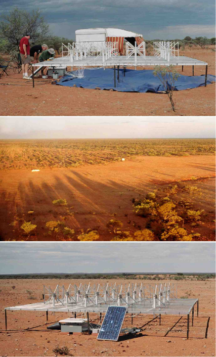
As part of the development effort for the MWA–LFD, prototypes of the antenna tiles were constructed. In order to test these prototypes, as well as to characterize the site for RFI and a variety of environmental factors, we deployed three antenna tiles plus a simple data capture and software correlation system, along with needed infrastructure, at the Mileura site. Four expeditions to the site were conducted from March through September, 2005. During this 6-month period, the equipment was operated for a total of 8 weeks and several terabytes of data were gathered. This program was supported by MIT, the University of Melbourne, the Australian National University, and Curtin University of Technology.
In this paper we describe the prototype system and the results derived from it. In Sections 2 and 3 we describe the equipment and the physical deployment at the Mileura site, along with the experimental results relevant to characterization of the performance of the system. Section 4 addresses site characterization, with particular emphasis on the RFI environment as seen by our systems. In Section 5, a variety of results are presented showing the characterization of astronomical sources with the prototype equipment, and our conclusions are given in Section 6. Two additional astronomical results of independent scientific value regarding Type-III solar bursts and giant pulses from the Crab Nebula pulsar were obtained during the observing campaigns and will be reported separately.
2. INSTRUMENT DESIGN
The basic antenna concept is shown in Figure 1 and is a four-by-four phased-array of wideband active dipoles forming an “antenna tile” operating in the 80 to 300 MHz frequency range. The antenna tile is electronically steerable and, due to the wide frequency range, a switched delay-line beamformer design is employed. The spacing of the dipoles in the four-by-four grid is 1.07 meters, or at 140 MHz. This choice of spacing is aimed at optimizing performance for EOR science, but leads to significant grating lobes at higher frequencies.
The dipoles are a vertical bowtie design, with symmetry above and below the midline in order to minimize horizon gain (see Figure 2). An active balun is located at the junction of the bowtie arms, and the amplified signal is fed to the beamformer unit via coaxial cable. For the prototype units, structural support for these dipole elements was provided by a Lexan tube of 6.25 cm diameter.
Because of imperfect impedance matching between the dipole and the balun, much of the antenna power received from the sky is reflected back to the sky, particularly at the low end of the frequency range. The sky brightness temperature is so much higher than the first-stage amplifier noise temperature, however, that the overall system temperature is dominated by sky noise, despite the loss of the reflected power (see Section 3.2 for additional discussion of the system temperature).
The dipoles need to be positioned over a ground plane, and due to the Lexan tube support structure of the prototypes, it was necessary to construct the ground planes as raised platforms, with a tube clamping arrangement below the conductive screen. This arrangement is visible in Figure 1. Ground planes for each of the three antenna tiles were custom-built, with successive refinements for each ground plane based on experience from the previous antenna tile. For the full array, we expect to use conductive mesh at ground level.
The beamformer units are based on switchable delay lines implemented as coplanar waveguides via traces on printed circuit boards. Switch settings are controlled by a computer workstation communicating with a microcontroller over an RS-232 serial line. Certain beamformer functions, such as power combination, were implemented in the prototype units with commercially built, connectorized modules, and the general degree of component integration was lower than that to be implemented in the full array. However, the prototype beamformer is expected to match the production version closely in performance.
2.1. Wide-band Active Dipole Elements
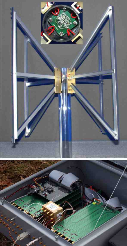

Each dipole element, shown in Figure 2, for the phased-array antenna tile is an “active antenna,” with a low-noise amplifier and a balun integrated into the antenna structure. The combination provides low-noise amplification at the point where the received signal is weakest, and converts it from a balanced to an unbalanced signal, as is necessary before transmitting the signal over coaxial cable to the downstream electronics.
The open-frame, vertical bowtie construction of the antenna elements was chosen with several objectives in mind: wide frequency range, broad angular coverage, low sensitivity at the horizon (to minimize reception of RFI from terrestrial sources), and low manufacturing cost. A simple, horizontal, wire dipole over a ground plane satisfies the latter two, but has difficulties with the first two—especially with a two octave frequency range. The impedance of a dipole has a much stronger frequency dependence than does the input impedance of a typical amplifier. As a result, there is a large impedance mismatch between dipole and amplifier except over a narrow frequency range, and most of the power received from the sky is lost back to the sky. Extending the dipole arms vertically into bowties significantly flattens the frequency dependence of the antenna impedance, thereby improving the match with the amplifier over most of the 80 to 300 MHz range. The conversion to bowties also widens the beamwidth. Constructing the bowtie in outline form, with spars around the outer edges and a single horizontal crosspiece, gives performance similar to a solid-panel bowtie, but with the advantages of reduced wind loading and lighter weight, both of which allow a simplified mechanical support structure and reduce the manufacturing cost.
Each pair of diametrically opposite dipole arms feeds a low-noise amplifier housed in the Lexan tube. The amplifier employs two Agilent ATF-54143 HEMT amplifiers in a balanced configuration with a balun on the output. The amplifier noise temperature is 15 to 20 K (compared with approximately 100 to 5000 K for the sky temperature). The balanced design and intrinsically low distortion characteristics of the HEMT ensure an acceptably low level for any output intermodulation products arising from RFI signals received by the antenna.
2.2. Antenna Tile and Delay-Line Beamformer
For each of the 16 signals of the same polarization from the dipole elements of an antenna tile, the beamformer filters the signal to attenuate out-of-band interference, and then applies a delay between 0 and 10.4 ns, as appropriate to steer the phased-array beam in the desired direction. The delay maximum of 10.4 ns is sufficient to phase the beam to the horizon in the principle planes of the tile, but corner dipoles may be under-delayed in the case of off-axis incident waves with zenith angles greater than 45∘. At a zenith angle of 60∘ and azimuth of 45∘, the corner dipole opposite the reference has a serious delay error of 2.7 ns (0.81 turn at 300 MHz), while the next worst delay errors are only 0.5 ns (0.15 turn at 300 MHz).
The delay for each dipole is generated from five delay lines that may be independently switched in or out of the signal path via paired GaAs switches. The delays differ by powers of two between sections, so the minimum delay step is 0.34 ns, or 0.1 turn at 300 MHz. The coplanar-waveguide construction of the delay lines affords excellent delay repeatability between units and extremely low temperature sensitivity. Following the delay line sections, the signal is combined with the other 15 signals of the same polarization, further amplified, and then sent on to the receiver via coaxial cable.
Each beamformer chassis, shown in Figure 2, contains the delay lines and associated electronics for the two polarizations from a single tile, voltage regulators to step down the DC voltage from an external power source, and a microcontroller-based digital interface to convert RS-232 serial data commands into parallel data. These signals control the delay line switches and also a second set of switches, one per dipole signal, which allow individual dipoles to be switched in or out of the signal path for test purposes or in the event of a dipole failure. During astronomical observations, the control electronics are deactivated to reduce interference except for the brief instants when the delays are reset to change the pointing of the antenna tile beam.
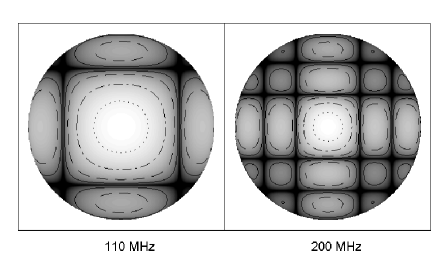
The mutual coupling between antenna elements is less than dB, except between 90 and 140 MHz, where it peaks at about dB at 110 MHz. With this low mutual coupling between antenna elements, the antenna tile power response pattern is modelled as the single-element dipole pattern multiplied by the array factor, which is the pattern the antenna tile would have if all the elements were replaced by ideal, isotropic antennas. The half-power beamwidth of a single dipole element mounted above a ground plane is deg over most of the frequency range, with peak response at the zenith except near 300 MHz. The beamwidth of a full antenna tile varies approximately inversely with frequency, and has zenith values of 15 to 45 deg. The beamwidth increases as the beam is steered down toward the horizon due to foreshortening. Figure 3 shows two example antenna tile power response patterns calculated assuming ideal dipole elements with no coupling. The small actual coupling does cause slight deviations from these patterns, as discussed in Section 3.1.
2.3. Receiver and Digitizer System
For the prototype field deployment, the receiver functions were handled by a simple, dual-frequency conversion system, wherein a 4 MHz band was selected and mixed to 28 MHz center frequency. The signal was digitally sampled at 64 MHz using the “Stromlo Streamer” (Briggs et al., 2006), but only one in four samples was kept, producing an effective sampling rate of 16 MHz.
The system used a computer workstation equipped with a terabyte RAID array to record four input channels at the effective sampling rate with 8 bit precision, giving a data rate of 64 MB/s that was recorded to disk. Normally, only the low order bits were toggled by the received signals. The dynamic range of the 8 bits allowed operation of the system over the full frequency range without further gain adjustment. There was ample head-room for RFI signals, and in those few instances where higher order bits were needed, the IF conversion system entered a non-linear regime due to the high signal power concentrated in the 4 MHz passband at the output of the IF system. The data were processed in software by playing the recordings back into an FX correlator code which computed both auto- and cross-correlation power spectra. There were two principal modes of operation: a high spectral resolution mode, which implemented a polyphase filter bank to obtain 1 kHz spectral channels with a high level of channel-to-channel rejection, and a 16 kHz resolution mode, which used a straight FFT for spectral dispersion in order to cut the correlation time to a little longer than recording time. This latter mode produced 512 channels and was used in the analysis in Section 5.2.
2.4. Array Layout
The location of the prototype deployment array is given in Table 3. At the site, the three antenna tiles were deployed in a triangular configuration roughly 300 m across, as illustrated in Figure 4. This provided interferometer baselines of sufficient length to resolve out the diffuse galactic emission and to effectively isolate signals from bright individual point sources through phase-stable interferometry. The configuration also allowed the potential of the array to yield scientifically interesting astronomical information.
2.5. Site Infrastructure
The prototype field deployment campaigns had modest infrastructure requirements. A small caravan (trailer) was purchased and placed on-site to act as the control center and house the receivers and computer equipment. Battery-backed solar power units were installed to power each of the three antenna tiles and a portable diesel generator was used at the caravan to provide power for the electronics and daytime air conditioning. Coaxial cables of 200 m length were used to transport signals from the antenna tile beamformers to the caravan, and the cables were simply laid on the ground. Between campaigns, the beamformers and solar power units were removed and placed in storage.
3. CALIBRATION AND PERFORMANCE
3.1. Antenna Power Response Pattern
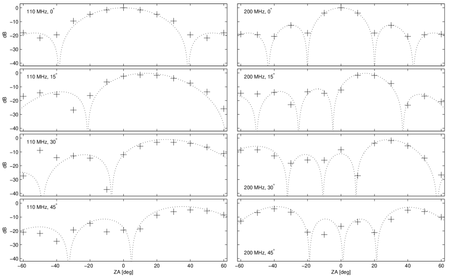
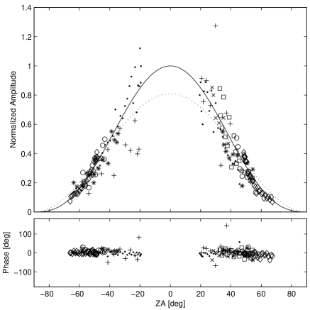
The actual antenna power response pattern for the prototype antenna tiles was constrained using two methods. Prior to installing the antenna tiles in the field, the response function was determined at two frequencies by systematically scanning a transmitter above an antenna tile using facilities at the MIT Haystack Observatory. Figure 5 shows resulting beam profiles for line scans in the E-plane of the antenna tile at four different antenna tile pointing angles. The structures in these profiles agree well with the patterns produced by assuming that the antenna tiles consist of ideal dipole elements above an infinite ground plane with no mutual coupling, which are shown as the dotted lines in Figure 5. There are a few notable deviations. Most prominently, the primary beam appears larger than predicted at 110 MHz, as can be seen in the upper-left two panels in the Figure. Additionally, the nulls in the beam patterns are not as deep as would be expected from the ideal calculations, and at the larger pointing angles, there are some significant deviations from the expected patterns. Some of these discrepancies may be the result of the test conditions. The distance (15 m) between the transmitter and antenna tile was not sufficient to reach fully the far-field limit for the radiation patterns, and the alignment and pointing of the transmitter at the antenna tile was performed manually with an estimated margin of error of in each, allowing ambiguities in the effective zenith angle and in gain due to the dipole pattern of the transmitter.
In the field, additional measurements were achieved by interferometrically isolating point sources and tracking them as they drifted across the sky. This technique effectively separated the dipole element power response pattern from that of the full antenna tile pattern and resulted in an estimate of the effective dipole power envelope as a function of zenith angle. The amplitudes of the interferometrically isolated point sources were fit to a profile, where is the zenith angle and is a constant. The best-fit at 120 MHz is shown in Figure 6 and was found to be given by , whereas an ideal dipole has and is excluded by the measurements at the 85% confidence level. This indicates that the effective power pattern for the antenna tile dipole elements has a somewhat narrower shape than the ideal case.
3.2. Gains and System Temperatures
The gain and noise temperature of an antenna tile system was measured by setting its beamformer delays to point the antenna tile towards zenith and then recording the signal over a long period of time as the Earth turns and the beam transits the Galactic plane. In this technique, the measured power is compared to the predicted power by convolving a map of the low frequency Galactic synchrotron emission with the computed antenna power response function. The data are fit by (Rogers et al., 2004, Their Equation 1),
| (1) |
where is the measured power in arbitrary units as a function of local sidereal time (LST), is the receiver gain, is the sky model as function of direction in the sky , is the antenna power response pattern, includes the remaining system noise contributions (including amplifier noise and ground spillover) referred to the antenna output, and is the convolution operator.
We used the 408 MHz sky map made by Haslam et al. (1982) and assumed a spectral index of to extrapolate to the observed frequencies. The power response pattern for the prototype antenna tiles was taken to be that of ideal dipole elements with no mutual coupling above an infinite ground plane, as described at the end of Section 2.2. Although this simplified model was shown in Section 3.1 to produce a larger dipole power envelope than that of the actual antennas tiles, it deviates by only approximately 10% at the edge of the primary antenna tile beam when phased to the zenith.
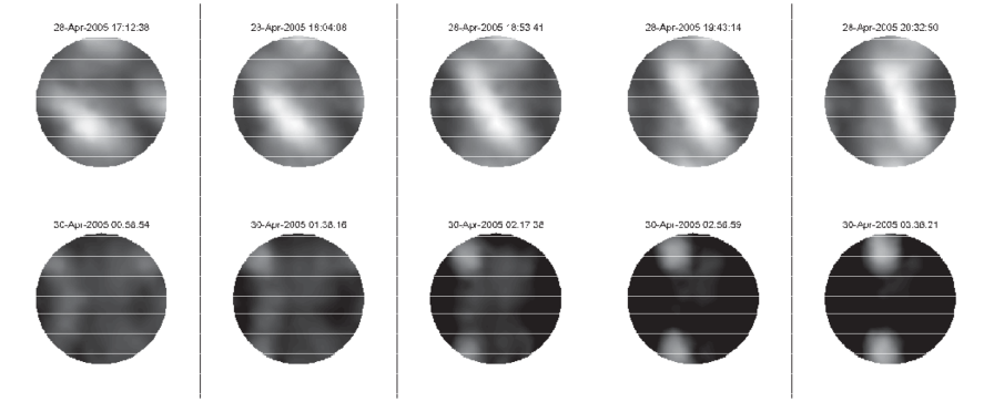
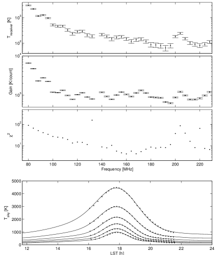
Figure 7 gives examples of the actual sky as seen by a prototype antenna tile, and Figure 8 shows the results of the system gain and noise temperature calibration between 80 and 230 MHz. In general, the effective receiver temperature as measured at the output of the antenna was found to be below about 200 K except at the lowest frequencies measured, although, the results are considered a lower limit on the performance of the system due to an equipment problem at the time of the observations which increased impedance mismatches within the beamformer of the antenna tile used for the observations. The predicted antenna temperature as a function of LST and examples of the best least-squares fits of the data at six frequencies are also given.
3.3. Baseline Determination
Baselines of the final array configuration were determined using observations of unresolved astronomical continuum sources. The antenna coordinates were defined in the conventional right-handed, cartesian coordinate system with the - and -axes lying in a plane parallel to Earth’s equator and the -axis parallel to Earth’s rotation axis pointing towards the north pole. In terms of hour angle (HA) and declination (Dec), , , and are measured towards (HA = 0h, Dec = 0∘), (HA = -6h, Dec = 0∘) and (Dec = 90∘) respectively. In this coordinate system, a large HA coverage is useful to constrain the and components of the baseline, and the component is best constrained by observing sources spanning a large range in declination.
An observing session optimized for baseline calibration was conducted on the night of September 15, 2005 which continued through mid-morning the next day. The observations were carried out at 120 and 275 MHz using the north-south aligned polarization on all three tiles and observed seven bright, unresolved sources: Tau-A, Her-A, 3C252, 3C161, Pic-A, PKS 2152-69 and PKS 2356-61. The relative antenna tile locations are given in Table 1, and Table 2 shows a comparison between the baseline vectors determined by astronomical observations and those obtained manually by using a tape measure.
The resulting antenna tile positions are sufficiently accurate to correct the interferometer phases for changing geometrical delays as a function of hour angle and declination. The least square fitting uncertainties in and were determined to be about 2 cm and those in to be about 5 cm. The dominant sources of error in the antenna tile coordinates due to pseudo-random effects were cross talk in the receiver chains (see Section 3.5) and ionospheric variations (see Section 5.2.1).
3.4. Antenna Delays
In addition to determination of the antenna coordinates, calibration of interferometric data requires the determination of antenna based delays (or phase offsets) due to differences in the electrical path lengths to different antennas. These offsets were determined using observations of Pic-A conducted on September 18, 2005. An analysis using all three baselines sensing the east-west aligned polarization led to the conclusion that the electrical paths to antenna tiles 1 and 2 differ by 1.5 m and that those to antenna tiles 1 and 3 differ by 0.6 m. The major contributor to these difference is differing lengths of the cables between the antennas and the inputs to the digitizers. The measured instrumental phase offsets were found to be well behaved, varying with frequency as where is the electrical path difference and is the speed of light.
3.5. Cross Talk
When the array was pointed at a bright radio source, the interferometers showed a response with two components: one corresponding to the natural fringe rate due to the Earth’s rotation, and a second that was invariant with time. Due to the simplicity of the receiving system, it was deduced that the invariant component is dominated by an instrumental component, caused by cross talk (faint electrical coupling) between the signal paths in the receiving system. In more sophisticated receivers, this effect can be avoided by phase switching the signal close to the antenna, followed by synchronous demodulation in the digital section, and the full array will employ this technique.
For the purposes of this prototyping exercise, it was sufficient to approximate the invariant term by a long average of the interferometer response at “zero fringe rate” (i.e., computed without compensation for Earth rotation) and to remove the cross talk component by subtraction of the average from the visibility data prior to application of the fringe de-rotation for the celestial sources.
3.6. Noise and Integration Time
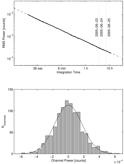
In order to assess the noise characteristics of the system, a deep integration was acquired in an empty part of the spectrum with one antenna tile. The observation was conducted over three days beginning June 23, 2005, and resulted in 10 h of total integration in a 4 MHz band centered at 187 MHz with 1 kHz spectral resolution. The integration was processed to remove the bandpass and corrected for amplitude variations due to variations in Galactic noise with LST. From these cleaned data, 1000 contiguous channels spanning 188 to 189 MHz were selected and analyzed as a function of the cumulative integration time. For pure thermal noise, the variation of the individual channel powers about the mean should have a Gaussian distribution and their RMS should be proportional to the inverse square root of the integration time (). Figure 9 shows that the observed trend is consistent with thermal noise and that the distribution of channel powers at the end of the integration is approximately Gaussian.
4. SITE CHARACTERIZATION
The Mileura site is a new venue for radio astronomy and the prototype field deployment system was one of the first instruments to be deployed at the site. The effort, therefore, was able to provide valuable experiences regarding working conditions in the remote area, the ability of the equipment to withstand the harsh environment, and the suitability of the site for low frequency radio astronomy. In this Section, we report significant findings on these topics.
4.1. The Mileura Environment
Mileura Station is an active sheep and cattle station (ranch) in a remote area approximately 620 km north of Perth, Western Australia. The nearest towns are Meekathara (100 km east) and Cue (150 km southeast), and the nearest small city is Geraldton (350 km southwest). During dry seasons, Mileura can be reached from Perth by car or truck in approximately 10 hours over paved and dirt roads. In wet weather, the dirt roads may become virtually impassable for short periods of time, cutting off access to the site. The ranch consists of about 620,000 acres (2500 km2) of natural grazing land for sheep and cattle, but kangaroos, emus, feral goats, lizards, snakes, birds, and many insects are also abundant. The climate of the region is arid (see Table 4).
Prominent concerns prior to the field deployment effort regarded the logistics of working at the site and whether the equipment would be able to endure the harsh environment, including the climate and the wildlife. Over the course of the six-month deployment, the equipment was operated successfully in a variety of conditions including extreme heat, severe winds, cool nights, and light rain. Additionally, although numerous kangaroos and emus were seen in the vicinity of the array, no damage or evidence of any interaction with the equipment was observed.
Several severe storms occurred while the array was not in use. One of these storms produced flooding at the site. Inspection of the antenna tiles after the flooding showed clear signs that running water passed under the elevated ground planes, eroding material around the ground plane supports. A second storm produced large hail (up to 3 cm in diameter) at the site, but no significant damage was detected to the antenna tiles, including the dipole elements and ground planes.
4.2. Radio Frequency Interference
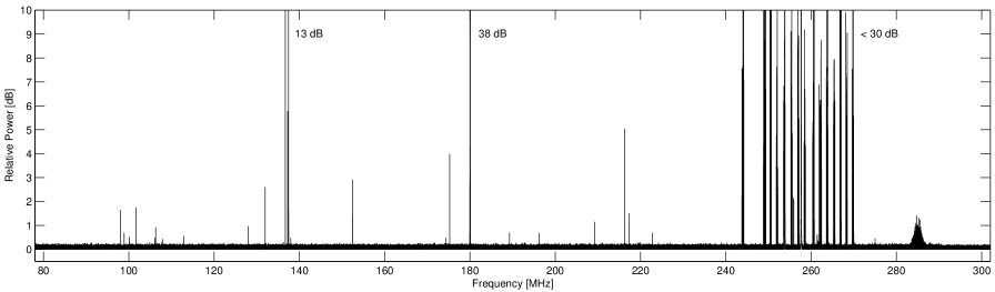
Characterizing the RFI at the Mileura site was an important objective of the prototype field deployment effort and a significant amount of observing time was dedicated to this task. All RFI studies were processed with the high spectral dynamic range, polyphase filter bank mode to obtain 1 kHz resolution. Figure 10 gives an overview of the strongest signals in the 80 to 300 MHz band. This full spectrum scan results from the stitching together of a sequence of 4 MHz bands. Each individual band was observed for 15 seconds by a single antenna tile phased to point at the zenith and was bandpass corrected. With 1 kHz channels, less than 1% of the spectrum was occupied by interferers above 5- in this observation. The strongest identified features, most notably at 137, 180, and 240 through 270 MHz, originate from satellites. The temporary receiving system used in these prototyping exercises emits signals at multiples of the 64 MHz sampling clock that could be detected in the deep spectra. The full array will use a much higher sampling rate, and the critical components will be contained in RFI tight enclosures.
4.2.1 Long Integrations
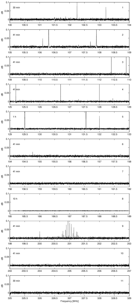
Figure 11 shows spectra for long integrations in 11 selected bands. The observations vary between 30 min and 10 h and each was acquired with a single antenna tile phased to point at the zenith. The sensitivity levels probed with these deep integrations, where the time-bandwidth product is -, achieve RMS channel powers more than 30 dB below the galactic background at 1 kHz resolution. These observations illustrate that the spectrum is remarkably free of RFI.
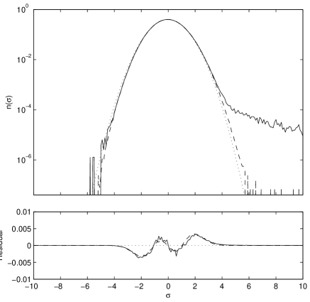
The RFI in a particular observation can be characterized by considering the histogram of individual 1 kHz by 1.3 sec samples comprising the full integration. Absent of RFI and systematic processing errors, the distribution of samples should approach a Gaussian distribution. Figure 12 shows two such histograms for the 42 min and 10 h observations centered at 107 and 187 MHz, repsectively (panels 2 and 8 in Figure 11). The significant presence of RFI due to FM radio transmissions in the observation centered 107 MHz is quite clear as a deviation above a pure Gaussian distribution at high , while the very clean spectrum around 187 MHz reproduces a Gaussian distribution more accurately. In both cases, there appears to be a slight systematic deviation (shown by the bottom plot in Figure 12) from the best-fit Gaussian at all levels. The deviation is most likely an artifact of the bandpass correction applied to both observations.
The 10 h integration centered at 187 MHz (also discussed in Section 3.6) is a particularly clean observation and has significant implications for the measurements of redshifted 21 cm HI emission that will be targeted by EOR experiments with the full MWA–LFD. The planned EOR observations will require very deep integrations, of order 100 to 1000 h, to achieve the required sensitivity levels. The duration of the observation centered at 187 MHz, therefore, represents a substantial step towards characterizing the properties of the RFI at levels approaching those of interest, and the lack of detectable interferers (even if over only a small portion of the total spectrum) bolsters confidence that the full MWA–LFD will be able to achieve the very deep integrations needed to detect evidence of fluctuations in the redshifted 21 cm HI emission from the EOR.
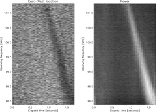
4.2.2 Reflections from Meteor Trails and Aircraft
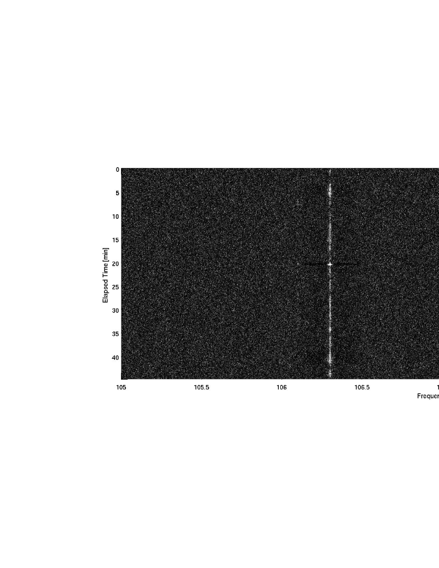
The strong interferers at the frequencies of greatest interest for EOR experiments (below 200 MHz) tend to be highly time variable. Figure 13 presents a dynamic spectrum or “waterfall” plot in order to illustrate the time variability of signals in the portion of the FM band between 105 and 109 MHz. Two consistent interferers with variable amplitudes are observed at 106.3 MHz and 107.9 MHz, and are typically detected at 15- in 1 kHz channels with 1.3 sec integrations. Figure 13 also contains two events at approximately 7 min and 20 min elapsed time when the power in individual frequency channels, including many outside the consistent carrier channels, deviates by up to 20 dB, or well above 100-. Much of the power in the interferers in the FM band is from short-duration bursts like these. The two interferers visible in the top panel in Figure 11 are due entirely to short-duration events, and the peak at 112.4 MHz in the third panel is significantly dominated by another two such events, one of which increases the power in the peak channel by 25 dB.
These events are believed to be due to radiation from distant, over-the-horizon transmitters scattering off the plasma in meteor trails toward the array (Yellaiah et al., 2001; Mallama & Espenak, 1999). Meteoroids enter the Earth’s atmosphere at speeds of order 10 km s-1 and ablate significantly around 100 km altitude. The ablated atoms interact with molecules in the atmosphere producing meteor trails, expanding clouds of plasma. Radio reflections can be produced from radiation scattering off the plasma immediately surrounding the moving meteoroid or off the trail. Scattering events from the vicinity of the moving meteoroid are very brief, sec, while scattering from meteor trails last generally around one second (although some may persist for minutes).
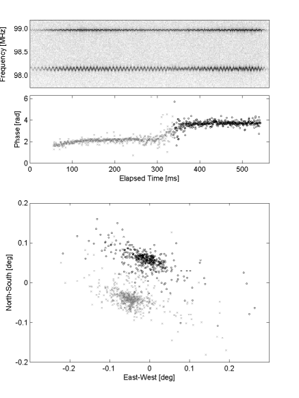
Figure 14 shows a high time resolution measurement of a meteor trail event in which carrier waves from two distant transmitters are briefly visible and seen to modulate with their audio signals. All three antenna tiles recorded this event with sufficient signal to noise that interferometric phases were available. Solving for the centroid of the reflected radiation (Figure 14, bottom panel) reveals two distinct distributions separated by approximately 0.1 deg. At an altitude of 100 km, this angular separation corresponds to an offset of about 175 m. The two distributions are divided in time, as well, with one coming from the first 300 ms of the event and the other from the final 200 ms. The transition between the two features lasts approximately 50 ms. This is consistent with observing the transition from “head” scattering due to plasma immediately surrounding the meteoroid as it enters the atmosphere to trail scattering due to the lingering partially ionized cloud that forms in its wake (Close et al., 2002).
The metallic surfaces on aircraft are also capable of reflecting distant transmissions toward the array. Unlike meteoroids entering the atmosphere, aircraft are typically moving at speeds of order 0.2 km s-1 at altitudes around 30 km; and the rounded surfaces on aircraft may favorably reflect radiation for up to a few minutes as the aircraft moves across the sky.
The sporadic nature of the FM signals detected with the prototype system appears largely to be due to scattering from meteor trails and reflections from the metallic surfaces on aircraft. Overall, ten unique transient events were recorded in the FM band during 2 h of discontinuous observing. There were seven events lasting less than 3 sec, one event lasting 40 sec, and two events lasting about 65 sec. The lengths of these events suggest that the seven short-lived reflections are due to meteor trail reflections and the three longer events are most likely due to aircraft reflections. The total temporal occupancy was about and the spectral occupancy during the events increased by as much as a factor of 100 from to over a 4 MHz band.
Since the integrated spectrum in the FM band is dominated by meteor reflections that have very low temporal occupancy, the implication is that whatever RFI exists in other bands (even well below the sensitivity threshold achieved in extended integrations by the prototype system) may be similarly dominated. It may be possible to eliminate most of the weak RFI in other bands by full-band excision of time slots when the FM band is observed to contain strong reflections from over-the-horizon interferers. Using such a scheme, the MWA–LFD should be able to go much deeper than the -30 dB achieved with the prototype system, without picking up any significant interference.
5. OBSERVATIONAL RESULTS
5.1. Fornax A Imaging
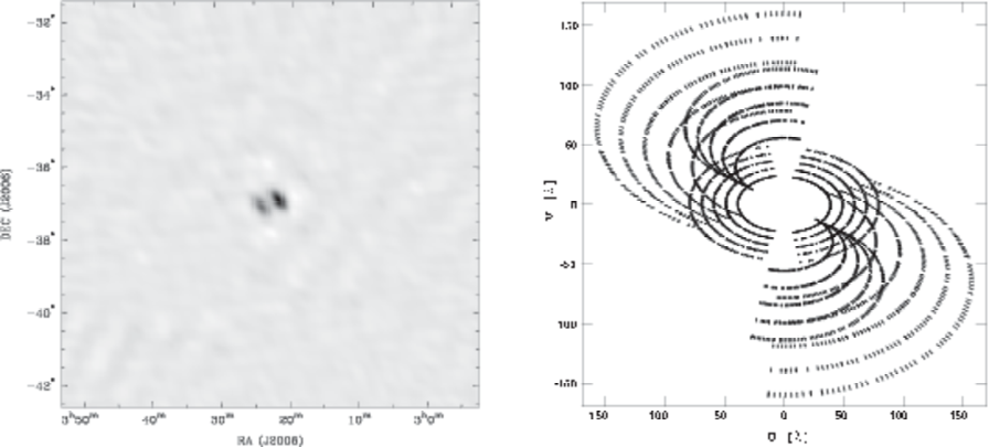
As a final test of the stability of the prototype system and of our consequent ability to achieve consistent amplitude and phase calibration over both time and frequency, it is useful to attempt imaging observations of bright, discrete radio sources. We have done this for the well-known source For-A (R.A. 03h 22m 40s, Dec. -36∘ 14’ 20”), which has a prominent double morphology of 50 arcmin angular extent, sufficient to be resolved by the prototype array. The total flux density of For-A is 475 Jy at 150 MHz, rising to 900 Jy at 80 MHz (Ekers et al., 1983).
Data were acquired on September 18, 2005, using 4 MHz bands centered at 80, 100, 120, 140 and 160 MHz. The observations cycled between these and other frequencies every 7 minutes over a period of 10.5 hours, with an on-source integration duty cycle of roughly 3.3% at each frequency. The data were correlated on-site using the 512-channel mode and the resulting visibility measurements were stored for later analysis.
The For-A dataset included regular observations of Pic-A, which is not resolved by the prototype system interferometers. The observations provided the gain and phase calibration required in addition to that needed for the baseline determination (see Section 3.3) used to correct for geometric delay and Earth rotation. We also calculated the cross-talk contribution from the data itself and subtracted it before exporting the data to FITS files for subsequent analysis and imaging.
Team members experimented with creating images in several imaging packages. This included the use of self-calibration to correct phases. All single-frequency images showed clear double structure, but due to the sparse visibility coverage in the -plane from only 3 baselines, strong residual sidelobe structures were widespread.
In order to improve the image quality, we obtained more complete -coverage by implementing “multifrequency synthesis” (Sault & Conway 1999). The Miriad package turned out to be the most convenient environment in which to perform this task. The multifrequency synthesis algorithm in Miriad generates both an intensity and a spectral index map of the source, in effect scaling the visibilities to a compromise flux scale. The formal dynamic range of the resulting image in Figure 15 is 100:1 (peak/rms), and the observed structure is in excellent agreement with high fidelity images of Fornax A at higher frequencies (Jones & McAdam, 1992; Fomalont et al., 1989).
This successful mapping exercise indicates that the calibration of the prototype antenna tiles and receivers is reasonably well understood. There are various effects which will limit the fidelity of the image shown in Figure 15, including unmodelled spectral gradients in the For-A structure, unmodelled time-variable instrumental response to any linearly polarized emission in For-A, and the presence of other sources within the antenna tile field of view. Of these, the biggest source of uncertainty is most certainly the cumulative effect of other sources entering both the main beam of the antenna tile and the strong sidelobes, which, in some cases, are only dB below the peak response (see Figure 5). There has been no attempt to perform an all-sky self-calibration or source subtraction in order to achieve a more global solution.
5.2. Solar and Ionosphere Measurements
During September 12 through 21, 2005, the Sun was observed in an 8 MHz band centered at 100 MHz for several hours per day. The data collection mode consisted of an alternating pattern of observing for 64 contiguous seconds and then calculating the auto- and cross-correlations for all three antenna tiles for a similar amount of time. This resulted in an approximately 50% duty cycle. To maintain a high time resolution in the processed data while minimizing the downtime for computation, the 512-channel correlator mode was used to produce 16 kHz-wide frequency channels. The resulting spectra were saved with 50 ms temporal resolution.
A single, large cluster of sunspots, NOAA active region 0808, was present on the Sun during the entire prototype field deployment (March through September, 2005) and was the source of all flares occurring during the deployment (flare information courtesy of the NOAA Space Environment Center555http://sec.noaa.gov/). During periods when no sunspots were visible on the solar surface, such as on September 20, 2005, the measured fluxes at 100 MHz from the Sun were Jy.
On September 16, 2005, an M4.4-class flare commenced at 01:41 UTC from active region 0808. The active region was located at S11W26 on the solar disk. The x-ray flux peaked at 01:49 UTC and decayed to 50% peak intensity by 01:56 UTC. Observations with the prototype equipment began at 02:00 UTC and covered the subsequent hour as the flare continued to decay. In contrast to observations of the quiet Sun, the measured background power at all frequencies in the 8 MHz band during this period was elevated by a factor of 40, with typical values of Jy.
Dozens of short duration radio bursts were observed during this period. The bursts had durations of 0.5 sec or less in any one frequency channel, descended rapidly across the observing band to low frequencies within seconds, and had peak power levels that could exceed Jy. These are signatures of Type-III solar radio bursts, which are generated by beams of electrons travelling along magnetic field lines at speeds above 20,000 km s-1 (Benz, 2002; Cairns & Kaiser, 2002).
In Type-III solar radio bursts, the motion of the electrons along the field lines excites fluctuations in the corona at the local plasma frequency, and these fluctuations are converted into radio emission at the plasma frequency or at a harmonic. As the electrons escape along an open field line into interplanetary space, the density of the local plasma decreases, resulting in a rapid drop in the emitting frequency. Figure 16 (right panel) shows the measured power as a function of frequency and time for a clear Type-III burst observed by the prototype system.
A more detailed study of the properties of the individual radio bursts will be the subject of a future paper. In the remainder of this section we examine the variation of the location of the emission centroid.
5.2.1 Emission Centroid
Since both the bursts and the background solar emission were very intense during the flare on September 16, 2005, each individual frequency and time interval had sufficient signal to noise to solve for the unique location of the centroid of emission using the phases of the cross-correlated powers. In general, the combination of the three baselines produced locations repeatedly to within 10 arcsec.
Two forms of variation were seen. On a timescale of several hundred seconds, the location of the centroid for the Sun wandered by about 7 arcmin, much larger than the error in the solutions for the emission location. Intense radio bursts were associated with sudden deflections in the source location, as can be seen in Figure 16 (left panel). We attribute the long-term motion to small changes in electron column density between each antenna tile and the Sun due to density gradients in the ionosphere; whereas the short term change in the emission centroid is believed to be due to the burst region itself. If the burst region is slightly offset from the location of the background emission and momentarily dominates the power along the baselines of the array, the location of the centroid will move during the bursts.
Figure 17 is a plot of the location of the emission centroid as a function of wavelength for one snapshot interval without radio bursts. The absolute location is unknown due to uncertainties in the lengths of the cables between the antenna tiles and other experimental effects, but there is a clear gradient in any given interval between displacement and wavelength. A simple model for the angular offset, , that one would expect with wavelength due to a difference in electron column density in the ionosphere between the antenna tiles is given by:
| (2) |
where is the difference in the total electron content (TEC), is frequency, and is the length of the baseline. Although the observed frequency band was too narrow to clearly see the dependency expected from Equation 2, the properties of the centroid displacements were consistent overall with the effects of ionospheric gradients, as opposed to poor calibration of the baselines, since they exhibited quasi-random behavior as a function of time. For the observation shown in Figure 17, we identify a best-fit value for the of electrons m-2. This is several thousand times smaller than the typical total electron content for the daytime ionosphere.
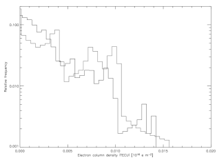
We quantify the ionospheric variation associated with the long-term (several hundred second) variation in the location of the emission centroid in Figure 18, which shows a histogram of the relative frequency of occurrence of different values of the differential electron column density between the antenna tiles. For the one hour period analyzed, 90% of the time the difference in TEC was less than 0.005 TECU, where 1 TECU electrons m-2 This distribution should represent a relatively extreme case since the ionosphere was active during this period, as a coronal mass ejection associated with a flare several days earlier had arrived recently at Earth and triggered a geomagnetic storm.
5.2.2 Implications for Ionospheric Calibration
As demonstrated by Figure 17, the apparent positions of astronomical sources on the sky shift due to variations in electron column density over the array. These positional errors will contribute to the noise levels in MWA–LFD images and uncertainties in EOR statistical measurements, thus their calibration and removal over the wide field of view will be a critical component of the final image processing path for the full MWA–LFD. With the antenna tile characteristics measured during the prototype field deployment, quantitative estimates of the efficacy of the planned ionospheric calibration can be made.
Simulations of the ionospheric calibration process for the full MWA–LFD have been performed and will be described in detail in a future paper. The simulated technique is based on algorithm that is used for Very Large Array data taken at 74 MHz (Cotton et al., 2004; Lane et al., 2004; Cohen et al., 2004), where the longer baselines and lower frequency make ionospheric calibration much more challenging than for the MWA–LFD case. For a model ionosphere whose electron column density fluctuations are comparable to those determined in Section 5.2.1 (as shown in Figures 17 and 18), a 9th-order two-dimensional polynomial fit to the measured offset in the locations of 160 predetermined calibrator sources results in RMS residuals in position of 4 to 6 arcsec (2 to 3% of the 200 MHz array beam) over an 8∘ by 8∘ field of view. The residual noise level was Jy, equivalent to the thermal noise level that would be reached by the MWA–LFD in h of integration. Although the field of view of the actual array will be greater than 20∘ by 20∘ for frequencies below 200 MHz—and the model fit would be according less accurate given the same number of calibrator sources and order of polynomial—with refinement it is projected that ionospheric calibration will not limit MWA–LFD image fidelity or significantly interfere with EOR statistical measurements.
6. CONCLUSION
The design of the MWA–LFD is a departure from traditional approaches to radio astronomy instrumentation. The wide field of view and large bandwidth coverage of the instrument, combined with the phased-array design of the antenna tiles and low-cost digital receiver system, create exciting new opportunities for scientific exploration in a part of the electromagnetic spectrum that has been largely neglected for decades. But for the array to fully succeed in achieving its science objectives requires an understanding of the operational properties of the instrument at unprecedented levels.
The field testing campaign reported on here was conducted to begin addressing this requirement at an early stage in the development of the array. The results of the effort demonstrated the fundamental performance of the MWA–LFD prototype antenna tiles and receiver system in the Western Australia environment. The experiments further indicated that the RFI environment of the site is excellent and should not pose a significant hurdle for the planned observations, including those targeting the epoch of reionization.
Analysis of the data obtained with the prototype system confirmed the presence of several Type-III solar bursts during the field campaign and probed their spectral, temporal, and spatial structure; constrained the properties of the local ionosphere during a period of high solar activity; and detected several bright giant pulses from the Crab Nebula pulsar. These results are all relevant to active fields of study and provide enticing precursors of what will be achievable with the full array.
References
- Babich & Loeb (2005) Babich, D., & Loeb, A. 2005, ApJ, 635, 1
- Benz (2002) Benz, A. O. 2002, Plasma Astrophysics (2 ed.) (Kluwer, Dordrecht)
- Bowman et al. (2006a) Bowman, J. D., Morales, M. F., & Hewitt, J. N. 2006a, ApJ, preprint (astro-ph/0512262)
- Bowman et al. (2006b) Bowman, J. D., Morales, M. F., & Hewitt, J. N. 2006b, ApJ, 638, 20
- Briggs et al. (2006) Briggs, F. H., Torr, G., Campbell-Wilson, D., Blake, A., & Kalnajs, A. 2006, in preparation
- Cairns & Kaiser (2002) Cairns, I. H., & Kaiser, M. L. 2002, in The Review of Radio Science 1999-2002, ed. W. R. Stone (Wiley-IEEE Press, New York), 749
- Close et al. (2002) Close, S., Oppenheim, M., Hunt, S., & Dyrud, L. 2002, Journal of Geophysical Research (Space Physics), 107, 9
- Cohen et al. (2004) Cohen, A. S., Röttgering, H. J. A., Jarvis, M. J., Kassim, N. E., & Lazio, T. J. W. 2004, ApJS, 150, 417
- Cotton et al. (2004) Cotton, W. D., Condon, J. J., Perley, R. A., Kassim, N., Lazio, J., Cohen, A., Lane, W., & Erickson, W. C. 2004, in Proceedings of the SPIE, Volume 5489, pp. 180-189 (2004)., ed. J. M. Oschmann, 180
- Ekers et al. (1983) Ekers, R. D., Goss, W. M., Wellington, K. J., Bosma, A., Smith, R. M., & Schweizer, F. 1983, A&A, 127, 361
- Fomalont et al. (1989) Fomalont, E. B., Ebneter, K. A., van Breugel, W. J. M., & Ekers, R. D. 1989, ApJ, 346, L17
- Furlanetto et al. (2006) Furlanetto, S., Oh, S. P., & Briggs, F. 2006, Phys. Rep., preprint (astro-ph/0608032)
- Haslam et al. (1982) Haslam, C. G. T., Stoffel, H., Salter, C. J., & Wilson, W. E. 1982, A&AS, 47, 1
- Jones & McAdam (1992) Jones, P. A., & McAdam, W. B. 1992, ApJS, 80, 137
- Lane et al. (2004) Lane, W., Cohen, A., Cotton, W. D., Condon, J. J., Perley, R. A., Lazio, J., Kassim, N., & Erickson, W. C. 2004, in Proceedings of the SPIE, Volume 5489, pp. 354-361 (2004)., ed. J. M. Oschmann, 354
- Mallama & Espenak (1999) Mallama, A., & Espenak, F. 1999, PASP, 111, 359
- McQuinn et al. (2006) McQuinn, M., Zahn, O., Zaldarriaga, Z., Hernquist, L., & Furlanetto, S. 2006, ApJ, submitted
- Morales & Hewitt (2004) Morales, M. F., & Hewitt, J. 2004, ApJ, 615, 7
- Pen et al. (2004) Pen, U. L., Wu, X. P., & Peterson, J. 2004, Ch.J.A.A., submitted
- Rogers et al. (2004) Rogers, A. E. E., Pratap, P., Kratzenberg, E., & Diaz, M. A. 2004, Radio Science, 39, 2023
- Salah et al. (2005) Salah, J. E., Lonsdale, C. J., Oberoi, D., Cappallo, R. J., & Kasper, J. C. 2005, in Solar Physics and Space Weather Instrumentation. Edited by Silvano Fineschi and Rodney A. Viereck. Proceedings of the SPIE, Volume 5901, pp. 124-134 (2005)., ed. S. Fineschi & R. A. Viereck, 124
- Ting et al. (2006) Ting, S. Y., Doeleman, S., Lonsdale, C., & Cappallo, R. 2006, in preparation
- Wyithe et al. (2005) Wyithe, J. S. B., Loeb, A., & Barnes, D. G. 2005, ApJ, 634, 715
- Yellaiah et al. (2001) Yellaiah, G., Suresh, K., & Raghavender, B. 2001, Bulletin of the Astronomical Society of India, 29, 251
- Zaldarriaga et al. (2004) Zaldarriaga, M., Furlanetto, S. R., & Hernquist, L. 2004, ApJ, 608, 622

| Equatorial () [m] | Local () [m] | |
|---|---|---|
| Tile 1 | (0, 0, 0) | (0, 0, 0) |
| Tile 2 | (-1.08, 145.64, -2.56) | (0.175, 145.64, -2.77) |
| Tile 3 | (-76.43, 278.45, -149.28) | (-1.993, 278.45, -167.70) |
Note. — Antenna tile locations determined by observations of unresolved continuum sources at 120 and 275 MHz. The left set of locations is in conventional coordinates for interferometer baselines, described in Section 3.3, and the lower set is in a topocentric coordinate system, where is aligned with up, is aligned with east, and completes a right-handed system by pointing into the north.
| Celestial [m] | Tape [m] | |
|---|---|---|
| Tile 1 - Tile 2 | 145.67 | 145.85 |
| Tile 1 - Tile 3 | 325.06 | 325.2 |
| Tile 2 - Tile 3 | 211.76 | 211.55 |
Note. — Comparison of the baselines determined using astronomical observations and those measured by tape.
| Latitude | 26∘ 25’ 52” S |
|---|---|
| Longitude | 117∘ 12’ 24” E |
| Elevation | 427 m |
Note. — Latitude and longitude of the prototype field deployment site (determined by the Global Positioning System (GPS)).
| Jan | Feb | Mar | Apr | May | Jun | Jul | Aug | Sep | Oct | Nov | Dec | |
|---|---|---|---|---|---|---|---|---|---|---|---|---|
| Mean High Temp [C] | 37.8 | 36.8 | 34.0 | 29.0 | 23.2 | 19.1 | 18.4 | 20.4 | 24.6 | 28.3 | 32.8 | 36.2 |
| Mean Low Temp [C] | 22.8 | 22.4 | 20.1 | 15.7 | 11.1 | 8.2 | 6.9 | 7.8 | 10.1 | 13.1 | 17.2 | 20.7 |
| Mean Rainfall [mm] | 25.4 | 29.8 | 22.9 | 19.6 | 25.5 | 29.1 | 25.0 | 17.8 | 6.9 | 6.7 | 8.4 | 14.0 |
Note. — Climate averages at Cue, Western Australia. From the Australian Government Bureau of Meteorology.