Gravitational lensing by cosmic strings: what we learn from the CSL-1 case.

Abstract

Cosmic strings were postulated by Kibble in 1976 and, from a theoretical point of view, their existence finds support in modern superstring theories, both in compactification models and in theories with extended additional dimensions. Their eventual discovery would lead to significant advances in both cosmology and fundamental physics. One of the most effective ways to detect cosmic strings is through their lensing signatures which appear to be significantly different from those introduced by standard lenses (id est, compact clumps of matter). In 2003, the discovery of the peculiar object CSL-1 (Sazhin et al., 2003) raised the interest of the physics community since its morphology and spectral features strongly argued in favour of it being the first case of gravitational lensing by a cosmic string. In this paper we provide a detailed description of the expected observational effects of a cosmic string and show, by means of simulations, the lensing signatures produced on background galaxies. While high angular resolution images obtained with HST, revealed that CSL-1 is a pair of interacting ellipticals at redshift $0.46$, it represents a useful lesson to plan future surveys.

1 Introduction

Cosmic strings as topological defects of space-time were introduced by Kibble (1976) and have been thoroughly discussed in cosmology over the past decades (cf. Zeldovich, 1980; Vilenkin, 1981; Vilenkin, Shellard, 1994). Among all possible types of such defects cosmic string are preferable arising in inflation scenarios and find support in modern theoretical physics. The great progress in cosmic string theory has been achieved within superstring theories, both in compactification models and in theories with extended additional dimensions.

The main cosmic string parameter (i.e. the linear density $\mu$) depends strongly on the underlying model and may vary over a wide range, even though some constrains can be obtained from superstring theory (Davis & Kibble, 2005; Copeland et al., 2004; Majumdar, 2005; Tye et al., 2005). However all cosmic strings, either classical strings, or F- and D-strings, share two properties which are model independent: the extremely long cosmological length and a negligibly small cross-section.

Without doubts, identification of cosmic string parameters will allow to distinguish the underlying theory. But first of all it is necessary to answer the principal question: do cosmic strings exist in our Universe?

From the observational point of view, the most evident signature of a cosmic string is that it must induce gravitational lensing effects on background sources producing a strip (”milky way”) of multiple images along its path. However, theory predicts that strings can be very far from the observer, thus requiring ultra deep whole sky galaxy surveys to maximize the possibilities of detection.

The second observational signature arises from the huge ratio existing between the string width and length, which leads to a sort of step function signature on the images of background sources. As it has already been shown in Sazhin et al. (2003) and will be further discussed in what follows, this implies that the lensing of an extended objects by a cosmic string produces sharp edges in the isophotes of the lensed object: a phenomenon which cannot be found in standard gravitational lensing by compact objects. To test this property, the angular resolution of the observations is crucial since, as will be discussed in more detail in what follows, the angular size of the lensing signatures is related to the angular size of string strip.

Obviously the probability to observe such effects depends on the expected number of cosmic strings. While most estimates (Allen & Shellard, 1990; Polchinski and Rocha, 2006; Bennett & Bouchet, 1990; Ringeval et al., 2005) predict a few dozen long strings crossing horizon volume, simulations using an underlying field theory (Vincent et al., 1998; Bevis et al., 2004, 2006) show that the long string density can be significantly lower (by about a factor 4) than suggested by earlier simulations, and the loop density is negligible. In any case so far all attempts to detect the expected gravitational signatures seem to have failed (see for instance Shirasaki, Mizumoto, Ohishi (2004)). In Sazhin et al. (2003), and Sazhin et al. (2005) some of us discussed the unusual properties of a peculiar extragalactic object (hereafter CSL-1) which, by a careful analysis of its photometric and spectroscopic investigation seemed to be a good candidate. In fact, CSL-1 looks as a double source projected against a low density field. The two components are separated by $1.9$ arcsec, and result clearly extended even in ground based optical images. Detailed photometry showed that both components had identical shapes within the limits of ground based images. Low and medium-high resolution spectra pointed out that also the spectra of the two components were identical at a $98\%$ confidence level, and gave a differential radial velocity of $0\pm 20$ km s^-1 at a redshift of $z=0.46\pm 0.008$. These observational evidences led to two possible explanations: either CSL-1 was a rare close pair of two very similar and isolated giant elliptical galaxies, or it was a gravitational lens phenomenon. In the latter case, detailed modeling showed that the properties of CSL-1 could be explained only by the lensing of an E-type galaxy by a cosmic string.

In fact, the most relevant feature of the two CSL-1 images is that their isophotes appeared to be undistorted down to the faintest light levels, while the usual gravitational lenses (i.e. lenses created by a bound clump of matter) produce inhomogeneous gravitational fields which always distort the multiple images of extended background sources (cf. Schneider, Ehlers, Falco, 1992; Kochanek, 2002). As pointed out in Sazhin et al. (2003), one way to disentangle in a non ambiguous way between these two possible scenarios would have been to obtain milliarcsecond resolution deep images of CSL-1. Such image, collected by the authors on January 11 2006 using the ACS/WFC on HST, showed beyond any doubt that CSL-1 is a pair of two interacting galaxies (see the detailed discussion presented below and in Sazhin et al. 2006). This conclusion was confirmed by an independent group of observers (Agol et al., 2006). In what follows we present the results of the models which were implemented to study the properties of CSL-1 and which appear to be of general interest for future searches of cosmic strings.

The paper is organized as follows. In Section 2 we give a short review of lensing by cosmic strings, emphasizing the physical meaning of the phenomena. In Section 3 we discuss the morphologies obtained from detailed numerical simulations, while Section 4 is devoted to a detailed discussion of the CSL-1 case based on the already mentioned HST observations. Finally, in Section 5 we analyze the chains of double images expected for the lensing by a cosmic string.

2 Cosmic string as a gravitational lens.

As it was already mentioned, cosmic strings can be revealed by means of gravitational lensing (Vilenkin, 1981; Vilenkin, Shellard, 1994) due to their peculiar signatures, which are significantly different from those expected for classical lenses. We wish to stress that gravitational lensing appears to be crucial since it is the only model independent observable quantities associated to cosmic strings.

Photons from a background source move around the string and by circum-navigating the string, they form two images on its sides. Since along the two trajectories the space is flat, there is no gravitational attraction exherted by the string on the photons and no distortion is introduced. However, in spite of the fact that the metric is locally flat, the global properties of the space-time are not Minkowskian but conical, and a complete turn around the position of the string, gives the total angle $\phi$ smaller than 2$\pi$, while the difference 2 $\pi-\phi$ is the so-called ”deficit angle $\Delta\theta$” defining the lensing properties of the string. The physical properties of a cosmic string predicted by Kibble are characterized by just one parameter, namely the mass per unit length $\mu$, from which the deficit angle $\Delta\theta=8\pi G\mu$ and the lensing properties can be derived (Kibble, 1976; Vilenkin, 1981; Vilenkin, Shellard, 1994; Hindmarsh, 1990; Shlaer and Tye, 2005). In gravitational lensing processes the angular distance between lensed images depends on the deficit angle and from the linear distances (from the observer to the lens and from the observer to the background source). In general this parameter also depends on the transverse velocity and orientation of the string with respect to the observer; however in the simplified model derived here both of them can be safely neglected.

2.1 The case of a point-like source

In order to understand the main physics of the phenomenon, we start from the simplest case: that of gravitational lensing by a straight string, to the line of sight and with zero velocity. More complex properties of the string, such as its velocity, curvature, possible charge, gravitational waves, etc. can be found in literature (Vilenkin, Shellard, 1994; Laix & Vachaspati, 1996; Damour and Vilenkin, 2004; Shlaer and Tye, 2005) and will be treated in more details in forthcoming papers. For instance, the hypothesis of a straight string fits well the case of CSL-1, since this object shows circular and undistorted isophotes which could not be explained in terms of a locally curved string.

The geometry of the phenomenon has been described in Schneider, Ehlers, Falco (1992); Zakharov and Sazhin (1998), and will be shortly summarized here.

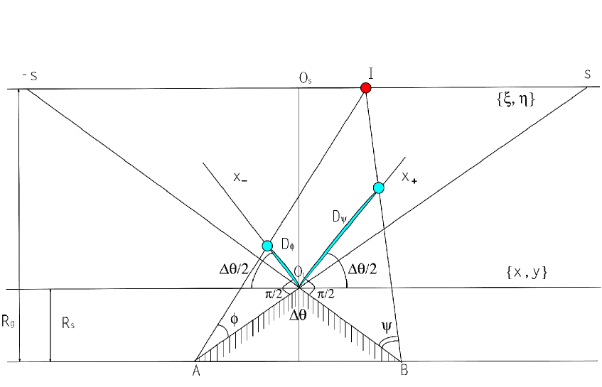
Figure 1: The simplest geometric interpretation of gravitational lensing if a background point-like object (I) is lensed by a cosmic string. The dashed region marks the cut associated to a conical space time once it it is seen in an euclidean space, and the points A and B mark the apparent positions of the observer in the euclidean space. In other words, the observer shall see two images (blue circles) separated by the distance $D=D_{\phi}+D_{\psi}$. For the other symbols, see the text.

In usual gravitational lens theory the main axis coincides with the line joining the observer and the barycenter of the lens. In our case the lens is a one dimensional object, and therefore we may define (see Fig. 1) it as the shortest line which connects the observer and the string. Let now us extend this line to a background object and introduce three planes perpendicular to such main axis The first one is the ”object plane” which intersects the center of the background source; the second one is the ”lens plane” which contains the nearest point of the string, and, finally, the last one, the ”observer plane”, which contains the observer.

Let the background source be point-like. With reference to Fig. 1, axes $O_{S}\xi,O_{S}\eta$ define the coordinate system on the plane of the background source and the origin of this coincides with the intersection of this plane with main axis. The vector $\{\xi,\eta\}$ defines the distance from the origin of object coordinate system to the position of the source $(I)$. The axis $O_{S}\eta$ is perpendicular to the plane of Fig. 1.

On the lens plane we introduce the definition of axes with latin characters. $O_{L}x,O_{L}y$ define the coordinate system in the plane of the string (again, $O_{L}y$ is perpendicular to the plane of Fig. 1) and $x_{-}$ and $x_{+}$ denote respectively the left and right parts of $O_{L}x$ axis the string plane and coincide with the axis $O_{L}x$ when the points A and B are brought together; $\Delta\theta$ is the already introduced deficit angle, $R_{s}$ is the distance between the observer and the string plane, and $R_{g}$ is the distance between the observer and the source. In this geometry and under our assumptions, the observer will see the double images of a background source separated by the angular distance $\delta\theta$:

$$\delta\theta=\Delta\theta{\displaystyle R_{g}-R_{s}\over\displaystyle R_{g}}$$

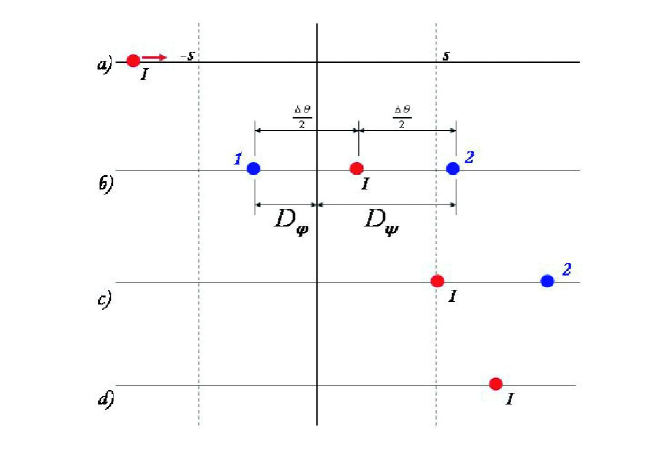
Figure 2: The aspect of the images of a background source as a function of the relative position of the source and of the string strip $[-s,s]$ (done on string plane).

Depending on the position of the background source (Fig. 2) the observer will see one or two images. If the background source $(I)$ falls inside the strip $[-s,s]$, the observer will see two images on the string plane (we wish to stress that, in the euclidean space, this corresponds to the fact that the observer consists of two points A and B).

The lensing equation relates the physical distances (positions on the lens plane) $D_{\phi}$, $D_{\psi}$ with $\xi_{s},\eta_{s}$ (positions on the source plane), as function of the deficit angle $\Delta\theta$, $R_{g}$ and $R_{s}$. Being the deficit angle very small, it is possible to derive a simple relation between angles:

$$\phi+\psi\approx\Delta\theta\biggl{(}1-\frac{R_{s}}{R_{g}}\biggr{)}$$

The angles $\phi$ and $\psi$ are defined as:

$$\psi=\frac{1}{2}\biggl{(}\frac{2\xi_{s}}{R_{g}}+\Delta\theta\frac{R_{g}-R_{s}}{R_{g}}\biggr{)}$$

$$\phi=\frac{1}{2}\biggl{(}-\frac{2\xi_{s}}{R_{g}}+\Delta\theta\frac{R_{g}-R_{s}}{R_{g}}\biggr{)}$$

and:

$$s=\Delta\theta(R_{g}-R_{s})$$

If we omit the second order term, the physical distances $D_{\phi}$, $D_{\psi}$ can be written as:

$$D_{\psi}=R_{s}\psi\mbox{\hskip 56.9055pt}D_{\phi}=R_{s}\phi$$

The lens equation can then be derived from the following equations:

$$x_{1}={\displaystyle R_{s}\over\displaystyle R_{g}}\bigl{(}\xi_{s}+\frac{s}{2}\bigr{)}\mbox{\hskip 56.9055pt}y_{1}={\displaystyle R_{s}\over\displaystyle R_{g}}\eta_{s}$$ (1)

$$x_{2}={\displaystyle R_{s}\over\displaystyle R_{g}}\bigl{(}\xi_{s}-\frac{s}{2}\bigr{)}\mbox{\hskip 56.9055pt}y_{2}={\displaystyle R_{s}\over\displaystyle R_{g}}\eta_{s}$$ (2)

where $x_{1},y_{1}$ and $x_{2},y_{2}$ are the coordinates on the lens plane of the first and second images, respectively.

Therefore, in the case of a point source falling inside the string strip, the observer will observe two identical images of the source, with positions defined by the string lens equations (1 - 2) and, as long as the source is point–like and the photon beams move in a quasi Euclidean space, the two images will have identical optical properties.

2.2 The case of an extended source

The width of a cosmic string strip, defined by its deficit angle, depends on the string linear density (or tension) $\mu$. However the width of the cosmic string itself (or its cross section) is negligible small ($10^{-17}\div 10^{-33}$ cm) being compared with the size of any astronomical object, because its mass scale is not less then 1 TeV.

Thus the size of any extragalactic source is much larger than the width of the string, and any source can be regarded as extended in comparison with the string size. In this case, the general equation of mapping by a string is given by $I(x,y)=$:

$$I({\displaystyle R_{s}\over\displaystyle R_{g}}\bigl{(}\xi_{s}+s/2\bigr{)},{\displaystyle R_{s}\over\displaystyle R_{g}}\eta_{s}) s<\xi_{s}$$

$$I({\displaystyle R_{s}\over\displaystyle R_{g}}\bigl{(}\xi_{s}+s/2\bigr{)},{\displaystyle R_{s}\over\displaystyle R_{g}}\eta_{s})+I({\displaystyle R_{s}\over\displaystyle R_{g}}\bigl{(}\xi_{s}-s/2\bigr{)},{\displaystyle R_{s}\over\displaystyle R_{g}}\eta_{s}) -s\leq\xi_{s}\leq s$$ for

$$I({\displaystyle R_{s}\over\displaystyle R_{g}}\bigl{(}\xi_{s}-s/2\bigr{)},{\displaystyle R_{s}\over\displaystyle R_{g}}\eta_{s}) \xi_{s}<-s$$

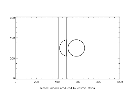
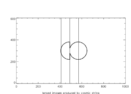
Figure 3: Left: the images of a circular source lensed by a cosmic string. The straight solid line represent the position of the string, while the dashed lines show the position of string strips relative to string itself. Right: the images of a circular source lensed by a cosmic string. The position of string and Einstein strips are the same as in previous figure. The only difference is that the radius of the source is larger than the angular distance between source center and string.

For each point of the source we can follow the same procedure described in the previous paragraph and, if the point is inside the string strip, it will be displayed on the other side of the string, while, if it is not, it will be cut away thus producing sharp edges in the isophotes of the source images. Fig. 3 shows an example of what would happen to a circular source lensed by a string. Notice that the sharp edge introduced by the string is clearly visible. In order to better quantify such effect, let us assume an homogeneous brightness distribution over the disk of the source. It is worth to stress that this assumption does not affect much the generality of the results, since in the case of a source with a radial dependence of the brightness distribution, the source can be approximated as a combination of rings of different brightness and the result can be obtained by integrating over the rings.

Let now the axis of the coordinate system be oriented along the string ($Oy$) and perpendicularly ($Ox$) to it ($O_{L}\equiv O$). The source coordinates will map onto the lens plane in the same way: $\xi$ will coincide with $Ox$, and $\eta$ with $Oy$. It is useful to note explicitly that the origin of the source coordinate system will map into the origin of the lens coordinate system $(\xi=0,\eta=0)\ \rightarrow\ (x=0,y=0)$.

Suppose also that the source has circular shape with radius $\rho_{s}$ and center in $(\xi_{s},\eta_{s})$. The outer contour is then described by the equation:

$$(\xi-\xi_{s})^{2}+(\eta-\eta_{s})^{2}=\rho_{s}^{2}$$ (3)

and the center of the circle will map into:

$$x_{1s}={\displaystyle R_{s}\over\displaystyle R_{g}}\bigl{(}\xi_{s}+\frac{s}{2}\bigr{)}\mbox{\hskip 56.9055pt}y_{1s}={\displaystyle R_{s}\over\displaystyle R_{g}}\eta_{s}$$ (4)

$$x_{2s}={\displaystyle R_{s}\over\displaystyle R_{g}}\bigl{(}\xi_{s}-\frac{s}{2}\bigr{)}\mbox{\hskip 56.9055pt}y_{2s}={\displaystyle R_{s}\over\displaystyle R_{g}}\eta_{s}$$ (5)

where $1$ and $2$ refer, respectively, to the first and second image. The radius in the lens plane becomes:

$r_{i}={\displaystyle R_{s}\over\displaystyle R_{g}}\rho_{s}$

and the outer boundary is described by the equations

$$(x-{\displaystyle R_{s}\over\displaystyle R_{g}}\bigl{(}\xi_{s}\pm\frac{s}{2}\bigr{)})^{2}+(\eta-{\displaystyle R_{s}\over\displaystyle R_{g}}\eta_{s})^{2}=r_{i}^{2}$$ (6)

where the sign differentiates between the first ($+$) and the second ($-$) image.

In fact, an observer does not know the true position of the source in the sky. It can be reconstructed in most cases, but in some cases the reconstruction is not unique. In the simple case when the radius of a source is less then the angular distance between the source center and the string we will define as first image the complete one, while the second will be the incomplete one, as one can see in Fig. 3.

The situation becomes more difficult if the radius of the source (or radius of a ring of the source) becomes larger than the distance between source center and the string.

If part of the first image intersects the string position, all points at $x<0$ (if they obey the eq. (6)) need to be cut away and the corresponding part of circle turns into a straight line coinciding with the string position.

The same is also true for the second image, but inverted: the visible part being that for which $x<0$. In other words, all points obeying eq. (6) and for which $x\leq 0$, need to be cut out and replaced with a straight line coinciding with the string position. The edge in the first image appears if the radius of the circle is larger than $\rho_{s}>\eta_{s}+s$ (see Fig. 3, right panel). We shall therefore assume $\eta_{s}>0$.

The linear size of the edge can be written as:

$$\Delta y_{1}=2{\displaystyle R_{s}\over\displaystyle R_{g}}\sqrt{\rho_{s}^{2}-\bigl{(}\eta_{s}+s\bigr{)}^{2}}$$

When the edge is absent, the total flux from the source is proportional to the source area $\sim\pi\rho_{s}^{2}$.

In the opposite case, the total area is smaller and becomes:

$$A_{1}=\bigl{(}\pi-\phi_{1}+\frac{1}{2}\sin 2\phi_{1}\bigr{)}\rho_{s}^{2}$$

where:

$\sin\phi_{1}={\displaystyle\Delta y_{1}\over\displaystyle 2r_{s}}.$

Also for the second image the edge is defined by the condition $x=0$, and the size of the edge is given by:

$$\Delta y_{2}=2{\displaystyle R_{s}\over\displaystyle R_{g}}\sqrt{\rho_{s}^{2}-\bigl{(}\eta_{s}-s\bigr{)}^{2}}$$

The condition $\rho_{s}\leq|\eta_{s}-s|$ must then be matched in order to produce the edge in the second image. This inequality is not uniquely defined. In fact, if the center of the source falls outside the Einstein strip ($\eta_{s}>s$), the center of the second image is to the right hand side of the string, and an observer sees less then half of the circle (case A). If the center of the source is inside the Einstein strip ($\eta_{s}<s$), then the center of the second image is on the left hand side of the string, and an observer sees more than half of the circle (case B). In both cases the sizes of the edges are equal.

In case A, the visible area is equal to:

$$A_{1A}=\bigl{(}\phi_{2}-\frac{1}{2}\sin 2\phi_{2}\bigr{)}\rho_{s}^{2}$$

where

$\sin\phi_{2}={\displaystyle\Delta y_{2}\over\displaystyle 2r_{s}}.$

Instead, in case B, the visible area is equal to:

$$A_{2B}=\bigl{(}\pi-\phi_{2}+\frac{1}{2}\sin 2\phi_{2}\bigr{)}\rho_{s}^{2}$$

If the first image does not produces an edge, while the second one does (see for instance Fig. 3), the size of the edge will be equal to that in the second image. If, instead, the edge in the first image does exist, the total size of the edge will be equal to the difference between the edges in the first and second image (see Fig. 3, right panel). This remark is crucial to understand ground based observations. In fact, in this case we need to probe very low surface brightness isophotes in order to detect the edge.

Furthermore, since these isophotes will usually have large radii, the edges in the two images will merge and the resulting appearance will be given by the difference between the two edges.

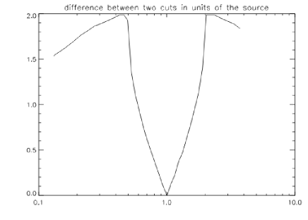
Figure 4: Graph showing the difference between two edges (edge of first and second images) as function of images intensities. The difference value is plotted along vertical axes. The ratio of intensities of two images is plotted along the horizontal axes and the scale is logarithmic

Fig. 4 shows the difference between the two edges as a function of the intensity ratio of the two images ($F$). One can see that $F=1$ corresponds to zero difference. Generally speaking the case where the value of $F$ is around unity is very hard to disentangle (especially in presence of noise) from that of a chance alignment of two similar looking galaxies.

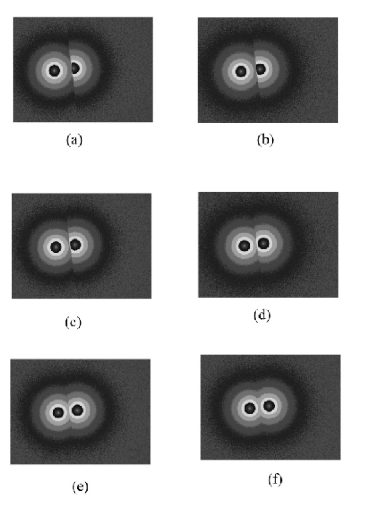
Figure 5: The images of a source lensed by a cosmic string. We assume de Vaucouleurs profile brightness distribution over disk. Each picture represent one step relative to position of the string. Noise is included (see text).

Fig. 5 presents the effects produced by a typical string (whith mass scale of the order of $10^{15}$ GeV) upon a background galaxy at redshift z$\sim$ 0.5, producing splitted images $\sim 2$ arcsec apart.

If the ratio falls within the $0.9<F<1.1$ range, the difference between the edges is smaller than 0.1 of the source radius ($\leq$ 0.2 arcsec in our case) and therefore very high angular resolution is required in order to detect it. The difference increases when the ratio $F$ increases (or decreases) and, for instance, when it is $\sim 2$, the difference is almost equal to the radius size. The above discussion confirms that the detection of sharp edges of pairs of lensed images along the position of the string is, at least in theory, possible also from the ground.

We wish also to stress that one of the most characteristic features of lensing by a cosmic string is the fact that all details (such as galactic arms, bright spots, globular clusters, supernovae, etc.) which are present in the first image, will also be reproduced in the second one if they fall inside the string strip.

An additional feature appears if we take into account the possible time delay between two images, which is determined by the difference between the two photon paths (AI and BI, see Fig. 1).

$$BI=\frac{R_{g}}{\cos{(\Delta\theta/2-\psi)}},$$

$$AI=\frac{R_{g}}{\cos{(\Delta\theta/2-\phi)}}.$$

and the difference between the two paths can be written as:

$$\Delta L={\displaystyle 1\over\displaystyle 2}R_{s}\Delta\theta(\psi-\phi)$$ (7)

where $\Delta L=AI-BI$. This difference can also be written in terms of the coordinates in the source plane:

$$\Delta L={\displaystyle R_{s}\over\displaystyle R_{g}}\xi_{s}\Delta\theta$$

The best way to represent this value is in observable terms. In eq. (7) only one term $R_{s}$ has to be expressed in terms of $\sim H^{-1}$ to get the time delay expressed in observable values:

$$\Delta t={\displaystyle 1\over\displaystyle 2H}f(z_{s},\Omega_{m},\Omega_{\Lambda})\Delta\theta(\psi-\phi)$$

where $H$ is the Hubble parameter, $z_{s}$ is the redshift of string, $\Omega_{m},\Omega_{\Lambda}$ are the contributions of matter and dark energy respectively, and $f$ is a function which describes the cosmic distance to the string.

When dealing with time delays, a possible source of misinterpretation could be the presence of a variable object within the source. In the case of a supernova, for instance, the time delay between the two images would become important since, should it be greater than the characteristic variability time of supernovae, it could be seen in one image and not in the other.

3 Simulated images produced by a cosmic string.

In order to produce realistic simulations of the effect described above, we made use of a ”virtual” galaxy obtained using a de Vaucouleurs surface brightness profile (de Vaucouleurs, 1953):

$$I(r)=I_{v}exp(-7.6692({\displaystyle r\over\displaystyle r_{ch}})^{1/4})$$

truncated at $r>10r_{e}$ in order to speed up computations. To be as realistic as possible, we used the redshift, apparent magnitude in the Johnson $V$ band and effective radius derived for CSL-1 in Sazhin et al. (2005) which are equal to $z=0.46$, $V=21.05$ and $r_{e}=1.6"$, respectively. As observational parameters we assumed those adopted in our HST observations of CSL-1 (which are rather typical). We assumed a pixel size of 25 mas, i.e the pixel size achievable with HST and typical dithering, and convolved the model with a FWHM=0.1” PSF to simulate the angular resolution expected in the F814 band (which roughly corresponds to the rest-frame V band). We used a stochastic process to compute the Poissonian noise per pixel, using the expresion:

$$\sqrt{(C+B_{sky}+B_{det})t+n_{read}N^{2}}$$ (8)

where $t=14$ ks is the total exposure time, $C$ is the signal from the astronomical source in counts/second, $B_{sky}$ and $B_{det}$ are the average sky and detector background, $N$ is the readout noise and $n_{read}$ is the number of CCD readouts. The actual values of $B_{sky}$, $B_{det}$ and $N$ were obtained from the ACS Instrument Handbook.

Note that when multiple observations are dithered and stacked the actual noise statistics is not simply represented by the expr. (8) due to correlation among pixels on scales given by the dithering pattern (Casertano et al., 2000; Fruchter & Hook, 2002). However for our observations this results in a noise suppression factor of $\sim 2$ which can be compensated by rebinning as long as the lensing signatures are large compared to the pixel scale. Furthermore the comparison of Fig. 5 and 7 shows that expr. (8) is adequate for the simple model discussed here.

The simulated elliptical was then placed within the lensing strip at different angular distances with respect to the string. In Fig. 5 we show the results of our simulations. The figure is composed by 6 panels (a through f) corresponding to intensity ratios $F$ equal to $1.4$, $1.27$, $1.18$, $1.10$, $1.04$, and $0.99$, respectively. The latter value corresponds to an almost symmetric situation, in which the observer will hardly see the sharp edges produced by the string even with high (HST like) angular resolution.

We notice that in the case of CSL-1 the intensity ratio of the two components falls in the range $1.06-1.04$ and therefore roughly corresponds to panel (e). In the images, the sharp ”edges” introduced in the outer isophotes by the string are apparent.

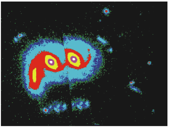
a)

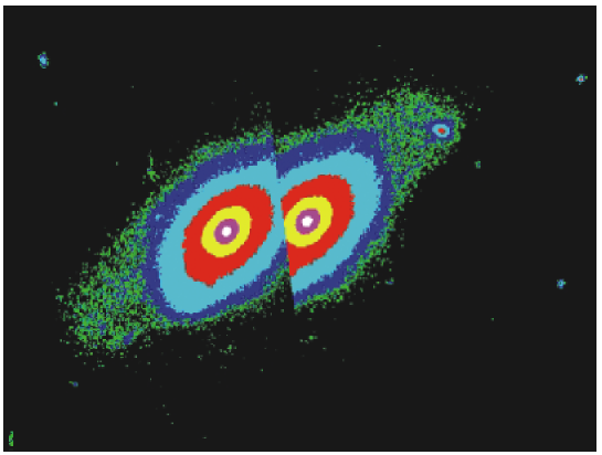
b)

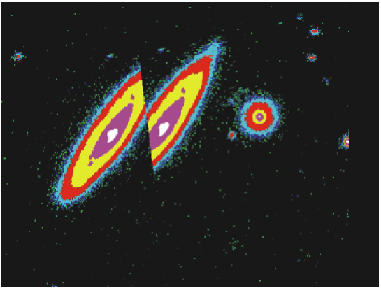
c)

Figure 6: Panel a: this picture represent the lensed image of a spiral galaxy. The direction of a string is almost perpendicular to galaxy plane. Duplicated details are clearly visible. Panel (b): in this case, the string is inclined with respect to the galaxy plane. As a result sharp edge appears. Panel (c): Also in thei case the direction of string is inclined with respect to galactic plane.

For completeness, we also present the lensed images of a set of three spiral galaxies extracted from our HST data (Fig. 6).

4 HST image of CSL-1.

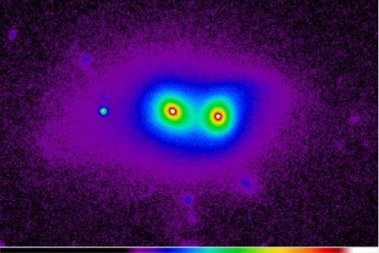
Figure 7: CSL-1 image in pseudocolor as obtained by stacking (see text) 6 HST orbits obtained on January 11, 2006 in the F814W band.

To test whether CSL-1 was actually a lens produced by a cosmic string we observed the double source with the HST/ACS camera during Cycle 14, using Director’s Discretionary Time. CSL-1 was observed for 6 HST orbit in the F814W band (comparable to Johnson-Cousins I-band) yielding an effective exposure time of $\sim 14000$ seconds. The observations were performed adopting a 1/3 pixel dither pattern, to allow sub-pixel sampling of the HST PSF and accurate cosmic ray rejection. All 6 orbits were combined through the Multidrizzle software Koekemoer et al. (2002) using a 1/2 pixel (0.025 arcsec/pixel) resampling pattern. In Fig. 7 we show the final stacked image.

As it can be seen by comparison with our simulations (panel (e) of Fig. 5) in the HST data there is no sign of the peculiar features (sharp edges) predicted in the case of lensing by a cosmic string. The faint isophotes of the two components have different shapes, which is incompatible with CSL-1 being lensed by a cosmic string. In fact in the cosmic string scenario all morphological features of the source falling inside the deficit angle, would be mirrored on the opposite side of the string. However in the HST image we do not see such mirroring effect for the two components, nor for any other faint feature which, would have fallen inside the deficit angle of the string and should have been duplicated, e.g. the faint sources on the southern side of CSL-1 visible in the right panel of Fig. 7.

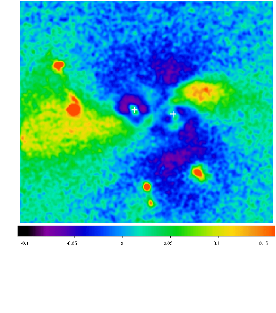
Figure 8: The normalized residuals (residuals/model) obtained by subtracting from the HST images a model consisting of two de Vaucouleurs light profiles. Crosses mark the centroids of the two galaxies.

To further check whether the distortions observed in the faint isophotes are caused by tidal interactions between the two ellipticals we fit the two objects with two de Vaucouleurs $r^{1/4}$ light profiles and subtract the model from the original data. The residual image, presented in Fig.8, clearly shows the presence of warped structures in the CSL-1 outskirts, most probably tidal tails due to the interaction between the two galaxies. The detailed photometry of the objects will be discussed elsewhere (Paolillo et al. in preparation).

5 How many lensing pairs we have to expect?

As discussed in Sec.1, the most evident signature of a cosmic string is to produce a strip of multiple images along its path. This would be the first feature to look for in any dedicated search for cosmic strings within large astronomical surveys. As template cases, in what follows we derive the expected number of lensed images using as template case the CSL-1 field as it appears in the $R$ band mosaic taken from the OAC - Deep Field (OACDF) (Capaccioli et al., 2002; Alcalá et al., 2004) and in the deeper observations obtained with HST.

The presence of a background galaxy inside the deficit angle of a string is a stochastic process determined by the area of the lensing strip and by the density (number of objects per unit solid angle) of background galaxies. The larger is the field of search, the larger is the number of lensed objects that should be found.

All lensed objects will fall inside the narrow strip defined by the path of the string and by the deficit angle. Along this path, an observer should therefore see a sort of ”milky way” of double images of galaxies. Historically speaking, this effect was first discussed by Vilenkin (1981, 1984, 1986); Hindmarsh (1990); Huterer & Vachaspati (2003), and we shall just summarize it briefly in the framework of a simple model. For the sake of simplicity, we shall consider all background object as point–like sources. In the case of a straight string, one can easily estimate the expected number of lensed galaxies as

$$\left<N\right>=n_{g}2l\Delta\theta$$ (9)

Here $n_{g}$ is the density of galaxies per unit solid angle, $\Delta\theta$ is the deficit angle of the string, and $l$ is the length of the string in the chosen field. Both $\Delta\theta$ and $l$ are expressed as angular measures. A more complex case emerges if the string is assumed to be curved Huterer & Vachaspati (2003). A simple estimate can be derived as it follows. The lenght of a curved string is larger than that of a straight one; therefore, the lensing strip will cover a larger area on the sky in the same patch and its lenght can be written as (Huterer & Vachaspati, 2003):

$$l=\varrho\left(\frac{\varrho}{l_{c}}\right)^{a}$$

Here $\varrho=|\vec{r}-\vec{r}_{1}|$ is the distance from the point $\vec{r}$ to the point $\vec{r}_{1}$. $l_{c}$ is the correlation interval. The parameter $a$ varies between $0$ (straight string) and $1$ (in the case of random walk of the string); the last value corresponding to purely brownian motion ($\varrho\sim\sqrt{l}$).

In the case ($a=1$), the expected number of lenses is:

$$\left<N\right>=2\frac{\Delta\theta}{l_{c}}n_{g}A$$

where the product of the angular area $A$ of the patch times the surface density of galaxies $n_{g}$ gives the number of galaxies expected in the patch. Therefore, in the case of a straight string, the minimum number of lensed objects is proportional to the number of galaxies falling inside the string strip.

In order to to estimate such figures, and compare them with what is actually observed in the CSL-1 field, we must derive the number of galaxies brighter than the assumed limiting magnitude in the $R$ and F814W band.

Counts in the $R$ band can be obtained from the existing literature, such as the moderately deep data by Kummel & Wagner (2001). Deeper counts were obtained (cf. Gardner et al., 1996) at slightly different wavelength, and they need therefore to be interpolated. Additional information, for the F814W filter can be found in Thomson et al. (1999), Gardner (1998), Shanks et al., (1998), Gardner and Satyapal (2000), based on the Hubble Deep Field. Using the Kummel & Wagner (2001) counts and extrapolating them to $m=24$ in the $R$ band, we derive that in the OAC-DF, in a field of 16′$\times$16′, there should be $\sim 2200$ galaxies having magnitudes in the range $20<m_{R}<24$. Comfortably enough, this figure matches the number of extended sources actually detected in the OAC-DF.

Using the above estimate, in the case of a straight string we expect at least 9 lenses, while in the case of a random walk string, the expected number is much larger: $\sim 200$. Obviously, in the same region of the sky, also lenses produced by galaxies or conventional lenses should be present, and their average density can be derived through the product of the optical depth due to lensing, times the number of galaxies in the field (Fukugita et al., 1992; Kochanek, 1993; Chiba & Yoshi, 1999; Ofek et al., 2003, cf.). These estimates lead to an expected number of $\sim 2$ conventional lenses within the same magnitude range as above and within the same area.

In the case of HST observation the number of lensed pairs should decrease due to the smaller field of view and increase due to the fainter limiting magnitude ($\sim 28$ in the F814W band and for point like sources). For limiting magnitude the signal to noise ratio is equal to 9 roughly. In this case the number of galaxies per unit of solid angle is (Williams et al. (1996)): is $n\approx 10^{6}deg^{-2}$ for magnitude $AB\leq 28$.

The field of view of the ACS/WFC on HST is roughly 3.5′$\times$ 3.5′, so that the maximum length, for a straight strip crossing diagonally the FOV, is $\sim 5\ arcmin$. Assuming that the width of the string strip is $\sim 2\ arcsec$ as we already discussed above, eq. (9) gives an average number of $\sim 40$ lensed pairs within the HST field. The HST image of the CSL-1 field in Sazhin et al. (2006) shows no trace of an excess of galaxy pairs, further ruling out the existence of a cosmic string in the field.

6 Conclusions

In the present work, we presented a detailed analysis of the observable effects induced by the gravitational field of a cosmic string and tested it against our recent HST observations of the lens candidate CSL-1.

Our observations proved, beyond any doubts, that CSL-1 is a rather peculiar pair of interacting ellipticals and its detailed photometry will be presented elsewhere (Paolillo et al in preparation). The results of our analysis lead to some general conclusions which will be useful in future searches for possible gravitational signatures of cosmic strings to be performed in existing or future digital surveys.

It is likely (Allen & Shellard, 1990; Polchinski and Rocha, 2006) there are a few dozen long strings crossing horizon volume and therefore, any survey aimed at detecting them through the photometric signature induced by the gravitational lensing phenomenon needs to be multiband, very deep and of high photometric accuracy. Our simulations showed that, while high angular resolution (HST like) is not required to produce lists of candidates, it is definitely needed in order to disentangle whether these candidates actually are the signatures of a string and to constrain the physical properties of the string.

References

- Agol et al. (2006) Agol, E., Hogan, C. J., & Plotkin, R. M. 2006, Phys.Rev. D, 73, 087302
- Alcalá et al. (2004) Alcalá J.M., et al., 2004, A&A, 428, 339
- Allen & Shellard (1990) Allen B. and Shellard E.P.S., 1990, Phys.Rev.Lett., 64, 119.
- Bennett & Bouchet (1990) Bennett, D. P., & Bouchet, F. R. 1990, Phys.Rev. D, 41, 2408
- Bernardeau & Uzan (2000) Bernardeau F., Uzan J.-P., 2001, Phys.Rev D, 63, 023004, 023005
- Bevis et al. (2004) Bevis, N., Hindmarsh, M., & Kunz, M. 2004, Phys.Rev. D, 70, 043508
- Bevis et al. (2006) Bevis N., Hindmarsh M., Kunz M., & Urrestilla J., 2006, astro-ph/0605018.
- Capaccioli et al. (2002) Capaccioli M., Alcalá J.M., Radovich M., Silvotti R., Ortiz P.F., et al., 2002, Proc. SPIE 4836, pp.
- Carretero et al. (2006) Carretero et al. 2006, astro-ph/0608012
- Casertano et al. (2000) Casertano, S., et al., 2000, AJ, 120, 2747
- Chiba & Yoshi (1999) Chiba M., Yoshi Yu., 1999, Ap.J., 510, 42
- Copeland et al. (2004) Copeland E.J., Myers R.C., Polchinski J., 2004, JHEP, 06:013.
- Davis & Kibble (2005) Davis A.-C., Kibble T.W.B., 2005, hep-th/0505050
- Damour and Vilenkin (2004) Damour T. and Vilenkin A., hep-th/0410222.
- Fruchter & Hook (2002) Fruchter, A. S., & Hook, R. N., 2002, PASP, 114, 144
- Fukugita et al. (1992) Fukugita, M., Futamase, T., Kasai., Turner E.L., 1992, Ap.J., 393, 3
- Gardner et al. (1996) Gardner J.P., Sharples R.M., Carraso B.E., Frenk C.S., 1996, MNRAS, 282, L1
- Gardner (1998) Gardner J., 1998, PASP, 110, 291
- de Vaucouleurs (1953) de Vaucouleurs, G. 1953, MNRAS, 113, 134
- Shanks et al., (1998) Shanks T., Metcalfe N., Fong R., et al., 1998, in: The Young Universe, ASP Conference Ser., Eds. S.D’Odorico, A.Fontana, E.Gialongo, v.146, p.102.
- Gardner and Satyapal (2000) Gardner J., Satyapal S., Astron.J., 2000, 119, 2589
- Hindmarsh (1990) Hindmarsh. A.,in ”The Formation and Evolution of Cosmic Strings”, ed. G.Gibbons, S.W.Hawking & T.Vachaspathi. Cambridge Univ.Press., Cambridge, 1990.
- Huterer & Vachaspati (2003) Huterer, D., Vachaspati, T., 2003, preprint. astro-ph/0305006.
- Kibble (1976) Kibble T.W.B., 1976, J.Phys.A:Math & Gen. v.9, 1387
- Kochanek (2002) Kochanek et al., 2002, http://cfa-www.harvard.edu/castles/
- Kochanek (1993) Kochanek C.S., 1993, MNRAS, 261, 453
- Koekemoer et al. (2002) Koekemoer, A.M., Fruchter, A.S., Hook, R., Hack, W. 2002 HST Calibration Workshop, 337.
- Kummel & Wagner (2001) Kummel M.W., Wagner S.J., 2001, astro-ph/0102036.
- Laix & Vachaspati (1996) de Laix, A.A., Vachaspati, T., 1996, Phys.Rev. D 54, 4780, 1996.
- Majumdar (2005) Majumdar M., hep-th/0512065.
- Ofek et al. (2003) Ofek E.O., Rix H-W., Maoz D., 2003, MNRAS, 343, 639
- Polchinski and Rocha (2006) Polchinski, J. & Rocha, J.V., hep-ph/0606205
- Ringeval et al. (2005) Ringeval C., Sakellariadou M. & Bouchet F., 2005, astro-ph/0511646.
- Sazhin et al. (2003) Sazhin, M., et al., 2003, MNRAS, 343, 353
- Sazhin et al. (2005) Sazhin, M., Capaccioli, M., Longo, G., Paolillo, M., & Khovanskaya, O. 2006, ApJ, 636, L5
- Sazhin et al. (2006) Sazhin, M., et al., 2006, astro-ph/0601494
- Schneider, Ehlers, Falco (1992) Schneider P., Ehlers J., Falco E.E., 1992, Gravitational Lenses, Springer, Heidelberg.
- Shirasaki, Mizumoto, Ohishi (2004) Shirasaki, Y., Mizumoto, Y., Ohishi, M. et al. ASP Conference Series, vol. 314, 2004.
- Shlaer and Tye (2005) Shlaer B., Tye S.-H. Henry, hep-th/0502242.
- Thomson et al. (1999) Thomson, R.I., Storrie -Lombardi, L.J., Weymann, R., et al., 1999, Astron.J., 117, 17.
- Tye et al. (2005) Tye S.-H.Henry, Wasserman Ira and Mark Wyman, astr-ph/0503506.
- Vilenkin (1981) Vilenkin A., 1981, Phys.Rev. D, 23, 852
- Vilenkin (1984) Vilenkin A., 1984, ApJ, 289, L51.
- Vilenkin (1986) Vilenkin A., 1986, Nature, 322, 613.
- Vilenkin, Shellard (1994) Vilenkin A., Shellard E.P.S, 1994, Cosmic strings and other topological defects. Cambridge Univ.Press., Cambridge.
- Vincent et al. (1998) Vincent, G., Antunes, N. D., & Hindmarsh, M. 1998, Phys. Rev. Letters, 80, 2277
- Williams et al. (1996) Williams, R. E.; Blacker, B.; Dickinson, M. Astron.J., 1996, v.112, p.1335.
- Zakharov and Sazhin (1998) Zakharov A.F., Sazhin, M.V., 1998, PHYS-USP, 41(10), 945.
- Zeldovich (1980) Zeldovich, Ya.B., 1980, MNRAS, 192, 663
a)
a)
b)
b)
c)
c)