The circumburst environment of a FRED GRB: study of the prompt emission and X-ray/optical afterglow of GRB 051111

Abstract

Aims. We report a multi-wavelength analysis of the prompt emission and early afterglow of GRB 051111 and discuss its properties in the context of current fireball models.

Methods. The detection of GRB 051111 by the Burst Alert Telescope on-board Swift triggered early BVRi’ observations with the 2-m robotic Faulkes Telescope North in Hawaii, as well as X-ray observations with the Swift X-Ray Telescope.

Results. The prompt $\gamma$-ray emission shows a classical FRED profile. The optical afterglow light curves are fitted with a broken power law, with ${\alpha}_{1}=0.35$ to ${\alpha}_{2}=1.35$ and a break time around 12 minutes after the GRB. Although contemporaneous X-ray observations were not taken, a power law connection between the $\gamma$-ray tail of the FRED temporal profile and the late XRT flux decay is feasible. Alternatively, if the X-ray afterglow tracks the optical decay, this would represent one of the first GRBs for which the canonical steep-shallow-normal decay typical of early X-ray afterglows has been monitored optically. We present a detailed analysis of the intrinsic extinction, elemental abundances and spectral energy distribution. From the absorption measured in the low X-ray band we find possible evidence for an overabundance of some $\alpha$ elements such as oxygen, [O/Zn]=$0.7\pm 0.3$, or, alternatively, for a significant presence of molecular gas. The IR-to-X-ray Spectral Energy Distribution measured at 80 minutes after the burst is consistent with the cooling break lying between the optical and X-ray bands. Extensive modelling of the intrinsic extinction suggests dust with big grains or grey extinction profiles. The early optical break is due either to an energy injection episode or, less probably, to a stratified wind environment for the circumburst medium.

1 Introduction

The launch of the the Swift satellite in November 2004 (Gehrels et al. Gehrels04 (2004)) ushered in a new era of rapid detection, accurate localisation and observation of prompt $\gamma$-ray emission early X-ray afterglows of Gamma-Ray Bursts (GRBs). Thus for the first time, it became possible to explore the previously unknown behaviour of the early X-ray afterglow from seconds to hours after the burst with unprecedented sensitivity, as well as to trigger rapid GRB followup observations from ground-based facilities working across the electromagnetic spectrum. As a result, there is an increasing number of GRBs with good early-time optical and X-ray coverage. Early multi-band observations are crucial to discriminate between several models; for example, the discovery that X-ray afterglow light curves can exhibit a variety of complex properties such as flares and steep early decays, has driven modifications to the standard fireball model with late central engine activity suggested to explain flares and continuous energy injection to account for the observed intermediate shallow decay phase (e.g. Chincarini et al. Chincarini05 (2005); Nousek et al. Nousek06 (2006)).

In addition, the combination of early optical and X-ray data sheds light on the circumburst environment properties. In particular, the presence of dust and its properties with respect to gas can be studied through the optical extinction vs. X-ray absorption. In this regard, in a seminal paper Galama & Wijers (Galama01 (2001)) found that the optical extinction is lower than expected from the X-ray absorption measured in terms of equivalent hydrogen column density; see also the comprehensive studies by Stratta et al. (Stratta04 (2004)) and Kann et al. (Kann06 (2006)). For a number of GRBs at high redshift ($z\gtrsim 4$) for which an optical spectrum is available, a damped Lyman $\alpha$ absorption feature was observed. These systems are called GRB Damped Lyman Systems (GRB-DLAs) in analogy to the QSO-DLAs (Wolfe et al. Wolfe05 (2005)); see Savaglio (Savaglio06 (2006)) for an updated review of the properties of both classes. The properties that characterise the GRB-DLAs appear to be peculiar and suggest a different ISM in the GRB hosts compared to that of the Milky Way or Magellanic clouds, particularly for those GRBs at high redshift. These peculiarities could be ascribed to either the circumburst environment or to the GRB host itself, or to the combination of the two.

A possible connection has been suggested between GRBs whose $\gamma$-ray temporal profiles exhibit few pulses and the nature of the progenitor as a SN (Bosnjak et al. Bosnjak06 (2006), Hakkila & Giblin Hakkila06 (2006)). Despite the variety of temporal profiles of GRBs, the so-called FRED GRBs (“Fast Rise Exponential Decay”) seem to identify a subclass of GRBs (Fishman et al. Fishman95 (1995)). The multi-wavelength study of the early afterglow of this kind of GRBs can be a further way to test this connection, providing possible keys to the understanding of the variety of the prompt light curves, still so poorly understood.

In this paper, we report the robotic detection and automatic identification of the optical afterglow of a classical FRED detected by Swift, GRB 051111, using the 2-m Faulkes Telescope North (FTN) located in Maui, Hawaii, from 3.9 to 168 minutes after the GRB trigger time. We also report the Swift/BAT and XRT observations of the prompt $\gamma$-ray event and of the X-ray afterglow, respectively. The redshift of this burst is known spectroscopically: $z=1.55$ (Hill et al. Hill05 (2005)). The paper is structured as follows. In Sec. 2 observations are reported. The results are presented in Sec. 3. In Sec. 4 we discuss the Spectral Energy Distribution (SED) at $t=80$ minutes after the burst, when we have the best clustering of observations from IR to X-rays. In particular, we derive clues on the circumburst environment properties by comparing the intrinsic optical extinction and the X-ray absorption. In Sec. 5 we discuss some possible interpretations of the overall picture.

2 Observations

2.1 Swift/BAT Observations

On 2005 November 11 at 05:59:41 UT GRB 051111 triggered Swift/BAT, which automatically on board provided the location of the burst with an error radius of 3 arcmin (90% CL; Sakamoto et al. Sakamoto05 (2005)). During the prompt event, the spacecraft did not slew because of the angular proximity of the GRB to the Moon. Data have been reduced following the standard BAT pipeline (Krimm et al. Krimm04 (2004)) with the HEASARC heasoft package (v. 6.0.4): we created a detector plane image and a merged quality mask and finally we added a mask weight column to the event file using the direction of the burst (see Section 2.3). Mask-weighted light curves and time-resolved spectra were extracted. Spectra have been corrected for systematics with the tool batphasyserr as recommended by the BAT team .

2.2 Swift/XRT Observations

XRT began observing the afterglow of GRB 051111 from 95 minutes to about 900 minutes after the burst. We consider here only the data in Photon Counting (PC) mode. Data have been processed following the standard XRT pipeline with the ftool xrtpipeline (v. 0.9.9) using standard screening criteria. We extracted light curves and spectra from a 20-pixel radius circle centred on the optical afterglow. We found that pile up was negligible, following Vaughan et al. (Vaughan06 (2006)). Background was determined from four 50-pixel radius circles with no sources. Spectral analysis was done adopting either empirical and physical ancillary files. We adopted the response function of the latest distribution of the HEASARC calibration database (CALDB 2.3).

2.3 Faulkes Telescope North Observations

The optical afterglow was discovered by the ROTSE-IIIb telescope 27 s after the burst within the BAT error circle and with an unfiltered magnitude of 13.0 (Rujopakarn et al. ROTSE05 (2005)).

The optical afterglow was soon confirmed by the FTN which robotically followed up GRB 051111 at 3.87 min after the burst trigger time (3.5 min after the GRB notice time). The optical transient (OT) candidate was identified automatically and independently of ROTSE-IIIb as a fading uncatalogued source with initial magnitude $R\sim 14.9$ (Mundell et al. Mundell05 (2005)). The automatic identification of the OT with the highest confidence level (1.0) by the GRB pipeline “LT-TRAP” (Guidorzi et al. Guidorzi06 (2006)) triggered a multi-colour imaging sequence: however, after the first 3x10 s $R$ images, followed by 3x10 s in $B$, $V$ and Sloan $i^{\prime}$, the telescope unexpectedly stopped observing due to technical problems. A manual intervention restored the follow-up observation program at $\sim$36 min after the burst. The sequence of filters used reflects the strategy described by Guidorzi et al. (Guidorzi06 (2006)) for the multicolour image mode (MCIM) for the FTN. A late follow-up observation with FTN was performed from 100 to 168 minutes after the burst in the $BVRi^{\prime}$ filters as part of the RoboNet project. Table 1 summarises the observations with FTN.

Table 1: Optical photometry for GRB 051111 with the Faulkes Telescope North

Filter	Starta	Enda	Exp.	Mag.	Commentb
	(min)	(min)	(s)
Bessell-R	3.87	4.04	10	$14.92\pm 0.03$	DM
Bessell-R	4.23	4.40	10	$14.98\pm 0.03$	DM
Bessell-R	4.58	4.75	10	$15.03\pm 0.03$	DM
Bessell-B	5.88	6.05	10	$16.32\pm 0.04$	MCS
Bessell-V	6.72	6.89	10	$15.87\pm 0.03$	MCS
SDSS-I	7.63	7.80	10	$15.30\pm 0.02$	MCS
Bessell-R	36.1	37.0	3x10	$16.99\pm 0.09$	DM
Bessell-B	38.18	38.35	10	$18.20\pm 0.14$	MCS
Bessell-V	39.03	39.20	10	$17.82\pm 0.14$	MCS
SDSS-I	39.95	40.12	10	$17.07\pm 0.07$	MCS
Bessell-B	41.6	42.1	30	$18.30\pm 0.08$	MCS
Bessell-R	42.9	43.4	30	$17.22\pm 0.07$	MCS
SDSS-I	44.2	44.7	30	$17.19\pm 0.04$	MCS
Bessell-B	45.4	46.4	60	$18.48\pm 0.08$	MCS
Bessell-R	47.3	48.3	60	$17.33\pm 0.05$	MCS
SDSS-I	49.1	50.1	60	$17.40\pm 0.03$	MCS
Bessell-B	50.8	52.8	120	$18.41\pm 0.05$	MCS
Bessell-R	53.6	55.6	120	$17.47\pm 0.04$	MCS
SDSS-I	56.3	69.6	120+180	$17.56\pm 0.03$	MCS
Bessell-B	59.1	62.1	180	$18.80\pm 0.05$	MCS
Bessell-R	62.8	65.8	180	$17.79\pm 0.04$	MCS
Bessell-B	70.4	72.4	120	$18.81\pm 0.08$	MCS
Bessell-R	73.2	75.2	120	$17.78\pm 0.05$	MCS
SDSS-I	76.0	89.4	120+180	$17.97\pm 0.04$	MCS
Bessell-R	82.6	85.6	180	$18.13\pm 0.06$	MCS
Bessell-B	90.1	94.1	240	$19.23\pm 0.09$	MCS
Bessell-R	95.0	99.0	240	$18.25\pm 0.06$	MCS
Bessell-R	100.6	108.4	3x150	$18.34\pm 0.06$	LFU
Bessell-R	108.6	111.1	150	$18.44\pm 0.08$	LFU
Bessell-V	112.5	123.1	4x150	$18.95\pm 0.10$	LFU
Bessell-B	124.4	135.0	4x150	$19.75\pm 0.14$	LFU
SDSS-I	157.0	167.5	4x150	$18.66\pm 0.09$	LFU

Magnitudes in $BVR$ have been calibrated using Landolt standard field stars (Landolt Landolt92 (1992)). The zero points derived from observations of standards before and after the GRB observations were consistent. Magnitudes in $i^{\prime}$ have been calibrated using the same Landolt standard field stars, after converting from Bessell $RI$ values to SDSS $r^{\prime}i^{\prime}$ assuming power-law spectra. Magnitudes have been corrected for the airmass and Galactic extinction. The latter was estimated from the $E_{B-V}=0.159$ derived from the extinction maps by Schlegel et al. (Schlegel98 (1998)), and $A_{V}=R_{V}\cdot E_{B-V}=0.49$, with $R_{V}=3.1$. We evaluated the extinction in the other filters following the parametrisation by Cardelli et al. (Cardelli89 (1989)): $A_{B}=0.64$, $A_{R}=0.40$ and $A_{i^{\prime}}=0.32$. Magnitudes have been converted into flux densities $F_{\nu}$ (mJy) following Bessell (Bessell79 (1979)) and Fukugita et al. (Fukugita96 (1996)) for the $BVR$ and $i^{\prime}$ pass-bands, respectively.

3 Results

All the reported parameter uncertainties are given at 1-$\sigma$ confidence level (CL), unless stated otherwise.

3.1 The $\gamma$-ray prompt emission

The 15–150 keV temporal profile is that of a typical FRED and the mask-weighted light curve shows significant emission above the background up to about 90 s after the burst onset time (Fig. 1).

Figure 1: Top Panel: Swift/BAT 15–150 keV mask-weighted light curve of GRB 051111. The burst onset time corresponds to 21573.312 seconds of day (corresponding to 8 s earlier than the trigger time). Bottom Panel: the same light curve in log scale. Dashed line shows the best-fit power-law applied to $t>18\leavevmode\nobreak\ s$ data: $\alpha_{\gamma}=1.8\pm 0.2$ ($F_{\gamma}\sim t^{-\alpha_{\gamma}}$).

The onset of this burst was 8 s before the trigger time, which is 21581.312 SOD UT, and is assumed as zero time hereafter. The spectral evolution is typical, from hard to soft, as shown by the hardness ratio temporal evolution between the 15–50 keV and 50–150 keV (Fig. 2).

Figure 2: Top Panel: BAT light profiles of the mask-weighted light curve in two energy channels: 15–50 keV and 50–150 keV. Bottom Panel: the hardness ratio between the two energy channels exhibits a typical hard-to-soft evolution. The three temporal intervals correspond to the three different energy spectra discussed in the text.

The fit of the $\gamma$-ray tail alone with a power law for $t>18$ s gives an acceptable result, with a slope of $\alpha_{\gamma}=1.8\pm 0.2$ ($F_{\gamma}\propto t^{-\alpha_{\gamma}}$). The average spectrum is fitted with a power law with photon index $\Gamma_{\gamma}=1.33\pm 0.04$, where $dN/dE\propto E^{-\Gamma_{\gamma}}$ is the photon spectrum. This is in agreement with the value of $1.5\pm 0.3$ measured by the Suzaku Wideband All-sky Monitor (WAM) in the 100–700 keV band (Yamaoka et al. Yamaoka05 (2005)). The 15–150 keV fluence is $(4.2\pm 0.2)\times 10^{-6}$ erg cm^-2. The 15–150 keV peak flux is $(2.2\pm 0.1)\times 10^{-7}$ erg cm^-2 s^-1.

Table 2: Swift/BAT 15–150 keV of the $\gamma$-ray prompt emission: best-fit results obtained with a power-law model.

Spectrum	Start Timea	End Timea	$\Gamma_{\gamma}$	Average Flux	$\chi^{2}/{\rm dof}$
	(s)	(s)		($10^{-7}$ erg cm-2 s-1)
S1	0.02	14.35	$1.07\pm 0.07$	$0.97\pm 0.04$	23.5/19
S2	14.35	18.77	$1.15\pm 0.05$	$2.18\pm 0.06$	36.1/46
S3	18.77	98.02	$1.44\pm 0.05$	$0.33\pm 0.01$	37.6/39
whole	0.02	98.02	$1.33\pm 0.04$	$0.47\pm 0.01$	39.5/47

We extracted the 15–150 keV spectrum in three different temporal slices, named “S1”, “S2” and “S3”, corresponding to the rise, around the peak, and the tail, respectively (see Fig. 2). The choice of these spectra was driven by the light curve and the hardness ratio evolution displayed in Fig. 2: each boundary (between S1 and S2, and between S2 and S3) seems to mark a change in the hardness ratio. In addition, the fact that each slice identifies a physically different portion of the light curve, i.e. rise, peak or tail, which is probably related to correspondingly different regimes, led us to attempt to disentangle possible distinctive features. Each spectrum has been binned in order to have at least 5-$\sigma$ signal in each grouped channel. We fitted each spectrum with a power law. The hard-to-soft spectral evolution is confirmed by the photon index $\Gamma_{\gamma}$ increasing with time. The best-fit spectral results are reported in Table 2 and shown in Fig. 3.

Figure 3: 15–150 keV BAT spectra extracted in the three temporal intervals shown in Fig. 2.

3.2 The X-ray afterglow

The 0.2–10 keV light curve, from 95 minutes to $\sim$900 minutes after the burst (Fig. 4), can be fit with a single power law, $F_{\rm x}(t)\sim t^{-\alpha_{\rm x}}$, with $\alpha_{\rm x}=1.56\pm 0.08$ ($\chi^{2}/{\rm dof}=11.07/9$).

Alternatively, we found that the X-ray light curve may also be described by three power-law segments: $\alpha_{1,{\rm x}}=1.65\pm 0.12$, $\alpha_{2,{\rm x}}=0.9\pm 0.6$, $\alpha_{3,{\rm x}}=4.1\pm 2.2$ (this is based only on two points), with break times at $t_{1,{\rm x}}=300\pm 110$ min and $t_{2,{\rm x}}=600\pm 1100$ min ($\chi^{2}/{\rm dof}=14.5/20$). However if we compare this description with that of the majority of the Swift bursts’ light curves exhibiting the canonical steep-shallow-normal decay, for which it is typically $t_{1,{\rm x}}<20$ min (see Nousek et al. Nousek06 (2006), O’Brien et al. OBrien06 (2006)), in the case of the GRB 051111 the first break would occur unusually late, implying a correspondingly unusually short shallow-decay phase.

Figure 4: $R$ and X-ray light curves of GRB 051111 (observer frame). Solid line shows the best smooth broken power-law fit of $R$ points (see text). 0.2–10 keV flux derived from BAT (squares) and XRT (triangles) data is also shown. Dashed line shows the best fit power-law connecting the tail of BAT data up to the XRT data. The last XRT point is a 3-$\sigma$ upper limit.

The 0.2–10 keV spectrum has been extracted in three temporal intervals: from 95 to 120 minutes, from 174 to 313 minutes and from 365 to 700 minutes after the GRB. We rebinned the energy channels of the earliest spectrum in order to have 5$\sigma$ significant counts for each channel. We rebinned the other spectra applying the same binning scheme to allow a better comparison between the different spectra.

Figure 5: Top Panel: 0.2–10 keV XRT spectrum fit with an absorbed power law in excess to Galactic absorption (see text). Bottom Panel: 0.3–10 keV XRT spectrum fit with the same model, ignoring the channel between 0.43 and 0.6 keV (whose residual with respect to the fit is shown).

We fitted each spectrum adopting either empirical or physical ancillary files (Capalbi et al. Capalbi05 (2005)): in each case, we find consistent results within errors (see Table 3). Hereafter, we consider the results obtained with empirical files only. We find no evidence for significant spectral changes: the spectrum can be fit with a power law with intrinsic photoelectric absorption in addition to the Galactic one, $N_{\rm H}^{\rm(Gal)}=5.82\times 10^{20}$ cm^-2 (Kalberla et al. Kalberla05 (2005)). Hereafter, $N_{\rm H}$ is the intrinsic rest-frame equivalent hydrogen column density responsible for the soft X-ray absorption, as evaluated with the XSPEC model zwabs. These results are consistent with those reported by La Parola et al. (LaParola05 (2005)). From the total spectrum, we find significant absorption: $N_{\rm H}=8.0_{-2.6}^{+3.3}\times 10^{21}$ cm^-2 (90% CL) and a photon index of $\Gamma_{\rm x}=2.15\pm 0.15$ (corresponding to the average of the values obtained assuming empirical and physical ancillary files of $2.1\pm 0.1$ and $2.2\pm 0.1$, respectively). However, we point out that this $N_{\rm H}$ measurement assumes a solar metallicity. Alternatively, if we impose a 1/10 solar metallicity as assumed by Penprase et al. (Penprase06 (2006)), we find $N_{\rm H}=7.1_{-2.4}^{+3.2}\times 10^{22}$ cm^-2 (90% CL), i.e. much higher than the estimate of $7.9\times 10^{21}$ cm^-2 inferred by the Zn II column density measured with the Keck spectrum under the 1/10 solar metallicity assumption (Penprase et al. Penprase06 (2006)). We tested the robustness of the $N_{\rm H}$ measurement in three different cases. We focused on the total spectrum, given the lack of significant spectral evolution.

1. We rebinned the 0.2–10 keV spectrum by imposing a threshold of 5 $\sigma$ on the significance of each grouped energy channel;

2. we considered the 0.3–10 keV energy band (recommended in the April 2006 release of the XRT CALDB );

3. we considered the 0.3–10 keV and ignored the grouped channel around 0.5 keV (from 0.43 keV to 0.6 keV) to exclude the possible effect of an instrumental absorption feature due to Oxygen, as warned in the case of bright sources.

The results are consistent within uncertainties with those reported above. Figure 5 shows the cases corresponding to item 1 (top panel) and to item 3 (bottom panel), respectively. The value derived for the $N_{\rm H}$ (zwabs pow model) decreases to $5.1_{-2.1}^{+2.9}\times 10^{21}$ cm^-2 (90% CL) when the channel around 0.5 keV is ignored in the fit. This is little smaller than the value reported above, although still consistent with it and still in excess of the Galactic value. All the results are reported in Table 3.

Table 3: Swift/XRT 0.2–10 keV of the X-ray afterglow: best-fit results obtained with an absorbed (intrinsic, in addition to the Galactic, fixed to $N_{\rm H}^{\rm(Gal)}=5.82\times 10^{20}$ cm^-2) power-law model. $N_{\rm H}$ is expressed in the GRB rest-frame. We adopted the solar abundances by Asplund et al. (Asplund05 (2005)). Parameters uncertainties are reported at 90% CL.

XSPEC	Start Timea	End Timea	$N_{\rm H}$	$Z/Z_{\odot}$	$\Gamma_{\rm x}$	Average Flux	$\chi^{2}/{\rm dof}$
Model	(min)	(min)	($10^{21}$ cm-2)			($10^{-12}$ erg cm-2 s-1)
zwabs powd	95	120	$10_{-4}^{+7}$	[1]	$2.3_{-0.3}^{+0.3}$	6.4	7.8/7
zwabs powd	174	313	$4.3_{-3.1}^{+4.3}$	[1]	$2.2_{-0.3}^{+0.3}$	1.6	2.3/7
zwabs powd	365	700	$10_{-6}^{+10}$	[1]	$2.0_{-0.2}^{+0.4}$	0.7	6.6/7
zwabs powd	95	700	$8.0_{-2.6}^{+3.3}$	[1]	$2.2_{-0.2}^{+0.2}$	1.3	8.13/7
zwabs powd	95	700	$8.5_{-3.0}^{+3.7}$	[1]	$2.2_{-0.2}^{+0.2}$	1.3	20.0/19f
zwabs powd	95	700	$8.6_{-3.0}^{+3.8}$	[1]	$2.2_{-0.2}^{+0.2}$	1.3	20.5/19f,g
zwabs powd	95	700	$5.1_{-2.1}^{+2.9}$	[1]	$2.2_{-0.2}^{+0.1}$	1.3	12.0/18f,h
zvarabs powd	95	700	$71_{-24}^{+32}$	[0.1]b	$2.2_{-0.2}^{+0.1}$	1.3	8.7/7
zvarabs powd	95	700	[7.94]c	$1.5_{-0.7}^{+0.7}$	$2.2_{-0.2}^{+0.2}$	1.3	8.0/7
zvarabs powd	95	700	$45_{-15}^{+20}$	[0.2]	$2.2_{-0.2}^{+0.2}$	1.3	8.4/7
zvarabs powd	95	700	$33_{-11}^{+15}$	[0.3]	$2.2_{-0.2}^{+0.2}$	1.3	8.3/7
zwabs powe	95	120	$9_{-4}^{+5}$	[1]	$2.2_{-0.3}^{+0.3}$	4.8	8.6/7
zwabs powe	174	313	$3.5_{-2.9}^{+4.0}$	[1]	$2.1_{-0.2}^{+0.4}$	1.2	3.1/7
zwabs powe	365	700	$8_{-5}^{+7}$	[1]	$1.9_{-0.3}^{+0.4}$	0.6	5.6/7
zwabs powe	95	700	$6.6_{-2.3}^{+2.9}$	[1]	$2.1_{-0.1}^{+0.2}$	1.0	8.8/7
zwabs powe	95	700	$6.4_{-2.4}^{+3.3}$	[1]	$2.1_{-0.2}^{+0.2}$	1.0	24.7/19f
zwabs powe	95	700	$6.4_{-2.6}^{+3.5}$	[1]	$2.1_{-0.2}^{+0.2}$	1.0	25.4/19f,g
zwabs powe	95	700	$4.1_{-1.9}^{+2.5}$	[1]	$2.1_{-0.2}^{+0.2}$	1.0	16.2/18f,h
zvarabs powe	95	700	$59_{-22}^{+28}$	[0.1]b	$2.1_{-0.2}^{+0.2}$	1.0	8.8/7
zvarabs powe	95	700	[7.94]c	$1.2_{-0.4}^{+0.6}$	$2.1_{-0.1}^{+0.2}$	1.0	8.8/7
zvarabs powe	95	700	$38_{-14}^{+17}$	[0.2]	$2.1_{-0.1}^{+0.2}$	1.0	8.8/7
zvarabs powe	95	700	$28_{-10}^{+12}$	[0.3]	$2.1_{-0.1}^{+0.2}$	1.0	8.8/7

3.3 BAT/XRT joint light curve

Following O’Brien et al. (OBrien06 (2006)), for each of the three time intervals considered in Sec. 3.1, we extrapolated the 15–150 keV fluxes into unabsorbed fluxes in the 0.2–10 keV band assuming the mean of the corresponding BAT photon index ($\Gamma_{\gamma}=1.07,1.15,1.44$, respectively) and that measured with the XRT ($\Gamma_{\rm x}=2.15\pm 0.15$). As it is not known where the break energy lies, uncertainties were evaluated by assuming as photon index the two boundary values, i.e. either the corresponding BAT or the XRT photon index. The resulting 0.2–10 keV light curve is shown in Fig. 4. We fitted the light curve from 10 s to 1000 min after the GRB onset with a simple power law: $\alpha_{{\rm x},\gamma}=1.54\pm 0.10$ ($\chi^{2}/{\rm dof}=6.2/11$), consistent with the power-law decay shown in late X-rays alone.

3.4 The optical afterglow

Figure 6 shows the best-fit broken power laws, which are consistent with no colour evolution. The $R$ curve (the best sampled) cannot be fitted with a single power law ($\chi^{2}/{\rm dof}=34/11$, significance of $4\times 10^{-4}$). We then tried to fit it with a smoothed broken power-law, eq. 1 (Beuermann et al. Beuermann99 (1999)) with the smoothness parameter fixed to 1.

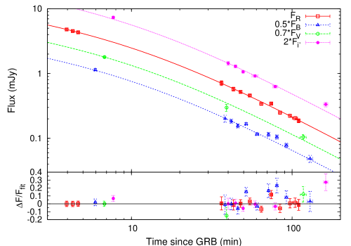
Figure 6: Top panel: $BVRi^{\prime}$ multi-colour light curve of GRB 051111 acquired by FTN (observer frame). Solid line shows the best smooth broken power-law fit of $R$ points (see text). Bottom panel: fractional residuals with respect to the fit.

$$F(t)=\frac{F_{0}}{(t/t_{\rm b})^{\alpha_{1}}+(t/t_{\rm b})^{\alpha_{2}}}$$ (1)

The best-fit parameters resulted: $\alpha_{1}=0.35\pm 0.08$, $\alpha_{2}=1.35\pm 0.04$, $t_{\rm b}=11.5\pm 0.5$ minutes ($\chi^{2}/{\rm dof}=10.0/9$; see solid line of Fig. 6). The value derived for the break time is consistent with that found for the $R$ band by Butler et al. (Butler06 (2006)). The light curves of the other filters are not sampled comparably well particularly at the beginning of observations. We then fitted the other filters light curves by leaving only the normalisation free to vary and fixing $\alpha_{1}$, $\alpha_{2}$, $t_{\rm b}$ to their correspondent values found for the $R$ filter. In all cases the $\chi^{2}$ turned out to be acceptable. Figure 6 shows all these best-fit broken power laws, therefore consistent with no colour evolution. The bottom panel of Fig. 6 shows the fractional residuals for each of the optical bands with respect to their best-fit function, respectively. The extrapolation of the $R$ light curve to $\sim 1000$ minutes after the burst is consistent within uncertainties with the observations reported by Nanni et al. (Nanni05 (2005)) in the $R_{c}$ filter, ruling out the possibility of other breaks before $10^{3}$ minutes. We note the possible presence of two humps in the $B$ and $R$ light curves: the first comprises a 10–20% excess above the expected flux from the power law fit between 70 and 90 minutes and the second occurs at 40–50 minutes with flux at 5–10% in excess of the fit. If we repeat the fit by ignoring these points, the best-fit normalisation decreases by $\sim$5%, so that the corresponding excesses increase by the same percentage. Around 170 minutes we have a single point in $B$ which is $(25\pm 10)$% in excess of the fit $B$ (2.5$\sigma$). Interestingly, also Butler et al. (Butler06 (2006)) found similar residual variability in the optical bands at $\geq 30$% around the best-fitting broken power-law model at $t>200$ minutes. Alternatively, if we fix $\alpha_{2}=\alpha_{\rm x,\gamma}$, the fit of the R light curve turns out to be equally good ($\chi^{2}/{\rm dof}=10.3/10$), with $\alpha_{1}=0.61\pm 0.10$ and $t_{\rm b}=36\pm 20$ minutes. However, if we fit the light curves of the other filters by allowing just the normalisation free to vary, we find acceptable fits, except for $i^{\prime}$, for which the fit is bad ($\chi^{2}/{\rm dof}=18.0/6$, chance probability of $6\times 10^{-3}$).

4 Spectral Energy Distribution

Given the lack of evidence for dramatic colour changes during observations, we found an epoch suitable to study the Spectral Energy Distribution (SED) of the GRB afterglow. To this aim, we made use of IR observations reported by Bloom et al. (Bloom05 (2005)) in the $J$, $H$ and $K_{s}$ filters, carried out between 83.9 and 88.7 minutes after the GRB. The optimum time at which to calculate the SED, when several measurements at different wavelengths were made suitably closely in time, was chosen to be t${}_{\rm SED}=80$ min. We back-extrapolated the values reported by Bloom et al. (Bloom05 (2005)) to $t_{\rm SED}$ assuming a power-law decay with $\alpha_{2}=1.35$ derived from fitting the $R$ band (Sec. 3.4). We corrected for a small Galactic extinction, following Cardelli et al. (Cardelli89 (1989)): $A_{J}=0.14$, $A_{H}=0.09$ and $A_{Ks}=0.06$. We finally converted magnitudes into fluxes following Campins et al. (Campins85 (1985)). Optical $BVRi^{\prime}$ magnitudes have been interpolated linearly to $t_{\rm SED}$ taking the measurements just before and after it. X-ray observations began 15 minutes after $t_{\rm SED}$: we back-extrapolated the X-ray flux assuming the simple best-fit power-law derived from X-ray data, with $\alpha_{\rm x}=1.56\pm 0.08$ (Sec. 3.2). The errors on $\alpha_{\rm x}$ and normalisation, which are correlated, have been propagated to estimate the uncertainty on the extrapolated X-ray flux. The X-ray spectral shape is that of the spectrum at $t=95$ min and rescaled according to the back-extrapolation factor. We ignored rest-frame X-ray frequencies below $4.6\times 10^{17}$ Hz (i.e., 1.9 keV) because these are partially affected by significant $N_{\rm H}$. The resulting SED is shown in Fig. 7.

Figure 7: Rest-frame Spectral Energy Distribution at 80 min after the burst from observed IR (Bloom et al. Bloom05 (2005)) to X-rays measured with Swift/XRT. A simple power law fits the spectrum with an index $\beta_{\rm o,x}=0.84\pm 0.02$ (thin solid line, $\chi^{2}/{\rm dof}=6.0/9$). Fluxes have been corrected for Galactic extinction. Alternatively, the broken power-law fit is shown when significant intrinsic extinction is modelled: dashed line corresponds to the SMC profile, both extinguished (thin line) and when the extinction is taken out (thick line). Dashed-dotted line shows the result with a Q2 profile: extinguished (thin line) and when the extinction is taken out (thick line). See Table 4.

We fitted the whole SED with a simple power law, $F(\nu)\sim\nu^{-\beta}$: $\beta_{\rm o,x}=0.84\pm 0.02$ ($\chi^{2}/{\rm dof}=6.0/9$). If we fit IR/optical and X-ray measurements with separate power laws, it results: $\beta_{\rm o}=0.76\pm 0.07$ and $\beta_{\rm x}=\Gamma_{\rm x}-1=1.15\pm 0.15$ ($\chi^{2}/{\rm dof}=4.3/7$).

We also fitted the SED with a broken power law with $\beta_{\rm o}-\beta_{\rm x}=0.5$, assuming a number of extinction profiles accounting for possible intrinsic extinction. The results are discussed in Sec. 4.2 and reported in Table 4.

4.1 Element abundances and column densities

From the Keck optical absorption spectrum Penprase et al. (Penprase06 (2006)) measure a Zn column density of $\log{(N_{\rm ZnII})}=13.58\pm 0.15$ cm^-2. Because of the redshift, the Lyman $\alpha$ feature does not fall within the Keck optical band, so that the $N_{\rm HI}$ cannot be measured directly, unlike other GRBs (see e.g. Vreeswijk et al. Vreeswijk04 (2004), Starling et al. Starling05 (2005), Chen et al. Chen05 (2005), Fynbo et al. Fynbo06 (2006)). They assume a $\approx$1/10 solar metallicity typical of QSO-DLA systems, i.e. [Zn/H]$\approx-1$ and find $N_{\rm H}\sim 7.9\times 10^{21}$ cm^-2. The soft X-ray photoelectric cutoff measured in terms of $N_{\rm H}$ actually is a measure of the metals column density $N_{\rm Z}$ under the assumption of solar metallicity (Morrison & McCammon Morrison83 (1983)). In particular, the soft X-ray absorption is mainly due to $\alpha$ metals and secondly to the Fe-peak metals, with no distinction between dust and gas. Oxygen K-shell absorption edges represent the main contribution in the XRT energy band in the assumption of relative solar abundances. The relative contributions to the total absorption also depend on redshift, given that the 0.2–10 keV energy band considered is fixed with respect to the observer frame. Hereafter we adopt the solar abundances as given by Asplund et al. (Asplund05 (2005)). If we fit the X-ray spectrum by fixing the metallicity to be 1/10 solar, the resulting $N_{\rm H}$ is significantly higher than that derived by Penprase et al. (Penprase06 (2006)) (see Table 3).

If, however, we adopt a solar metallicity, the $N_{\rm H}$ derived from X-rays, $8.0_{-2.6}^{+3.3}\times 10^{21}$ cm^-2, is consistent with the value derived by Penprase et al. (Penprase06 (2006)), although based on an incompatible metallicity assumption. Possibly, this could be explained by a significant fraction of molecular gas: in fact, Arabadjis & Bregman (Arabadjis99 (1999)) and Baumgartner & Mushotzky (Baumgartner06 (2006)) found that in the Milky Way for column densities higher than $10^{21}$ cm^-2 the X-ray column densities are 1.5–3 times as high as those derived from radio/optical. Alternatively, Zn depletion into dust could possibly explain this. However, apart from the cool dense ISM, in which the zinc fraction in dust grains can be as high as 20% ISM (Savage & Sembach Savage96 (1996)), Zn depletion is usually negligible and no evidence for it has been found in GRB-DLAs so far. The cool dense ISM is incompatible with the depletion pattern of the warm disk found by Penprase et al. (Penprase06 (2006); see below, this Section). Another possibility to reconcile the mismatch between metallicity and X-ray absorption is to allow X-ray absorbing elements to be overabundant with respect to the measured Zn: e.g, an overabundance of $\alpha$ metals with respect to zinc, as it appears to be the case for GRB 050401 (Watson et al. Watson06 (2006)). However, in the case of GRB 051111 it would be difficult to explain why silicon is not very abundant: from table 2 of Penprase et al. (Penprase06 (2006)) we take $\log{({\rm Si})}=16.18\pm 0.20$ and $\log{({\rm Zn})}=13.58\pm 0.15$. It follows that [Si/Zn]$=\log{({\rm Si}/{\rm Zn})}-\log{({\rm Si}/{\rm Zn})_{\odot}}=-0.30\pm 0.25$ and this could hardly be accounted for as due to dust depletion only. Another possibility is an overabundance of oxygen, as the $\alpha$ element mainly responsible for the X-ray absorption. We measure the O abundance directly and we compare it with that of Zn, which we know from the Keck optical spectrum because it is non-refractory to dust depletion. From the $N_{\rm H}=8.0_{-2.6}^{+3.3}\times 10^{21}$ cm^-2 measured assuming solar metallicity, we derive an O column density of $\log{({\rm O})}=18.56\pm 0.18$, i.e. [O/Zn]$=\log{({\rm O}/{\rm Zn})}-\log{({\rm O}/{\rm Zn})_{\odot}}=0.9\pm 0.2$. The O column density value estimated assuming $N_{\rm H}=7.1_{-2.4}^{+3.2}\times 10^{22}$ cm^-2 (from Table 3) and a metallicity of 1/10 solar is equivalent within the errors: the oxygen is 10 times less abundant and the $N_{\rm H}$ column density is $9\pm 5$ times higher. If we alternatively assume the lowest value we obtained, i.e. in the 0.3–10 keV ignoring the channel from 0.43 to 0.6 keV, $N_{\rm H}=5.1_{-2.1}^{+2.9}\times 10^{21}$ cm^-2, the relative oxygen abundance with respect to zinc turns out to be [O/Zn]=$0.7\pm 0.3$.

The value of [O/Zn] can be compared with [$\alpha$/Zn]$=0.5\pm 0.2$ found by Watson et al. (Watson06 (2006)) for GRB 050401. If this is also true for GRB 051111, we do not know a mechanism that can explain the observed overabundance of oxygen with respect to other $\alpha$ elements, e.g. either [O/Si]=$1.2\pm 0.3$ ([O/Si]=$1.0\pm 0.4$) assuming $N_{\rm H}=8.0_{-2.6}^{+3.3}\times 10^{21}$ cm^-2 ($N_{\rm H}=5.1_{-2.1}^{+2.9}\times 10^{21}$ cm^-2).

As we do not have a direct measure of either O or H, we have to assume both [O/H] and [Zn/H], provided that eq. 2 is satisfied:

$$[{\rm O}/{\rm H}]-[{\rm Zn}/{\rm H}]=[{\rm O}/{\rm Zn}]$$ (2)

From the low column densities of Fe, Cr, Si and Mn compared with Zn, Penprase et al. (Penprase06 (2006)) infer a strong dust depletion, in agreement with what found for other GRBs (Savaglio & Fall Savaglio04 (2004)). The depletion pattern matches that of a warm disk (WD) and marginally that of a warm disk plus halo (WDH) observed in the Milky Way (see e.g. Savaglio et al Savaglio03 (2003) and references therein). From the 1/10 solar metallicity assumption, Penprase et al. (Penprase06 (2006)) estimate a dust-to-gas ratio of about 1/12 that of the Milky Way and from their value of the $N_{\rm H}$ they derived an extinction of $A_{V}\approx 0.55$.

It must be pointed out that the measure of the ZnII column density by Penprase et al. (Penprase06 (2006)) has not universally been accepted (Prochaska Prochaska05 (2005, 2006), Prochaska et al. Prochaska06b (2006)); in particular, according to Prochaska et al. (Prochaska06b (2006)) both ZnII and SiII are saturated and they derive a lower limit on the amount of zinc: $\log{(N_{\rm ZnII})}>13.71$ cm^-2, i.e. about 1$\sigma$ above what obtained by Penprase et al. (Penprase06 (2006)). Here, we do not discuss the reasons for these different conclusions; rather, we note that in this case it would be [O/Zn]$<0.8$ and the evidence for overabundant oxygen would be much less compelling. Also the optical extinction mentioned above would become merely a lower limit: $A_{V}>0.55$.

4.2 Host extinction

According to the afterglow broad band spectrum expected in the fireball model (Sari et al. Sari98 (1998)), we assume a straight power law, $F_{\nu}\sim\nu^{-\beta}$, or a broken power law with $\Delta\beta=0.5$ in the typical scenario of slow cooling with the cooling frequency $\nu_{\rm c}$ lying between optical and X-rays (see Sec. 5). However, the possible dust extinction due either to the circumburst environment and/or the host galaxy not only suppresses the optical flux but also reddens it in a way which reflects the properties of dust. As a result, $\beta_{\rm o}$ measured in the optical domain may be significantly steeper than the intrinsic one, $\beta_{\rm o,i}$, we would have measured in the absence of extinction ($A_{V}=0$). The values for $A_{V}$ and $\beta_{\rm o,i}$ as estimated from fitting the SEDs of GRBs are to some degree correlated, as proved by previous studies: e.g., see Panaitescu (Panaitescu05 (2005)), Stratta et al. (Stratta04 (2004)) and Kann et al. (Kann06 (2006)). In order to account for possible intrinsic extinction, we fitted the SED with the following general law (eq. 3):

$$F_{\nu}=F_{0}(\nu)\ 10^{-0.4A(\nu)}$$ (3)

where $F_{0}(\nu)$ is the afterglow spectrum in the absence of extinction: $F_{0}(\nu)\propto\nu^{-\beta_{\rm o,i}}$ ($\beta_{\rm x}=\beta_{\rm o,i}$) in the power-law case, $F_{0}(\nu)\propto\nu^{-\beta_{\rm o,i}}$ (for $\nu<\nu_{0}$) and $F_{0}(\nu)\propto\nu^{-\beta_{\rm x}}$ ($\beta_{\rm x}=\beta_{\rm o,i}+0.5$, for $\nu>\nu_{0}$) in the broken power-law case ($\nu_{0}$ is the break frequency). $A(\nu)$ is the extinction profile as a function of $\nu$ and depends on the dust model assumed.

We tried to account for intrinsic extinction assuming nine different extinction profiles:

1. Milky Way (MW) using the parameterisation by Pei (Pei92 (1992)), yielding $N_{\rm H}/A_{V}=1.6\times 10^{21}$ cm^-2.

2. Large Magellanic Cloud (LMC) using the parameterisation by Pei (Pei92 (1992)), yielding $N_{\rm H}/A_{V}=7.6\times 10^{21}$ cm^-2.

3. Small Magellanic Cloud (SMC) using the parameterisation by Pei (Pei92 (1992)), yielding $N_{\rm H}/A_{V}=1.5\times 10^{22}$ cm^-2.

4. The “Q1” curve by Maiolino et al. (Maiolino01 (2001)) derived for population of dust grains whose size distribution is given by a power law, $dn/da\propto a^{-q},(a_{\rm min}\leq a\leq a_{\rm max})$, where $q=3.5$, $a_{\rm min}=0.005$ $\mu$m, $a_{\rm max}=10$ $\mu$m. It is $N_{\rm H}/A_{V}=6.7\times 10^{21}$ cm^-2 assuming a standard gas-to-dust ratio in the ISM.

5. The “Q2” curve by Maiolino et al. (Maiolino01 (2001)) derived under the same assumptions as for the Q1 profile, but the following parameters: $q=2.5$ $a_{\rm max}=1$ $\mu$m. It is $N_{\rm H}/A_{V}=3.3\times 10^{21}$ cm^-2 assuming a standard gas-to-dust ratio in the ISM.

6. SN extinction profile taken from Maiolino et al. (Maiolino04 (2004)) for the case of a $10M_{\odot}$ SN with solar metallicity (for our purposes this case is similar to the other SN profiles discussed by those authors).

7. The type I extinction law (hereafter CLW1) provided by Chen et al. (Chen06 (2006)), derived assuming a dust mainly composed by graphite and silicate grains following a power law multiplied by an exponential, $dn/da\propto a^{-q}e^{a/a_{c}},(a_{\rm min}\leq a\leq a_{\rm max})$, where $a_{\rm min}=0.05$ $\mu$m, $a_{\rm max}=2.5$ $\mu$m, $q=2.61$ and $a_{c}=0.21$ $\mu$m.

8. The type II extinction law (hereafter CLW2) provided by Chen et al. (Chen06 (2006)), under the same assumptions as for CLW1, but the following parameters: $q=3.09$ and $a_{c}=0.29$ $\mu$m.

9. This extinction law corresponds to a power law, $A(\nu)=A_{V}(\nu/\nu_{V})^{\gamma}$, as proposed by Savaglio & Fall (Savaglio04 (2004)) for GRB 020813. Since the fitting procedure in the case of our data does not constrain very well the two parameters $A_{V}$ and $\gamma$, we fixed $\gamma$ in two boundary cases found by Savaglio & Fall (Savaglio04 (2004)), i.e. $\gamma=0$ and $\gamma=0.85$. Hereafter the two cases are referred to as SF($\gamma=0$) and SF($\gamma=0.85$).

Figure 8: Extinction profiles of eight different laws: SMC (thin solid line), LMC (thin dashed line), MW (thin dotted line), Q1 (thick solid line), the absolute extinction expected for a $10M_{\odot}$ solar metallicity SN profile from Maiolino et al. (Maiolino04 (2004)) (thick dashed-dotted line), CLW1 (thin dashed-dotted line), CLW2 (thick dashed line), Q2 (thick dotted line).

The first eight extinction curves listed above considered are shown in Fig. 8. The results are reported in Table 4.

Table 4: Best-fit results of the IR-optical-X SED at $t=80$ minutes. Uncertainties are at 90% CL.

Model(a)	Extinction	$A_{V}^{(b)}$	$\beta_{\rm o,i}$	$\nu_{0}^{(c)}$	$\chi^{2}/{\rm dof}$
	Law			($10^{15}$ Hz)
PL	Unextinguished	0	$0.84\pm 0.02$	–	6.0/9
PL	SMC	$<0.02$	$0.84\pm 0.02$	–	13.6/8
PL	LMC	$<0.02$	$0.84\pm 0.02$	–	13.6/8
PL	MW	$<0.03$	$0.84\pm 0.02$	–	13.6/8
PL	Q1	$<0.05$	$0.84\pm 0.02$	–	13.6/8
PL	Q2	$<0.19$	$0.84\pm 0.03$	–	13.6/8
PL	CLW I	$<0.03$	$0.84\pm 0.02$	–	13.6/8
PL	CLW II	$<0.03$	$0.84\pm 0.02$	–	13.6/8
PL	SN 10 $M_{\odot}$	–	$0.88\pm 0.02$	–	225/9
PL	SF($\gamma=0.0$)	$<0.34$	$0.84\pm 0.04$	–	13.6/8
PL	SF($\gamma=0.85$)	$<0.03$	$0.84\pm 0.02$	–	13.6/8
BKN PL	Unextinguished	0	$0.70_{-0.01}^{+0.09}$	$134_{-94}^{+312}$	12.95/8
BKN PL	SMC	$0.16_{-0.11}^{+0.06}$	$0.47_{-0.05}^{+0.18}$	$3.0_{-1.6}^{+52}$	7.7/7
BKN PL	LMC	$0.21_{-0.13}^{+0.05}$	$0.44_{-0.03}^{+0.18}$	$1.8_{-0.6}^{+30}$	6.4/7
BKN PL	MW	$0.20_{-0.05}^{+0.06}$	$0.43_{-0.03}^{+0.20}$	$1.5_{-0.5}^{+30}$	6.4/7
BKN PL	Q1	$0.39_{-0.10}^{+0.11}$	$0.46_{-0.05}^{+0.18}$	$1.5_{-0.5}^{+34}$	6.7/7
BKN PL	Q2	$1.29_{-0.45}^{+0.53}$	$0.54_{-0.06}^{+0.07}$	$1.1_{-0.1}^{+1000}$	8.8/7
BKN PL	CLW I	$0.30_{-0.28}^{+0.09}$	$0.48_{-0.09}^{+0.22}$	$2.9_{-1.9}^{+1000}$	9.8/7
BKN PL	CLW II	$0.25_{-0.20}^{+0.08}$	$0.47_{-0.08}^{+0.20}$	$2.4_{-1.4}^{+1000}$	8.8/7
BKN PL	SN 10 $M_{\odot}$	–	$0.46\pm 0.02$	$1.7_{-0.4}^{+0.3}$	78/8
BKN PL	SF($\gamma=0.0$)	$1.8_{-0.6}^{+0.9}$	$0.60_{-0.08}^{+0.12}$	$1.0_{-0.0}^{+1000}$	11.4/7
BKN PL	SF($\gamma=0.85$)	$0.26_{-0.18}^{+0.08}$	$0.46_{-0.03}^{+0.18}$	$2.0_{-0.7}^{+42}$	7.5/7

5 Discussion

In order to interpret the light curves and spectra at different epochs for different energy bands according to the standard fireball model, we consider the two usual cases of different medium density profile, $\rho\propto r^{-k}$: ISM (Sari et al. Sari98 (1998)) ($k=0$) vs. Wind (Chevalier & Li Chevalier99 (1999)) ($k=2$). Hereafter, $\nu_{m}$ and $\nu_{c}$ are the peak synchrotron energy corresponding to the minimum energy of the electron energy distribution ($dN/d\gamma\propto\gamma^{-p}$, for $\gamma>\gamma_{m}$, where $p$ is the electron energy distribution index) and the cooling frequency, where the electrons lose their energy within the dynamical timescale, respectively. Likewise, $\nu_{\rm o}$ and $\nu_{\rm x}$ are the optical and X-ray frequencies, respectively.

First of all, we briefly discuss whether a break frequency lies between optical and X-rays at 80 minutes. As reported in Sec. 4, a single power-law fit from optical to X-rays is acceptable with $\beta_{\rm o,x}=0.84\pm 0.02$. However, despite the goodness of the fit, the optical and X-ray indices alone, $\beta_{\rm o}=0.76\pm 0.07$ and $\beta_{\rm x}=1.15\pm 0.15$, seem to support a break consistent with $\beta_{\rm x}-\beta_{\rm o}=0.5$, often expected in the fireball model. Hence, although the single power law cannot be ruled out at all, it seems disfavoured. Notably, in the case of a single power law, an important consequence would be the negligible optical extinction: $A_{V}<0.05$ (90% CL) for almost all of the extinction profiles considered (see Table 4), unless one assumes very flat profiles around $1\times 10^{15}$ Hz, such as the Q2 and SF($\gamma=0$) (see Fig. 8) for which it is $A_{V}<0.19$ and $A_{V}<0.34$, respectively. Given the high column densities of metals and the significant X-ray absorption measured, this appears to be hardly the case. In contrast, a broken power law seems to better allow for a higher extinction: the models based on big dust grains give values of $A_{V}$ between 0.25 and 1.29 and, in particular, the grey extinction (Stratta et al. Stratta04 (2004)) power-law profiles considered by Savaglio & Fall (Savaglio04 (2004)) can account for even higher values, ranging from 0.26 to 1.8.

Hence the broken power-law case seems to be more consistent with the amount of extinction expected from the significant dust depletion measured in the optical spectrum: $A_{V}\sim 0.55$ or even much higher, as discussed in Sec 4.1.

From these considerations, in the following we consider the alternative of a break frequency between optical and X-rays, which appears to be more likely for the SED at 80 minutes.

• $\nu_{\rm x}<\nu_{c}$

  At $t_{\rm SED}$, i.e. after the break in the optical light curve, the case $\nu_{m}<\nu_{\rm x}<\nu_{c}$ is unlikely to describe the data. If $\nu_{\rm o}<\nu_{m}<\nu_{\rm x}<\nu_{c}$, we should expect $\beta_{\rm o,i}=-1/3$ (all cases), which is inconsistent with our results (Table 4). Alternatively, if $\nu_{m}<\nu_{\rm o}<\nu_{\rm x}<\nu_{c}$, then it must be $\beta_{\rm o,i}=\beta_{\rm x}$. From Table 4 the only solution is the case of a single power law from optical to X-ray and it is $\beta_{\rm o,i}=\beta_{\rm x}=0.84\pm 0.02$. For both $k=0,2$ cases, it should be $\beta_{\rm x}=(p-1)/2$, implying $p=2.68\pm 0.04$. The measured value for $\alpha_{\rm x}$ of $1.56\pm 0.08$ is inconsistent with that expected for the ISM case, namely $3(p-1)/4=1.26\pm 0.03$, but is very marginally consistent (2% significance) with the Wind case: $(3p-1)/4=1.76\pm 0.03$. This, combined with the negligible extinction implied by the single power law case (Table 4), makes this scenario unlikely.

• $\nu_{c}<\nu_{\rm x}<\nu_{m}$ (fast cooling)

  In all cases, it should be $\beta_{\rm x}=1/2$, clearly incompatible with data.

• $\nu_{c}<\nu_{m}<\nu_{\rm x}$ (fast cooling)

  In this case, following Sari et al. (Sari98 (1998)) we should expect a previous break in the X-ray light curve from $\alpha_{\rm x}=1/4$ to $\alpha_{\rm x}=(3p-2)/4$ when $\nu_{m}$ crossed the X-ray band. Furthermore, when at earlier epoch $\nu_{c}$ crossed the X-ray band, the X-ray light curve should have been even shallower, with $\alpha=-1/6$. All this is at odds with the X-ray light curve inferred from Fig. 4.

• $\nu_{m}<\nu_{c}<\nu_{\rm x}$ (slow cooling)

  In both cases, it is $\beta_{\rm x}=p/2$, yielding $p=2.3\pm 0.3$. This implies $\alpha_{\rm x}=(3p-2)/4=1.22\pm 0.22$. This is compatible with the measured $1.56\pm 0.08$ within 1.5 $\sigma$, although somewhat shallower. The case of $\nu_{\rm o}<\nu_{m}$ has already been ruled out because the expected optical decay ($\alpha=-1/2$ or $0$ for $k=0,2$, respectively) is too shallow compared with the measured decay ($\alpha_{2}$). Hence, hereafter we consider the case $\nu_{m}<\nu_{\rm o}<\nu_{c}<\nu_{\rm x}$. For both cases, it is $\beta_{\rm o,i}=(p-1)/2=0.65\pm 0.15$. This value is in agreement with most of those obtained by fitting the SED (see Table 4). The expected optical decay power-law index is $\alpha_{\rm o}=3(p-1)/4=1.0\pm 0.2$ (ISM) and $\alpha_{\rm o}=(3p-1)/4=1.5\pm 0.2$ (Wind), which favours the Wind profile, given that $\alpha_{2}=1.35\pm 0.04$. In the Wind case, the optical decay should be steeper than the X-ray decay by 0.25; the observed difference, $\alpha_{2}-\alpha_{\rm x}=-0.2\pm 0.1$, could be indicative of a stratified wind, but the observed pre-break optical decay would be difficult to explain in this scenario. See Sec. 5.1.2.

5.1 Break in the optical light curve

The interpretation of the optical break as the result of the passage of the cooling frequency across the optical bands appears to be unlikely, because we observe $\Delta\alpha\sim 1$ to be compared with 0.25 expected in that case. The passage of $\nu_{m}$ cannot explain it either, as the expected pre-break slope should be positive (specifically, $\alpha_{1}=-0.5$), which is definitely not the case. The break is unlikely due to a jet, given the different behaviour exhibited by the X-ray afterglow decay, which seems to rule out the achromatic nature, required by the jet scenario, not to mention that a break time of $\sim 12$ minutes would be unusually early. In the following we discuss the optical break in comparison with the X-ray behaviour in an attempt to explain it in a single framework.

5.1.1 Breaks in the X-ray power-law decay

If we consider the connection between the $\gamma$-ray tail of the prompt emission and the late X-ray afterglow as due to chance, it is natural to assume that X-rays mimic the optical decay: in this case, after the prompt emission the X-ray decay would be steeper than $\alpha_{{\rm x},\gamma}=1.54$, followed by a shallow decay phase and finally reconnecting to the normal decay measured $\alpha_{\rm x}=1.56$. This seems consistent with the slope observed during the tail of the prompt emission, $\alpha_{\gamma}=1.8\pm 0.2$, which is marginally steeper than $\alpha_{{\rm x},\gamma}$. The steep-shallow-normal behaviour has been observed with Swift for many early X-ray afterglows. The steep decay in the early phase is interpreted as tail of the prompt emission and not produced by the interaction of the fireball with the surrounding medium, as for the afterglow (Kumar & Panaitescu Kumar00 (2000); Tagliaferri et al. Tagliaferri05 (2005); Lazzati & Begelman Lazzati06 (2006)). The following shallow X-ray decay would be the result of a continuous energy injection at the end of which there is a steepening in the light curve (Nousek et al. Nousek06 (2006); Zhang et al. Zhang06 (2006)). In this case, GRB 051111 would represent one of the few cases in which this behaviour, typical of early X-ray afterglows, is seen in the early optical afterglow. This scenario for GRB 051111 seems to be supported also by the ROTSE observations (Yost et al. Yost06 (2006)) as well as by the data taken with the Katz Automatic Imaging Telescope (KAIT) reported by Butler et al. (Butler06 (2006)).

The alternative description of the X-ray light curve in terms of a double broken power model reported in Sec. 3.2 fits the possible X-ray bump visible around 600 minutes, followed by a possible steepening. In principle, these variations with respect to the simple power-law fit may be explained in terms of a minor late energy injection process, responsible for a short-lived shallow decay, or alternatively, as due to the narrow component of a two-component jet (e.g. Huang et al. Huang04 (2004), Granot Granot05 (2005)). However in the latter case from simultaneous and late optical observations (Butler et al. Butler06 (2006), Nanni et al. Nanni05 (2005)) the expected steepening after the putative second break at $\sim 600$ minutes is not evident. Unfortunately, the late X-ray upper limit shown in Fig. 4 is not conclusive.

5.1.2 Single X-ray power-law decay

Alternatively, as shown in Sec. 3.3, one may consider that the tail of the prompt event connects with the late X-ray afterglow light curve with a single power-law slope of $\alpha_{{\rm x},\gamma}=1.54\pm 0.10$. Although the X-ray data gap until XRT observations do not exclude breaks in the power law as found for many Swift early X-ray afterglows (O’Brien et al. OBrien06 (2006)), it seems unlikely that in case of variations the two data sets would connect so well despite 2–3 orders of magnitude difference in fluxes. A single power law connecting the BAT $\gamma$-ray tail with the XRT afterglow has already been observed for some GRBs: e.g. GRB 050721, GRB 050726, GRB 050801 and GRB 050802, see fig. 3 of O’Brien et al. (OBrien06 (2006)). Also for the very first GRB for which an afterglow was found, GRB 970228, the X-ray power-law back-extrapolation to the time of the burst nicely connects with the X-ray prompt emission (Costa et al. Costa97 (1997)). Therefore, in this section we discuss the case in which there is no break in the X-ray light curve simultaneous to that in the optical band. The different decay rates of optical and X-rays require the presence of a break frequency in between, as already argued above. Here we also assume that there is no significant spectral X-ray evolution from the prompt emission tail to the XRT, i.e. $\beta_{\rm x}$ being constant. This is not at odds with $\beta_{\gamma}=0.44$ measured during the $\gamma$-ray tail: e.g., in the case of GRB 050726 we have $\beta_{\gamma}=0.01\pm 0.17$ and $\beta_{\rm x}=0.94\pm 0.07$ (O’Brien et al. OBrien06 (2006)).

A possible explanation of the optical break with no corresponding break in the X-ray light curve is when the afterglow front shock passes from ISM to a Wind environment. In this case we would expect a steepening of 0.5 in the optical bands only (because $\nu_{c}<\nu_{\rm x}$). However the measured $\Delta\alpha$ is about 1. If we consider the more general case of density scaling as $r^{-k}$, the expected steepening due to passage from ISM to Wind is $\Delta\alpha=k/(8-2k)$, i.e. $k\approx 2.7$. This solution has been suggested to explain the similar case of GRB 060206 in which an optical break with no corresponding X-ray break was observed (Monfardini et al. Monfardini06 (2006)). However, in this case ($k>2$) the X-ray decay $\alpha_{{\rm x},\gamma}$ should be smaller by at least $0.25$ than the optical $\alpha_{2}$, while we find $\alpha_{{\rm x},\gamma}-\alpha_{2}=0.19\pm 0.11$.

Alternatively, the post-break decay index (optical and X-ray) themselves can be explained if we assume $p=2.75$ and $k=1/2$. The essential problem for the ISM-wind transition (stratified wind) model is that the pre-break optical decay index $\alpha_{1}=0.35$ is too shallow. In a more generalised model, a stratified wind model might include a transition from $k<0$ (increasing density with radius) to $k>0$. Compared with the ISM ($k=0$), this should give a shallower pre-break optical decay. From table 5 in Yost et al. (Yost03 (2003)), in the case $\nu_{m}<\nu_{\rm o}<\nu_{\rm c}$, the decay index $\alpha_{\rm o}$ for the Wind model is given by $\alpha_{\rm o}=3p/4-[(12-5k)/(16-4k)]>3p/4-5/4=0.81$ ($p=2.75$) or $0.48$ ($p=2.3$). Therefore the observed pre-break optical decay is too shallow to satisfy this scenario.

A transition from ISM to a wind environment in principle may occur when, for instance, a He merger progenitor, beginning with a massive star with strong winds, travels up to 10 pc from the wind environment before the GRB explosion (Fryer et al. Fryer06 (2006)). In this scenario, the progenitor should have run away from the line of sight to the observer. Alternatively, the possibility of a binary system with a Wolf-Rayet star seems more unlikely to produce such an environment, because of the strong wind dominating that of the companion (van Marle et al. vanMarle06 (2006)), unless one considers a double Wolf-Rayet system, which would be very rare.

Finally, in this scenario, there is another aspect hard to reconcile with the overall picture: if the tail of the prompt emission is the beginning of the afterglow, then the $\gamma$-ray spectral index, $\beta_{\gamma}=0.44$, and the power-law decay index, $\alpha_{{\rm x},\gamma}=1.54$, appear to be incompatible with the synchrotron shock model interpreted as produced by external shocks.

5.2 The $\gamma$-ray tail

Interestingly, Giblin et al. (Giblin02 (2002)) studied the $\gamma$-ray tail of a number of FRED-like GRBs detected with BATSE (Paciesas et al. Paciesas99 (1999)). They tested whether the decay rate and the spectrum are consistent with the expectations of an early high-energy afterglow synchrotron emission due to external shocks. Their results show that about 20% of the GRBs considered are consistent with it, in particular with the evolution expected for a jet.

In the jet case, the power-law decay index, $\alpha_{\gamma}=1.8$, should correspond to $p$, provided that $p>2$. As it is not the case, we have to apply the formalism by Dai & Cheng (Dai01 (2001)) for $p<2$, according to which we have two possible closure relations: $4\alpha_{\gamma}-2\beta_{\gamma}-7=0$ ($\nu_{\gamma}<\nu_{c}$), or $4\alpha_{\gamma}-2\beta_{\gamma}-6=0$ ($\nu_{\gamma}>\nu_{c}$). In either case, they turn out to be acceptable within uncertainties: $-0.7\pm 0.8$ yielding $p=1.9\pm 0.1$ and $0.3\pm 0.8$ yielding $p=0.9\pm 0.1$, for the $\nu_{\gamma}<\nu_{c}$ and $\nu_{\gamma}>\nu_{c}$ cases, respectively. This result shows that the tail of the prompt emission is consistent with the jet case, as found by Giblin et al. (Giblin02 (2002)) for some FREDs by BATSE. It must be pointed out, however, that the values for $p$ in this case seem incompatible with $2.3\pm 0.3$ derived from the optical/X-ray afterglow.

Curvature effects alone cannot account for the $\alpha_{\gamma}$ and $\beta_{\gamma}$ measured: in this case the expected closure relation $\alpha_{\gamma}-\beta_{\gamma}-2=0$ (e.g., Dermer Dermer04 (2004)) turns out to be $-0.6\pm 0.2$, incompatible with zero.

Notably, one of the GRBs studied by Giblin et al. (Giblin02 (2002)), GRB 910602, is strikingly similar to GRB 051111 in both temporal decay and spectrum: $\alpha_{\gamma}=1.74$ and $\beta_{\gamma}=0.52$. According to the classification of Giblin et al. (Giblin02 (2002)), this is a FRED with multi pulses near the peak. Also for this GRB, there is no softening along the tail and it appears to be inconsistent with the evolution of a spherical blast wave.

6 Conclusions

We provided a detailed study of the properties of both prompt emission and multi-wavelength early afterglow of a typical FRED burst detected by Swift. The optical afterglow light curve is fitted by a smooth broken power law, while little can be conclusively said about the simultaneous X-ray light curve. Interestingly, the flux of the $\gamma$-ray tail of the prompt emission, extrapolated in the 0.2–10 keV energy band, matches the back-extrapolation of the late X-ray afterglow with $\alpha_{{\rm x},\gamma}=1.54\pm 0.10$. We discussed two alternative cases, based on the behaviour of the X-ray afterglow light curve soon after the prompt event until $\sim$100 minutes, when XRT began observing.

If the connection between the tail of the prompt event and the late X-ray afterglow is pure chance, the $\gamma$-ray tail is the result of internal shocks and has no connection with the late X-ray afterglow. The X-ray afterglow light curve could mimic that measured in the optical, which monitors the shallow-to-normal decay phase observed in several early X-ray afterglows with Swift and interpreted as the gradual end of a continuous energy injection process into the front shock of the afterglow. In this case, this would be one of the first bursts, whose early optical afterglow shows the typical behaviour seen in X-rays. This interpretation seems to be consistent with other data sets (Butler et al. Butler06 (2006); Yost et al. Yost06 (2006)).

Alternatively, if the matching between $\gamma$-ray tail and the late X-ray afterglow is evidence for an early beginning of the X-ray afterglow during the tail of the prompt event, it is therefore sensible to assume no breaks in the X-ray light curve, while in contrast, the optical exhibits a break around 12 minutes after the burst. The break in the light curve observed only in the optical with $\Delta\alpha\sim 1$ could be the result of a passage from ISM to a Wind environment, $\rho\propto r^{-k}$, with $k\approx 2.7$. A weak point of this scenario is the fact that after the break the X-ray decay should be shallower than that of the optical by $0.25$ whereas we observe the optical decay index to be marginally steeper by $0.19\pm 0.11$. Alternatively, a stratified wind with $p=2.75$ and passing from a region of $k<0$ to $k>0$ could account for this, but the observed pre-break optical decay appears unaccountably shallow.

From the SED at 80 minutes, we find that the presence of the cooling frequency between optical and X-ray is consistent with significant intrinsic dust extinction inferred from the optical spectrum (Prochaska Prochaska05 (2005); Penprase et al. Penprase06 (2006)): $0.16\lesssim A_{V}\lesssim 0.21$ for standard extinction profiles (MW, SMC, LMC), or more probably $0.25\lesssim A_{V}\lesssim 1.8$ for dust dominated by big grains (Maiolino et al. Maiolino01 (2001); Chen et al. Chen06 (2006)) or grey extinction laws, as found for other GRBs (Stratta et al. Stratta04 (2004); Savaglio & Fall Savaglio04 (2004)). These kinds of extinction profiles might also be connected with dust destruction within a few tens of parsec of the GRB progenitor due to the intense UV and X-rays of the prompt emission, as suggested by several authors (Waxman & Draine Waxman00 (2000); Fruchter et al. Fruchter01 (2001); Perna et al. Perna03 (2003)).

In contrast, the absence of a spectral break between optical and X-ray would constrain the dust content ($A_{V}<0.19$), thus making it hard to reconcile with the column densities measured in the optical spectrum. Furthermore, it would also be hard to explain the different decay in X-rays ($\alpha_{\rm x}=1.54$) than in the optical after the break ($\alpha_{2}=1.35$). Thus, we conclude that the presence of the cooling break between optical and X-ray at 80 minutes after the burst is more likely than no break.

Although the content of some elements, as measured by optical spectroscopy, is a matter of ongoing debate (Penprase et al. Penprase06 (2006); Prochaska Prochaska05 (2005, 2006)), we use the X-ray absorption to infer either the overabundance of at least some of the $\alpha$ elements, like oxygen, or the presence of a significant amount of molecular gas along the line of sight through the host galaxy. This accounts for the high X-ray absorption and the amount of Zn measured in the optical as well as the measured dust depletion pattern.

We provided marginal evidence for the peculiarity of the circumburst environment of GRB 051111. The possible existence of a link between the class of the so-called FRED GRBs and the properties of the afterglow is supported by recent studies (Hakkila & Giblin Hakkila06 (2006); Bosnjak et al. Bosnjak06 (2006)), according to which these bursts are more likely to be associated with SNe. In light of this possibility, a thorough study of the properties of this class of GRBs could help shed light on this possible association.

- (1) Arabadjis, J.S., & Bregman, J.N. 1999, ApJ, 510, 806
- (2) Asplund, M., Gravesse, N., & Sauval, A.J., 2005, ASP Conf. Series, Vol. 336, 25
- (3) Baumgartner, W.H., & Mushotzky, R.F. 2006, ApJ, 639, 929
- (4) Berger, E., Penprase, B.E., Fox, D.B., Kulkarni, S.R., Hill, G., Schaefer, B., & Reed, M. 2005, ApJ, submitted (astro-ph/0512280)
- (5) Berger, E., Penprase, B.E., Cenko, S.B., et al. 2006, ApJ, 642, 979
- (6) Bessell, M.S. 1979, PASP, 91, 589
- (7) Beuermann, K., Hessman, F.V., Reinsch, K., et al. 1999, A&A, 352, L26
- (8) Bloom, J.S. 2005, GCN Circ. 4256
- (9) Bosnjak, Z., Celotti, A., Ghirlanda, G., Della Valle, M., & Pian, E. 2006, A&A, 447, 121
- (10) Butler, N.R., Li, W., Perley, D., et al. 2006, ApJ, accepted (astro-ph/0606763)
- (11) Campins, H., Rieke, G.H., & Lebovsky, M.J. 1985, AJ, 90, 896
- (12) Capalbi, M., Perri, M., Saija, B., & Tamburelli, F. 2005, “The Swift XRT Data Reduction User Guide”, http://swift.gsfc.nasa.gov/docs/swift/analysis
- (13) Cardelli, J. A., Clayton, G. C., & Mathis, J. S. 1989, ApJ, 345, 245
- (14) Chen, H.-W., Prochaska, J.X., Bloom, J.S., & Thompson, I.B. 2005, ApJ, 634, L25
- (15) Chen, S.L., Li, A.G., & Wei, D.M. 2006, ApJ, submitted (astro-ph/0603222)
- (16) Chevalier, R. A., & Li, Z.-Y. 1999, ApJ, 520, L29
- (17) Chincarini, G., Moretti, A., Romano, P., et al. 2005, ApJ, submitted (astro-ph/0506453)
- (18) Costa, E., Frontera, F., Heise, J., et al. 1997, Nature, 387, 783
- (19) Dai, Z. G., & Cheng, K. S. 2001, ApJ, 558, L109
- (20) Dermer, C.D. 2004, ApJ, 614, 284
- (21) Fishman, G.J., & Meegan, C.A. 1995, ARA&A, 33, 415
- (22) Fruchter, A., Krolik, J.H., & Rhoads, J.E. 2001, ApJ, 563, 597
- (23) Fryer, C.L., Rockefeller, G., & Young, P.A. 2006, ApJ, 647, 1269
- (24) Fukugita, M., Ichikawa, T., Gunn, J.E., et al. 1996, AJ, 111, 1748
- (25) Fynbo, J.P.U., Starling, R.L.C., Ledoux, C., et al. 2006, A&A, 451, L47
- (26) Galama, T.J., & Wijers, R.A.M.J. 2001, ApJ, 549, L209
- (27) Gehrels, N., Chincarini, G., Giommi, P., et al. 2004, ApJ, 611, 1005
- (28) Giblin, T.W., Connaughton, V., van Paradijs, J., et al. 2002, ApJ, 570, 573
- (29) Granot, J., 2005, ApJ, 631, 1022
- (30) Guidorzi, C., Monfardini, A., Gomboc, A., et al., 2006, PASP, 118, 288
- (31) Hakkila, J., & Giblin, T.W. 2006, ApJ, accepted (astro-ph/0604151)
- (32) Hill, G., Prochaska, J.X., Fox, D., Schaefer, B., Reed, M. 2005, GCN Circ. 4255
- (33) Huang, Y.F., Wu, X.F., Dai, Z.G., Ma, H.T., & Lu, T., 2004, ApJ, 605, 300
- (34) Kalberla, P.M.W., Burton, W.B., Hartmann, D., Amal, E.M., Bajaja, E., Morras, R., & Pöppel, W.G.L., 2005, A&A, 440, 775
- (35) Kann, D.A., Klose, S., & Zeh, A. 2006, ApJ, 641, 993
- (36) Krimm, A., Parsons, A.M., & Markwardt, C.B., 2004, “Swift BAT Ground Analysis Software Manual”, http://swift.gsfc.nasa.gov/docs/swift/analysis
- Krimm et al. (2005) Krimm, H., Ajello, M., Barbier, L., et al. 2005, GCN Circ. 4260
- (38) Kumar, P., & Panaitescu, A. 2000, ApJ, 541, L51
- (39) Landolt, A. U. 1992, AJ, 104, 340
- (40) La Parola, V., Mangano, V., Mineo, T., et al. 2005, GCN Circ. 4261
- (41) Lazzati, D., & Begelman, M.C. 2006, ApJ, 641, 972
- (42) Maiolino, R., Marconi, A., & Oliva, E. 2001, A&A, 365, 37
- (43) Maiolino, R., Schneider, R., Oliva, E., et al. 2004, Nature, 431, 533
- (44) Monfardini, A., Kobayashi, S., Guidorzi, C., et al. 2006, ApJ, 648, 1125
- (45) Morrison, R., & McCammon, D. 1983, ApJ, 270, 119
- (46) Mundell, C.G, Rol, E., Guidorzi, C., et al., 2005, GCN Circ. 4250
- (47) Nanni, D., Terra F., Bartolini, C., et al., 2005, GCN Circ. 4298
- (48) Nousek, J.A., Kouveliotou, C., Grupe, D., et al. 2006, ApJ, 642, 389
- (49) O’Brien, P.T., Willingale, R., Osborne, J., et al. 2006, ApJ, 647, 1213
- (50) Paciesas, W.S., Meegan, C.A., Pendleton, G.N., et al., 1999, ApJS, 122(2), 465
- (51) Panaitescu, A. 2005, MNRAS, 362, 921
- (52) Pei, Y.C. 1992, ApJ, 395, 130
- (53) Penprase, B.E., Berger, E., Fox, D.B., et al. 2006, ApJ, 646, 358
- (54) Perna, R., Lazzati, D., & Fiore, F. 2003, ApJ, 585, 775
- (55) Poole, T.S., Sakamoto, T., Blustin, A.J., Hancock, B., & Kennedy, T. 2005, GCN Circ. 4263
- (56) Prochaska, J.X. 2005, GCN Circ. 4271
- (57) Prochaska, J.X. 2006, ApJ, 650, 272
- (58) Prochaska, J.X., Chen H.-W., Bloom, J.S., et al., 2006, ApJS, submitted
- (59) Rujopakarn, W, Swan, H., Rykoff, E.S., & Schaefer, B. 2005, GCN Circ. 4247
- (60) Sakamoto, T., Burrows, D., Immler, S., et al. 2005, GCN Circ. 4248
- (61) Sari, R., Piran, T., & Narayan, R. 1998, ApJ, 497, L17
- (62) Savage, B.D., & Sembach K.R. 1996, ARA&A, 34, 279
- (63) Savaglio, S., Fall, S.M., & Fiore, F. 2003, ApJ, 585, 638
- (64) Savaglio, S., & Fall, S.M. 2004, ApJ, 614, 293
- (65) Savaglio, S. 2006, New J. Phys., 8, 195
- (66) Schlegel, D. J., Finkbeiner, D. P., & Davis, M. 1998, ApJ, 500, 525
- (67) Smith, J. A., Tucker, D.L., Kent, S., et al. 2002, AJ, 123, 2121
- (68) Starling, R.L.C., Vreeswijk, P.M., Ellison, S.L., et al. 2005, A&A, 442, L21
- (69) Stratta, G., Fiore, F., Antonelli, L.A., Piro, L., & de Pasquale, M. 2004, ApJ, 608, 846
- (70) Tagliaferri, G., Goad, M., Chincarini, G., et al. 2005, Nature, 436, 985
- (71) van Marle, A.J., Langer, N., Achterberg, A., & García-Segura, G. 2006, A&A, accepted (preprint astro-ph/0605698)
- (72) Vaughan, S., Goad, M.R., Beardmore, A.P., et al. 2006, ApJ, 638, 920
- (73) Vreeswijk, P.M., Ellison, S.L., Ledoux, C., et al. 2004, A&A, 419, 927
- (74) Watson, D., Fynbo, J.P.U., Ledoux, C., et al. 2006, ApJ, 652, 1011
- (75) Waxman, E., & Draine, B.T. 2000, ApJ, 537, 796
- (76) Wolfe, A.M., Gawiser, E., & Prochaska, J.X. 2005, ARA&A, 43, 861
- (77) Yamaoka, K., Sugita, S., Ohno, M., et al. 2005, GCN Circ. 4299
- (78) Yost, S.A., Harrison, F.A., Sari, R., & Frail, D.A., 2003, ApJ, 597, 459
- (79) Yost, S.A., et al., 2006, ApJ, accepted, (astro-ph/0611414)
- (80) Zhang, B., Fan, Y.Z., Dyks, J., et al. 2006, ApJ, 642, 354