Lattice Melting and Rotation in Perpetually Pulsating Equilibria

Abstract

Systems whose potential energies consists of pieces that scale as $r^{-2}$ together with pieces that scale as $r^{2}$, show no violent relaxation to Virial equilibrium but may pulsate at considerable amplitude for ever. Despite this pulsation these systems form lattices when the non-pulsational “energy” is low, and these disintegrate as that energy is increased. The “specific heats” show the expected halving as the “solid” is gradually replaced by the “fluid” of independent particles. The forms of the lattices are described here for $N\leq 20$ and they become hexagonal close packed for large $N$. In the larger $N$ limit, a shell structure is formed. Their large $N$ behaviour is analogous to a $\gamma=5/3$ polytropic fluid with a quasi-gravity such that every element of fluid attracts every other in proportion to their separation. For such a fluid, we study the “rotating pulsating equilibria” and their relaxation back to uniform but pulsating rotation. We also compare the rotating pulsating fluid to its discrete counter part, and study the rate at which the rotating crystal redistributes angular momentum and mixes as a function of extra heat content.

I Introduction

5	Two tetrahedra joined on a face
6	Two pyramids joined at their bases
7	Two pentagonal pyramids joined at their bases
8	A twisted cube
9	Three pyramids, each pair sharing the edge of a base
10	Skewed pyramid twisted
11	Two skewed pyramid twisted and one center
12	Icosahedron i.e. two skewed pentagonal pyramids
13	Icosahedron and one center
14	Hexagonal and pentagonal pyramids and one center
15	Two skewed hexagonal pyramids and one center
16	Pentagonal pyramid and an hexagon and a triangle and one center
17	Hexagonal pyramid over an hexagon over a triangle and one center
18	Two pentagonal pyramids and one twisted pentagon and one center

Table 1: First 18 configurations of equilibria. A few of them are shown on Figure 1. Note that as the number of elements increases, the final configurations need not be unique.

Astrophysics has provided several new insights into ways statistical mechanics may be extended to cover a wider range of phenomena. Negative heat capacity, bodies which get cooler when you heat them, were first encountered by Eddington, (1916) and when such bodies were treated thermodynamically by Antonov, (1961)Lynden-Bell & Wood, (1968), what seemed natural to astronomers was seen as an apparent contradiction in basic physics to those from statistical mechanics background. Even after a physicist Thirring, (1970) first resolved this paradox and Lynden-Bell & Lynden-Bell, (1977) gave an easily soluble example, there was considerable reluctance to accept the idea that micro canonical ensembles could give such different results to canonical ones. There was still some reluctance even in 1999 Lynden-Bell, D, (1999), though to those working on simulations of small clusters of atoms or molecules, the distinction was well understood by the early 1990s, see e.g. Bogdan, T.V. & Wales, (2004). However by 2005, the broader statistical mechanics community had embraced these ideas, and emphasized this difference which had been with us for 30 years (see Pichon & Lynden-Bell 2006, where an early account of this work is given). Another area to which statistical mechanics might extend is that of collisionless systems which may be treated as “Vlasov” fluids in phase space. While early attempts at finding such equilibria gave interesting formulae reminiscent of a Fermi-Dirac distribution Lynden-Bell, (1967), there is ample evidence from astronomical simulations that these equilibria are not reached in gravitationnal systems. There are also different ways of doing the counting that lead to different results and recently, Arad I., Lynden-Bell D., (2005) gave an example that demonstrates that the concept of a unique final state determined by a few constants of motion found from the initial state is not realized. Thus the statistical mechanics of fluids in phase space remains poorly understood with theory and at best losely correlated with simulations and experiments (but see Binney, J, (2004)).

This paper is concerned with a third area of non standard statistical mechanics which is restricted to very special systems, those for which the oscillation of the scale of the system separates off dynamically from the behaviour of the rescaled variables that are now scale free. These systems were found as a bi product of a study which generalized Newton’s soluble N-body problem Lynden-Bell & Lynden-Bell, (1999a) Lynden-Bell & Lynden-Bell, (1999b) (papers I and II). A one dimensional model with exact solutions was found by Calogero, F, (1971) and the model considered here is a three dimensional generalisation of his combined with Newton’s. A first skirmish with the statistical dynamics of the scale free variables despite the continuing oscillation of the scale was given there. Since then, Lynden-Bell & Lynden-Bell, (2004), hereafter paper III, have showed that the peculiar velocities of the particles do indeed relax, as predicted, to a Maxwellian distribution, whose temperature continuously changes as $({\rm scale})^{-2}$. This occurs, whatever the ratio of the relaxation time to the pulsation period. The peculiar velocities are larger whenever the system is smaller. When the system rotates at fixed angular momentum, the resulting statistical mechanics leads again to Maxwell’s distribution function relative to the rotating and expanding frame (see paper III, equation 17). It is then the distribution of the peculiar velocities after the “Hubble expansion velocity” and the time dependent rotation are removed that are distributed Maxwellianly; when the system is fluid, the density distribution is a Gaussian flattened according to the rotation that results from the fixed angular momentum.

The interest of this problem for those versed in statistical mechanics is that it is no longer an energy that is shared between the different components of the motion. The interest for astronomers lies in part because these systems suffer no violent relaxation to a size that obeys the Virial theorem. Nevertheless, despite the continual pulsation of such systems the rescaled variables within them do relax to a definite equilibrium.

The form of interaction potential ensures that neither the divergence of the potential energy at small separations nor the divergence of accessible volume at large separations which so plague systems with normal gravity occur for this model. Thus its interesting different statistical mechanics is simpler and free of any controversial divergences thanks to the small range repulsion and the harmonic long range attraction which extends to arbitrarily large separations.

Although the harmonic long range attraction is not realised in nature (with the possible exception of quarks), nevertheless, within homogeneous bodies of elipsoidal shape ordinary inverse square gravity does lead to harmonic forces analogous to those found here. Section 2.1.1 shows that only force laws with our particular scalings give such exact results.

In this paper, we demonstrate that such systems can form solids (albeit ones that pulsate in scale). We study in Section III their behaviour in the large $N$ limits and show that they stratify into shells.

We show the phase transition as these structures melt and the corresponding changes in “specific heat”. We also discuss the analogous a $\gamma=5/3$ fluid system (corresponding to a classical white dwarf with an odd gravity, see below), we predict their equilibrium configuration and investigate their properties when given some angular momentum. Section II derives the basic formulae for the N-body system and its fluid analog.

II Derivation

II.1 The discrete system

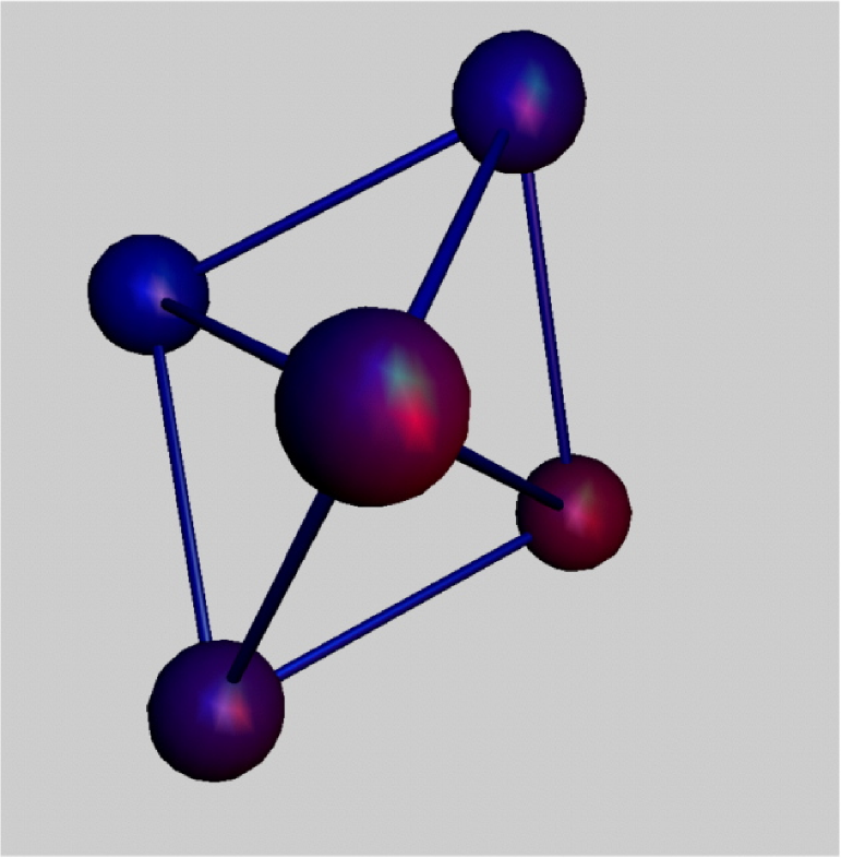
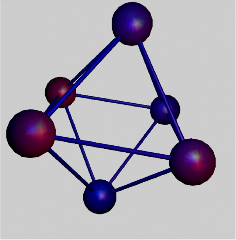
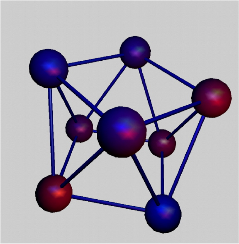
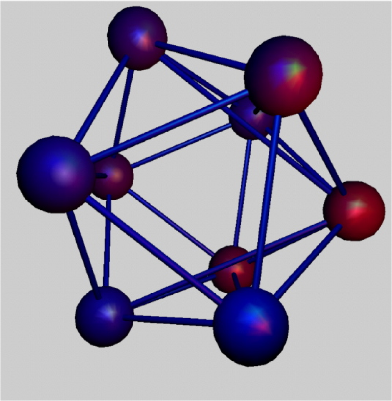
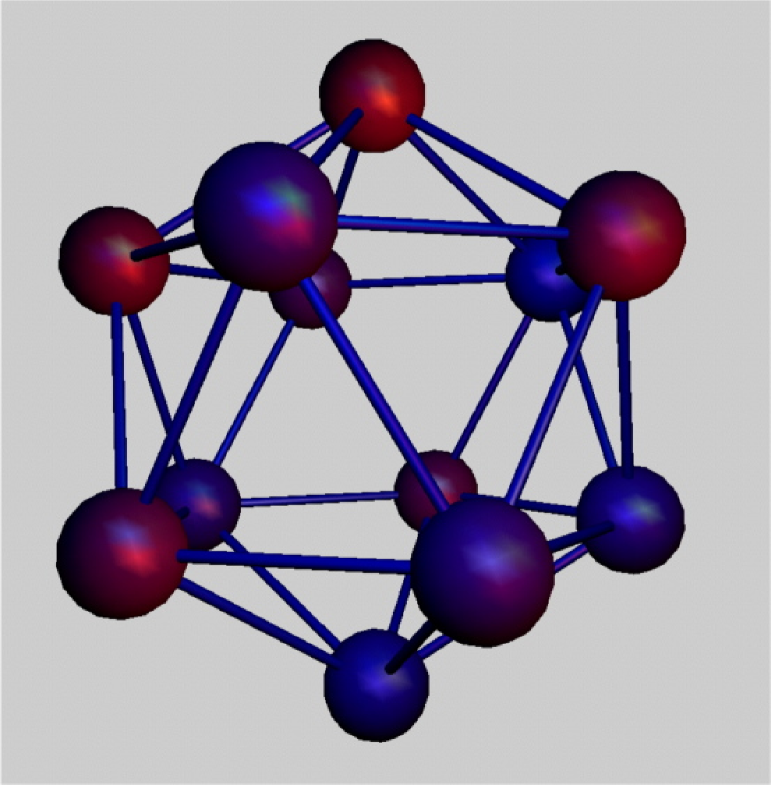
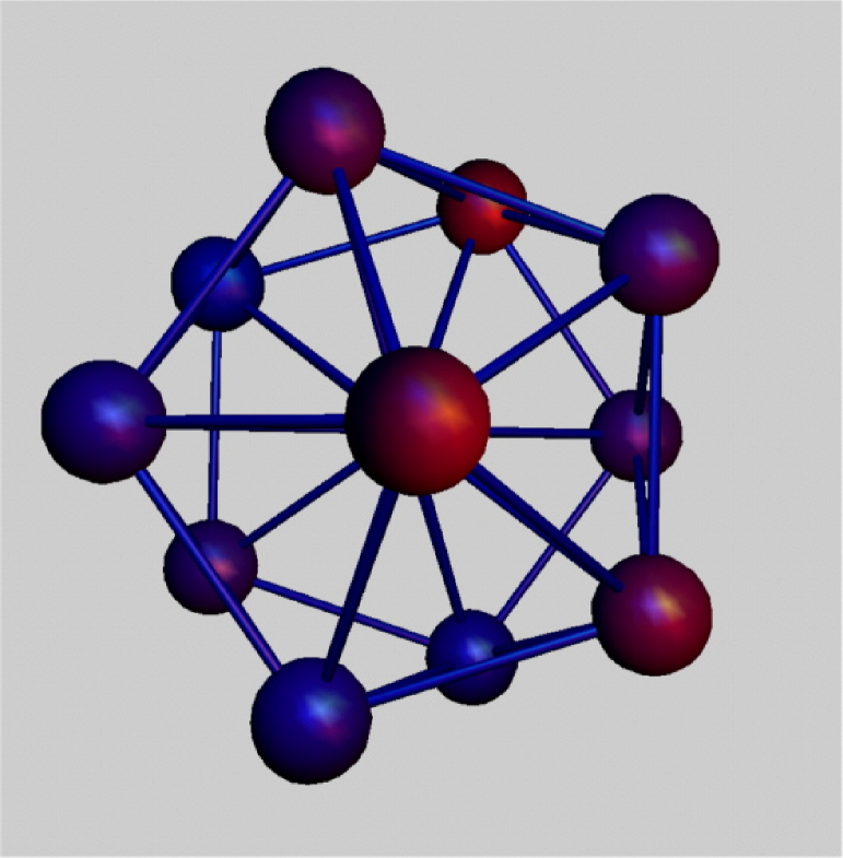
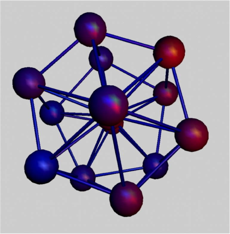
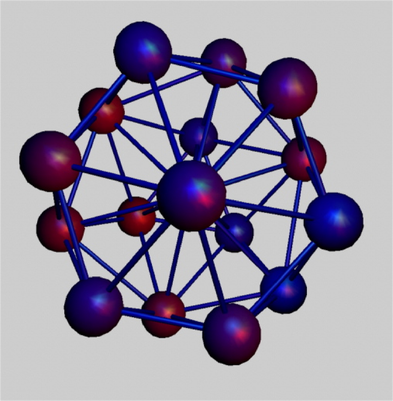
Figure 1: (Color online) A small set of remarkable equilibria for low $N$; from left to right and top to bottom: $N=$ [5] two tetrahedra joined at their bases, [6] two pyramids joined at their bases, [8] a twisted cube (three pyramids each pair sharing a base edge), [12] Icosahedron i.e. two skewed pentagonal pyramid, [13] Icosahedron+center, [14] hexagonal+ pentagonal pyramids+center, [17] hexagonal pyramid over hexagon over triangle+center, [18] two pentagonal pyramids+twisted pentagon center. Java animations describing theses oscillating crystals are found at http://www.iap.fr/users/pichon/nbody.html.

We consider $N$ particles of masses $m_{i}$ at ${\bf r}_{i},~{}i=N$ and set

$$\sum m_{i}=M,~{}\quad\sum m_{i}{\bf r}_{i}=M\overline{\bf r}\,,$$ (1)

and half the trace of the intertial tensor as

$$I=\sum m_{i}({\mathbf{r}}_{i}-\overline{\bf r})^{2}\equiv{M}a^{2},$$ (2)

which defines the scale $a$. In earlier work we showed both classically (paper I) and quantum mechanically Lynden-Bell & Lynden-Bell, (1999b) (paper II) that if the potential energy of the whole system was of the form

$$V=W(a)+a^{-2}W_{2}(\hat{\bf a})\,,$$ (3)

where $\hat{\bf a}$ is the 3N dimensional unit vector

$$\hat{\bf a}=\frac{N^{-1/2}}{a}({\bf r}_{1}-\overline{\bf r},~{}{\bf r}_{2}-\overline{\bf r}~{}....~{},~{}{{\bf r}}_{N}-\overline{\bf r})\,,$$ (4)

then the motion of the scaling variable $a$ separates dynamically from the motions of both $\overline{\bf r}$ and the $\hat{\bf r}$ so those motions decouple. If we ask that $V$ be made up of a sum of pairwise interactions then the hyperspherical potential, $W$, (independent of direction in the $3N-3$ dimensional space) has to be of the form:

$$W(a)=\frac{1}{2}\omega^{2}Ma^{2}=V_{-2}\,,$$ (5)

where $\omega^{2}$ is constant but depends linearly on $M$, and

$$W_{2}(\hat{\bf a})=a^{2}V_{2}=a^{2}\sum\sum\limits_{i<j}K_{2}|r_{i}-r_{j}|^{-2}\,.$$ (6)

Hence $W_{2}$ is a function of $\hat{\bf a}$ and is independent of the scale $a$.

II.1.1 Relationship to the Virial Theorem

Let us now see why potentials of the for $V_{2}+V_{-2}$ are so special by looking at the Virial Theorem and the condition of Energy conservation. Take the more general potential energy to be a sum of pieces $V_{n}$ where each $V_{n}$ scales as $r^{-n}$ on a uniform expansion. $n$ can be positive or negative. Then $V=\sum V_{n}$. For such a system the Virial Theorem reads:

$$\frac{1}{2}\ddot{I}=2T+\sum nV_{n}=2E+\sum(n-2)V_{n}~{}.$$

Now we already saw that $V_{-2}\propto I$ and $V_{2}$ clearly drops out of the final sum because $n-2$ is zero. Thus for potentials of the form $V=V_{-2}+V_{2}$

$$\frac{1}{2}\ddot{I}=2E-4V_{-2}=2E-4\omega^{2}\left(\frac{1}{2}I\right)\,,$$ (7)

so $I$ vibrates harmonically with angular frequency $2\omega$ about a mean value $E/\omega^{2}$ and shows no Violent Relaxation (1). Multiplying by $4\dot{I}$ and integrating

$$\dot{I}^{2}=8EI-4\omega^{2}I^{2}-4{M}^{2}\mathcal{L}^{2}\,,$$

where the last term is the constant of integration chosen in conformity with Eq. (8). Now recall from Eq. (2) that $I={M}a^{2}$ so we find on division by $8M^{2}a^{2}$ that

$$\frac{\dot{a}^{2}}{2}+\frac{\mathcal{L}^{2}}{2a^{2}}+\frac{1}{2}\omega^{2}a^{2}=\frac{E}{M}\,,$$ (8)

which we recognise as the specific energy of a particle with specific “angular momentum” $\mathcal{L}$ moving in a simple harmonic spherical potential of ‘frequency’ $\omega$. In such a potential $a$ vibrates about its mean at ‘frequency’ $2\omega$.

Note here that the $\gamma=5/3$ fluid also has a term $3(\gamma-1)U=2U$ in the virial theorem since its internal energy, $U$, scales like $r^{-2}$ so it can be likewise absorbed into the total energy term. Thus if every elementary mass of such a fluid attracted every other with a force linearly proportional to their separation, then that system too would pulsate eternally, as described above in Eq. (7) (see Section II.2 below).

The aim of this paper is to demonstrate the existence of perpetually pulsating equilibrium lattices and to study the changes as the non-pulsational ‘energy’ ${M}\mathcal{L}^{2}/2$ is increased. We show that the part of the potential left in the equation of motion for the rescaled variables is the purely repulsive $V_{2}$. It is then not surprising that the lattice disruption at higher non-pulsational energy occurs quite smoothly and the solid phase appears to give way to the “gaseous” phase of half the specific heat without the appearance of a liquid with another phase transition. The hard sphere solid has been well studied and behaves rather similarly.

Figure 2: (Color online) An example of large $N$ static spherical equilibrium obeying Eq. (9); here only a given shell is represented for clarity.

II.1.2 The Equations of Motion and their separation

Although the work of this section can be carried out when the masses $m_{i}$ are different, (see paper I), we here save writing by taking $m_{i}=m$ and so $M=Nm$. We start with $V$ of the form (3). The equations of motion are

$$m\ddot{\bf r}_{i}=-\partial V/\partial{\bf r}_{i}~{}~{}.$$ (9)

Now $V$ is a mutual potential energy involving only ${\bf r}_{i}-{\bf r}_{j}$ so $\sum\limits_{i}\partial V/\partial{\bf r}_{i}=0$ and summing the above equation for all $i$ we have

$$d^{2}\overline{\bf r}/dt^{2}=0~{}~{}~{},~{}~{}~{}\overline{\bf r}=\overline{\bf r}_{0}+{\bf u}t~{}~{}.$$

Henceforth we shall remove the centre of mass motion and fix the centre of mass at the origin so $\overline{\bf r}=0$. Now the $3N$-vector ${\bf a}$ can be rewritten in terms of its length $a$ and its direction $\hat{\bf a}\equiv{\bf a}/a$ (a unit vector). Equation (9) takes the form

$$M\ddot{\bf a}=-\partial V/\partial{\bf a}=-W^{\prime}\hat{\bf a}+2a^{-3}W_{2}\hat{\bf a}-a^{-3}\partial W_{2}/\partial\hat{\bf a}\,,$$ (10)

where we have used the form (3) for $V$. Notice that when $W_{2}$ is zero (or negligibly weak) all the hyperangular momenta of the form $m(r_{\alpha}\dot{r}_{\beta}-r_{\beta}\dot{r}_{\alpha})$ where $\alpha\neq\beta$ run from 1 to $3N$, are conserved!

Taking the dot product of (10) with ${\bf a}$ eliminates the $\partial W_{2}/\partial\hat{\bf a}$ term which is purely transverse so we get the Virial Theorem in the form:

$$\frac{1}{2}\frac{{{\mathrm{d}}}{}^{2}}{{{\mathrm{d}}}t^{2}}(Ma^{2})=M\dot{\bf a}^{2}-a\frac{{{\mathrm{d}}}W}{{{\mathrm{d}}}a}-\frac{2}{a^{2}}W_{2}=2E-\frac{1}{a}\frac{{{\mathrm{d}}}}{{{\mathrm{d}}}a}(a^{2}W)~{}.$$ (11)

Multiplying by ${{{\mathrm{d}}}(a^{2})}/{{{\mathrm{d}}}t}/2$ and integrating Eq. (11) yields

$$\frac{1}{2}Ma^{2}\dot{a}^{2}=Ea^{2}-Wa^{2}-\frac{1}{2}M\mathcal{L}^{2}\,,$$

where the final term is the constant of integration. On division by $a^{2}$

$$\frac{M}{2}\left({\dot{a}^{2}}+\frac{{\mathcal{L}}^{2}}{a^{2}}\right)+W(a)=E\,,$$ (12)

which is the energy equation of a particle of mass $M$ moving with angular momentum $\mathcal{L}$ and energy $E$ in a hyperspherical potential $W(a)$. Now

$$\ddot{\bf a}=\frac{{{\mathrm{d}}}{}}{{{\mathrm{d}}}t}(\dot{a}\hat{\bf a}+{a}\dot{\bf\hat{a}})=\ddot{a}\hat{\bf a}+\frac{1}{a}\frac{{{\mathrm{d}}}{}}{{{\mathrm{d}}}t}(a^{2}\dot{\bf\hat{a}})\,$$ (13)

and from (12)

$$\ddot{a}=\frac{\mathcal{L}^{2}}{a^{3}}-\frac{1}{M}W^{\prime}(a)~{}~{}.$$ (14)

Inserting these values for $\ddot{\bf a}$ and $\ddot{a}$ into equation (10) we obtain on simplification, multiplying by $a^{3}$:

$$Ma^{2}\frac{{{\mathrm{d}}}{}}{{{\mathrm{d}}}t}\left(a^{2}\frac{{{\mathrm{d}}}\hat{\bf a}}{{{\mathrm{d}}}t}\right)=2W_{2}\hat{\bf a}-\partial W_{2}/\partial\hat{\bf a}-M\mathcal{L}^{2}\hat{\bf a}~{}~{}.$$ (15)

On writing ${{\mathrm{d}}}{}/{{\mathrm{d}}}\tau=a^{2}{{\mathrm{d}}}{}/{{\mathrm{d}}}t$ this becomes an autonomous equation for $\hat{\bf a}(\tau)$. Since $(\dot{\bf a})^{2}=(a\dot{\hat{\bf a}}+\dot{a}\hat{\bf a})^{2}=a^{2}\dot{\hat{\bf a}}^{2}+\dot{a}^{2}$ we may write the energy in the form

$$E=\frac{1}{2}M\left[\frac{1}{a^{2}}\left(\frac{d\hat{\bf a}}{d\tau}\right)^{2}+\dot{a}^{2}\right]+V=\frac{1}{2}M\left(\dot{a}^{2}+\frac{\mathcal{L}^{2}}{a^{2}}\right)+W\,,$$

so

$$\frac{1}{2}M\left(\frac{{{\mathrm{d}}}\hat{\bf a}}{{{\mathrm{d}}}\tau}\right)^{2}+W_{2}=\frac{1}{2}M\mathcal{L}^{2}~{}~{}.$$ (16)

This shows that the only ‘potential’ in the hyper angular coordinates’ motion is $W_{2}(\hat{\bf a})$ and that the effective hyper angular energy in that motion is $\frac{1}{2}M\mathcal{L}^{2}$ (which has the dimension of $a^{2}$ times an energy). In fact we showed in papers I and III that it was this quantity that was equally shared among the hyperangular momenta in the statistical mechanics of perpetually pulsating systems. (15) gives the equation of motion for $\hat{\bf a}$. In terms of the true velocities ${\bf v}_{1},~{}{\bf v}_{2}$ etc

$$\frac{{{\mathrm{d}}}\hat{\bf a}}{{{\mathrm{d}}}\tau}=\sqrt{N}\!a^{2}\frac{{{\mathrm{d}}}{}}{{{\mathrm{d}}}t}\left(\frac{{\bf r}_{1}}{a},~{}\frac{{\bf r}_{2}}{a}~{}....~{}\frac{{\bf r}_{N}}{a}\right)=$$

$$a\left({\bf v}_{1}-\frac{\dot{a}}{a}{\bf r}_{1},{\bf v}_{2}-\frac{\dot{a}}{a}{\bf r}_{2}~{}...~{}{\rm\sl etc}\right)\,,$$

so it is the peculiar velocities after removal of the Hubble flow ${\dot{a}}{\bf r}_{i}/{a}$ and after multiplication by $a$ that constitute the kinetic components of the shared angular energy in the angular potential $W_{2}(\hat{\bf a})$.

When the $m({{\mathrm{d}}}\hat{\bf a}/{{\mathrm{d}}}\tau)^{2}/2$ are large enough to escape the potential wells offered by $W_{2}/N$ we get an almost free particle angular motion of these $3N-4$ components. The $-4$ accounts for the fixing of the centre of mass and the removal of $\dot{a}$ from the kinetic components. If we impose also a prescribed total angular momentum, the number of independent kinetic components would reduce by a further three components to $3N-7$. However the peculiar velocities are then measured relative to a frame rotating with angular velocity ${\bf\Omega}$ where ${\bf\Omega}={\bf\cal I}^{-1}\cdot{\bf J}$ where ${\mathbf{J}}$ is the angular momentum of the system. Here $\cal I$ is the inertial tensor, not to be confused with $I={\rm trace}({\cal I})/2$ introduced in Section II.1.1. The constant Lagrange multiplier is no longer ${\bf\Omega}$, which is proportional to $a^{-2}$ since the inertial tensor, has that dependence in pulsating equilibria. The Lagrange multiplier is ${\tilde{\bf J}}={\bf\Omega}a^{2}$ which is constant during the pulsation and the peculiar velocity is ${\bf v}_{\rm pi}=({\bf v}_{i}-{\bf u}_{i})$ where ${\bf u}_{i}=\left({\dot{a}}{\bf r}_{i}/{a}+{\tilde{\bf J}}\times{\bf r}_{i}/{a^{2}}\right)$ see paper III equation (17). Hereafter we specialise to the requirements given by Eq. (5) and  (6).

II.2 The $\gamma=5/3$ analogous fluid system

When particles attract with both a long range force such as gravity or our linear law of attraction, and a short rage repulsion, the latter acts like the pressure of a fluid. Indeed short range repulsion forces only extend over a local region, and for large $N$ their effect can be considered as pressure since only the particles close to any surface drawn through the configuration affect the exchange of momentum across that surface. In our case, the local $r_{ij}^{-3}$ forces come from the $r_{ij}^{-2}$ potential which scales as $r^{-2}$. A barotropic fluid with $p=\rho^{\gamma}$ has an internal energy that behaves as $\rho^{\gamma-1}$ scaling like $r^{-3(\gamma-1)}$. The required $r^{-2}$ scaling gives a $\gamma$ of $5/3$, i.e. a polytropic index of $n=3/2$, the same as a non relativistic degenerate white dwarf. Thus we may expect analogies between a $\gamma=5/3$ fluid with the linear long range attraction, and our large $N$ particle systems. However an $r_{ij}^{-3}$ repulsion between particles is not of very short range so this fluid is not the same as the large $N$ limit of the particle system. The particle equilibria have the inverse cubic repulsion between particles balancing the long range linear attraction, which can be exactly replaced by a linear attraction to the barycentre proportional to the total mass. For the fluid, it is the pressure gradient that balances this long range force.

II.2.1 Mass profile of the static polytropic fluid

The equilibrium of such a fluid in the presence of a long range force, $-G^{\star}Mr$, (where $MG^{\star}\equiv\omega^{2}$) is given by

$$\frac{1}{\rho}\frac{{{\mathrm{d}}}p}{{{\mathrm{d}}}r}=-G^{\star}Mr\,.$$ (17)

Setting $p=\kappa\rho^{5/3}$, with $\xi\equiv r/r_{\rm m}$, this yields

$$\rho=\rho_{0}(1-\xi^{2})^{{3/2}},$$ (18)

where ${\mathbf{r}}$ is the 3D configuration space vector measured from the centre of mass of the system and $r$ its modulus, with $r_{\rm m}$ its value at the edge.

Integrating the density gives a mass profile, $M(\xi)$,

$$M(\xi)=\frac{2M}{3\pi}\left(3\arcsin(\xi)-\xi(8\xi^{4}-14\xi^{2}+3)\sqrt{1-\xi^{2}}\right),$$ (19)

and $M$ is the total mass. In practice for the discrete system of Section II.1, there is a marked layering at equilibrium, and the “pressure” and the mass profiles depart from their predicted profiles as each monolayer of particles is crossed. See Section III and Fig. (3).

The relationship between the polytropic coefficient, $\kappa$, and $K_{2}$, the strength of the repulsion (entering $W_{2}$ in Eq. (6)) is found by identifying the internal energy of the corresponding fluid to the potential energy of the $1/r_{ij}^{2}$ coupling. In short, the former reads for a $\gamma=5/3$ fluid with density profile Eq. (17):

$$V_{2}=-\int_{0}^{r_{\rm m}}\frac{\kappa\gamma}{\gamma-1}\rho^{2/3}4\pi r^{2}\rho{{\mathrm{d}}}r=-\frac{25\pi^{2}}{128}\kappa\rho_{0}^{5/3}r_{\rm m}^{3}\,,$$ (20)

while the latter reads:

$$-\frac{K_{2}}{2}\int\!\!\!\!\!\int\!\!\!\!\!\int_{0}^{r_{\rm m}}\!\!\frac{8\pi r^{2}\rho(r)\pi r^{{}^{\prime}2}\rho(r^{\prime}){{\mathrm{d}}}\mu\,{{\mathrm{d}}}r\,{{\mathrm{d}}}r^{\prime}}{r^{2}+r^{{}^{\prime}2}-2\mu\,r\,r^{\prime}}=-\frac{9\pi^{4}}{320}\rho_{0}^{2}r_{\rm m}^{4}K_{2}\,.$$ (21)

Identifying Eq. (20) and  (21) gives (using $M=\pi^{2}\,\rho_{0}r_{\rm m}^{3}/8$ consistant with the density profile, Eq. (18))

$$\kappa=\frac{36}{125}\pi^{4/3}M^{1/3}K_{2}.$$ (22)

Similarly, requiring that $V_{2}$ and $V_{-2}$ balance at static equilibrium, where

$$V_{-2}=\int\rho(r)\,\frac{\omega^{2}\,r^{2}}{2}4\pi r^{2}{{\mathrm{d}}}r=\frac{3\pi^{2}}{128}\omega^{2}\rho_{0}r_{\rm m}^{5}\,,$$ (23)

yields

$$\rho_{0}=\left(\frac{5G^{\star}}{3K_{2}}\right)^{3/4}\,\frac{M}{\pi^{2}}\,,\quad{\rm and}$$ (24)

$$r_{\rm m}=2\left(\frac{3K_{2}}{5G^{\star}}\right)^{1/4}\,\,.$$ (25)

Eqs. (18)-(25) allow us to relate the properties of the crystal to the properties of the analogous fluid system. Notice that $r_{\rm m}$ is independent of $M$ and $\rho_{0}$ is proportional to $M$.

II.2.2 Figure of rotating configurations

Equilibrium in the rotating frame with the angular rate, ${\mathbf{\Omega}}$ (not to be confused with $\omega$, the strength of the harmonic potential introduced in Eq. (5)), requires that:

$$\frac{1}{\rho}\nabla p=\nabla(\psi+\frac{1}{2}\Omega^{2}R^{2})\,,\quad{\rm where}\quad\psi=-\frac{1}{2}G^{\star}M\textsf{r}^{2}\,,$$ (26)

where $R$ is the distance off axis ($r^{2}=R^{2}+z^{2}$). Since $p=\kappa\rho^{5/3}$, it follows that, with $\Omega_{\star}^{2}=\Omega^{2}/(G^{\star}M)$,

$$\frac{5}{2}\kappa\rho^{2/3}=-\frac{G^{\star}M}{2}(z^{2}+(1-\Omega_{\star}^{2})R^{2})+{\rm const.}$$ (27)

Let $\rho=0$ at $z=z_{0}$ on axis, then

$$\frac{\rho}{\rho_{0}}=\left(1-\frac{z^{2}}{z_{0}^{2}}-(1-\Omega_{\star}^{2})\frac{R^{2}}{z_{0}^{2}}\right)^{3/2}.$$ (28)

From this we can derive the mass, $M$ and the moment of inertia, ${\cal I}$ as functions of the $z_{0}$, $\rho_{0}$

$$M=\frac{\pi^{2}}{8}\frac{\rho_{0}z_{0}^{3}}{1-\Omega_{\star}^{2}}\,,\quad{\rm and\quad{\cal I}=\frac{1}{4}MR_{0}^{2}}\,,$$ (29)

where $R^{2}_{0}=z^{2}_{0}/(1-\Omega_{\star}^{2})$ and $z_{0}^{2}=5\kappa/\rho_{0}^{2/3}/\mathcal{L}^{2}$. Eq. (28) generalizes Eq. (18) when the $\gamma=5/3$ fluid is given some angular momentum. The ellipticity, $\varepsilon$, of the rotating configuration is given by

$$\varepsilon^{2}=1/(1-\Omega_{\star}^{2})=1/(1-\Omega^{2}/\omega^{2})\,.$$ (30)

Fig. (6) displays the corresponding configuration for $N=64$.

II.2.3 Dynamics of the rotating oscillating $\gamma=5/3$ fluid

The basic pulsation of the $\gamma=5/3$ fluid in rotation is given by a time dependent uniform expansion/contraction plus a rotation at constant angular momentum. Thus

$${\mathbf{u}}=\frac{\dot{a}}{a}{\mathbf{r}}+\frac{1}{a^{2}}{\tilde{\mathbf{J}}}\times{\mathbf{r}}\,,$$ (31)

where $a(t)$ is the “expansion factor” of Section II.1 and ${\tilde{\mathbf{J}}}$ is the constant Lagrange multiplier associated with angular momentum conservation. The acceleration involved in this motion are

$$\frac{{\rm D}{\mathbf{u}}}{{\rm D}t}=\frac{\partial{\mathbf{u}}}{\partial t}+{\mathbf{u}}\cdot\nabla{\mathbf{u}}=\frac{\partial{\mathbf{u}}}{\partial t}+\nabla\left(\frac{1}{2}{\mathbf{u}}^{2}\right)-{\mathbf{u}}\times(\nabla\times{\mathbf{u}})\,.$$ (32)

Given that $\nabla\times{\mathbf{u}}=2{\tilde{\mathbf{J}}}/a^{2}$, putting Eq. (31) into  (32) yields

$$\frac{{\rm D}{\mathbf{u}}}{{\rm D}t}=\nabla\left(\frac{\ddot{a}}{a}\frac{r^{2}}{2}-\frac{1}{2a^{4}}({\tilde{\mathbf{J}}}\times{\mathbf{r}})^{2}\right)\,.$$ (33)

Differentiating Eq. (8) yields:

$$\ddot{a}=\frac{{\cal L}^{2}}{a^{3}}-\omega^{2}a\,,$$ (34)

while Euler’s equation reads:

$$\frac{{\rm D}{\mathbf{u}}}{{\rm D}t}=-\nabla\left(\frac{5}{2}\kappa\rho^{2/3}+\frac{1}{2}\omega^{2}r^{2}\right)\,.$$ (35)

Equating Eq. (35) and  (33) together with Eq. (34) yields:

$${\nabla}\left(\frac{5}{2}\kappa{\rho}^{2/3}+\frac{1}{2a^{4}}{\cal L}^{2}{r}^{2}-\frac{1}{2a^{4}}\left({\tilde{\mathbf{J}}}\times{\mathbf{r}}\right)^{2}\right)=0\,.$$ (36)

Now in the rescaled space, $\rho\equiv{\tilde{\rho}}/a^{3}$, ${\mathbf{r}}\equiv{\tilde{\mathbf{r}}}a$ and $\nabla\equiv{\tilde{\nabla}}/a$, Eq. (36) reads

$${\tilde{\nabla}}\left(\frac{5}{2}\kappa\tilde{\rho}^{2/3}+\frac{1}{2}{\cal L}^{2}{\tilde{r}}^{2}-\frac{1}{2}\left({\tilde{\mathbf{J}}}\times{\mathbf{\tilde{r}}}\right)^{2}\right)=0\,.$$ (37)

which is the equilibrium condition but with the time-dependently rescaled variables replacing the original ones. Hence it follows that in the comoving rotating frame, the $\gamma=5/3$ fluid will stratify in the same manner as Eq. (28) but in the rescaled variables (${\tilde{R}_{0}}^{2}={\tilde{z}_{0}}^{2}/(1-{\tilde{J}}^{2}/\mathcal{L}^{2})$ and ${\tilde{z}}_{0}^{2}=5\kappa/{\tilde{\rho}}_{0}^{2/3}/\mathcal{L}^{2}$). This maintains a constant ellipticity during the oscillation, since ${\tilde{R}_{0}}$ and ${\tilde{z}_{0}}$ are independent of $a(t)$.

III Applications: crystalline forms of pulsating equilibria

Let us now study the discrete form of rotating pulsating equilibria that the systems described in Section II follow. Let us first ask ourselves what would the final state of equilibrium in which $N$ particles obeying Eq. (9) would collapse to, if one adds a small drag force in order to damp the motions.

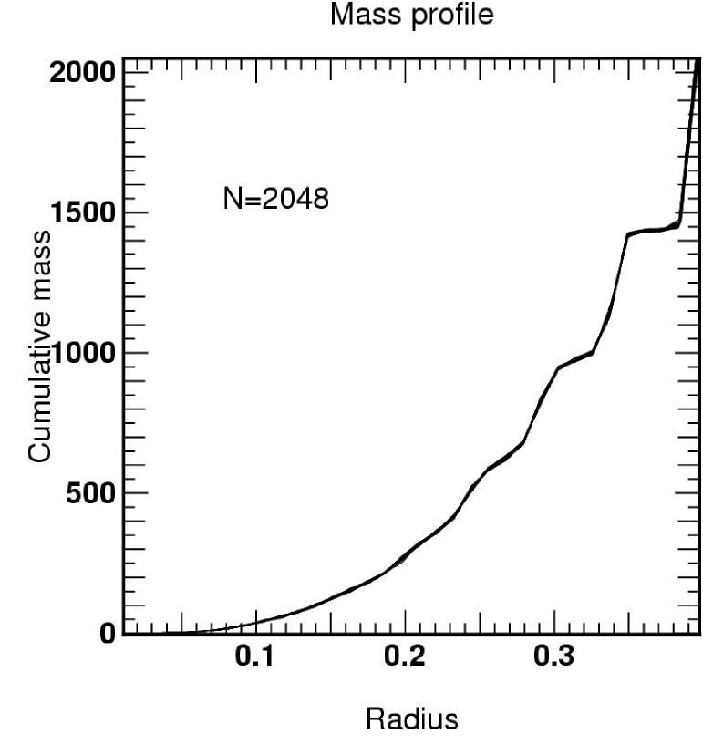
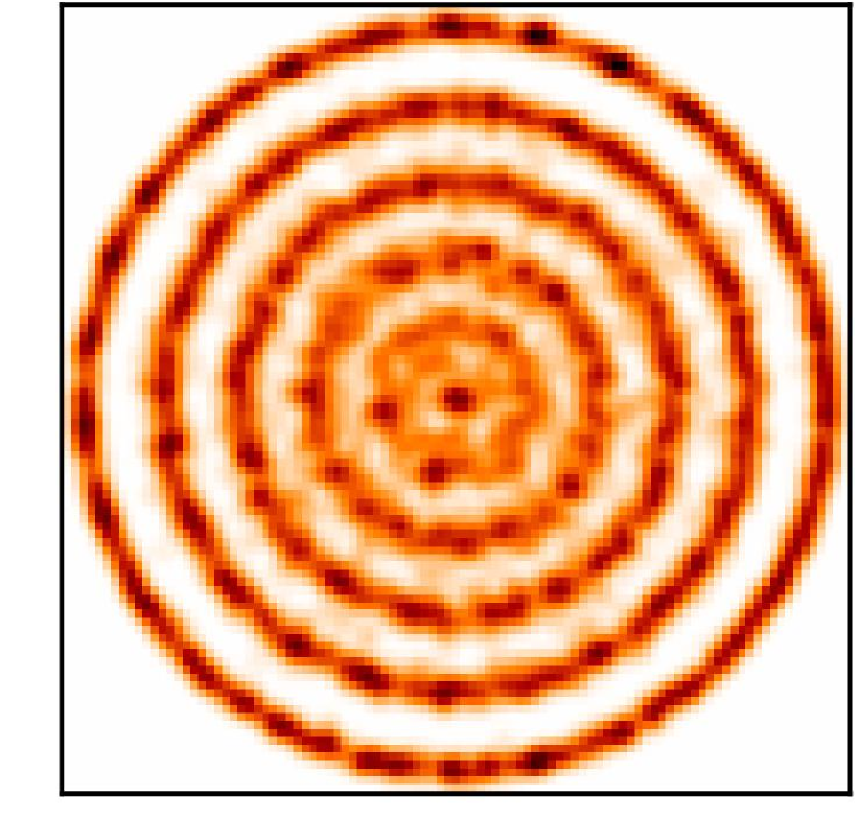
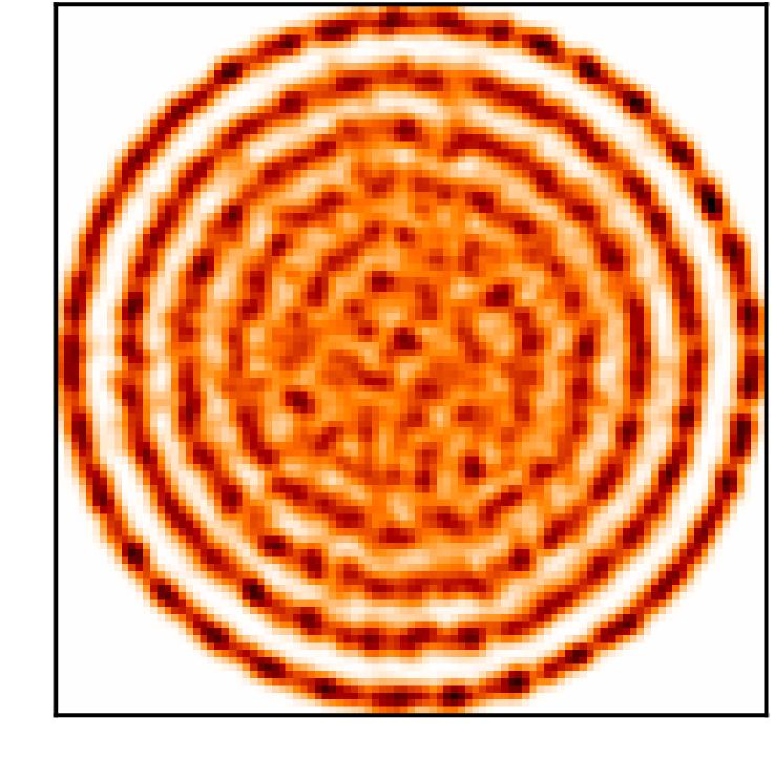
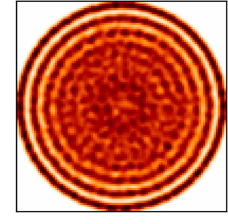
Figure 3: top: (Color online) Mean mass profile and section (top) though a $N=512$, $N=1024$ and $N=2048$ crystal; The mass profile is derived while stacking about 20 realisations of the lattice and binning the corresponding density. The shell structure (bottom) is clearly apparent on these sections. The number of shell, $N$, present is consistent with the prediction of Section III.1.2. The ordering of the inner regions is lower as $N$ increases since the inner shells do not settle gently as they are disturbed by the infall of the outer layers.

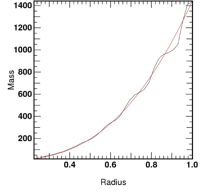
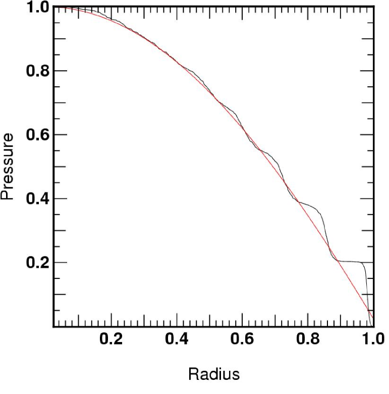
Figure 4: (Color online) Mass profile and Pressure of an $N=2048$ simulation together with a fit of its analytic prediction given by Eq. (18) and  (19) (see Section III.1.4 and Fig. (5) for a discussion of the accuracy of this fit). The mass profile is computed via the cumulative number of particles within a given shell, while the pressure profile is estimated via Eq. (39).

Numerical setup

A softening scale, $s$, of $0.05$ was used so that The effective interaction potential reads

$$\psi_{12}=G^{\star}\frac{r_{12}^{2}}{2}+\frac{K_{2}}{r_{12}^{2}+s^{2}}\,.$$ (38)

We may escale both the repulsive, $K_{2}$ and the attractive strength, $G^{\star}$ of the potential to one by choosing appropriately the time units and the scale units. As a check, we compute the total energy of the cluster, together with the invariant, $m{\cal L}^{2}/2$ and check its conservation.

III.1 Static Equilibrium

The relaxation towards the equilibrium should be relatively smooth in order to allow the system to collapse into a state of minimal energy. We will consider here two different damping forces; first (in Section III.1) an isotropic force, proportional to $-\alpha{\mathbf{v}}$ so that both the rotation and the radial oscillations are damped; or, in Section III.2.1, a drag force so that the components of the velocity are damped until centrifugal equilibrium is reached.

III.1.1 Few particle Equilibria

Figure 1 displays the first few static equilibria, while Table 1 lists the first 18, which includes in particular the regular Icosahedron for $N=12$. Strikingly, roughly beyond this limit of about $N=20$, there exists more than one set of equilibria for a given value of $N$, and the configuration of lowest energy is not necessarily the most symmetric. The overall structure is not far from hexagonal close packed, but with a spherical layering at large radii. Java animations describing the crystals are found at http://www.iap.fr/users/pichon/nbody.html.

III.1.2 Larger N limit

Figure 3 displays both the mean mass profile and the corresponding section though $512\leq N\leq 2048$ lattices; both the mass profile and the sections are derived while stacking different realisations of the lattice and binning the corresponding density. Note that the inner regions are more blurry as $N$ increases; indeed, the inner layers are frozen early on by the infall of the outer layers.

Let us estimate the pressure profile in our crystal. In static equilibrium, given Eq. (17), we should have approximately

$$p(r)=\int\omega^{2}\rho(r)r{{\mathrm{d}}}r=\frac{\omega^{2}}{4\pi}\int_{r}^{r_{\rm m}}\frac{{{\mathrm{d}}}m}{r}\approx\frac{\omega^{2}}{4\pi}\sum_{r^{\prime}>r}\frac{m}{r^{\prime}}\,.$$ (39)

Eq. (39) is compared to Eq. (17) in Fig. (4).

III.1.3 Mean density profile

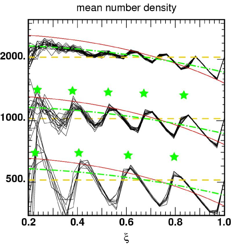
Figure 5: (Color online) shows the mean number density profile, $N\,{\bar{n}}(\xi)$ for a set of about 10 $N=512$, $1024$ and $2048$ simulations as a function of rescaled radius. The wiggles correspond to the shells seen in Fig. (3). The thin line corresponds to the prediction of Eq. (19) for the fluid system, but with an outer radius rescaled by the predicted radius, Eq. (25) divided by the measured outer radius, $r_{\rm m}$; the dashed line corresponds to a uniform density solid, while the dotted dashed line corresponds to the prediction of Eq. (42) (rescaled, see text). Clearly, this last model gives the best fit to the mean profile, which suggests that for those values of $N$, the crystal does behave according to the equilibrium Eq. (40), and neither like a pure solid nor as a fluid. The stars correspond to the predictions of the shell radii given by Eq. (43).

Fig. (5) shows the mean density within rescaled radius, $\xi=r/r_{\rm m}$ as a function of $\xi$ for three different simulations. The shell structure is very obvious but at larger $N$ values it is also clear that besides the oscillations due to shells the mean density falls off somewhat towards the outside. However such a fall off is far less pronounced than that predicted by the polytropic model which gave ${\bar{\rho}}(\xi)=M(\xi)/(4\pi r_{\rm m}^{3}\xi^{3/3})$ with $M(\xi)$ given by Eq. (19). On further inspection, it transpired that this is due to the longer range of the repulsion force which is not correctly represented by the pressure analogy.

Consider a continuum density distribution with a repulsive force between elements ${{\mathrm{d}}}{m}$ and ${{\mathrm{d}}}{\bar{m}}$ derived from the potential $K_{2}{{\mathrm{d}}}{m}{{\mathrm{d}}}{\bar{m}}/|{\mathbf{r}}-{\bar{\mathbf{r}}}|^{2}$. Then, for a spherical density distribution, $\rho({\bar{r}})$, the total potential reads

$$\psi(r)=K_{2}\!\!\int\!\!\!\!\int\frac{2\pi{\bar{r}}^{2}\rho({\bar{r}}){{\mathrm{d}}}{\mu}{{\mathrm{d}}}{\bar{r}}}{r^{2}+{\bar{r}}^{2}-2\,r{\bar{r}}\mu}=2\pi K_{2}\!\!\int\frac{{\bar{r}}\rho({\bar{r}})}{r}\log\left|\frac{r+{\bar{r}}}{r-{\bar{r}}}\right|{{\mathrm{d}}}{\bar{r}}$$

The condition of equilibrium balances against the harmonic attraction yields

$$-\frac{{{\mathrm{d}}}\psi}{{{\mathrm{d}}}r}=G^{\star}Mr\,,\quad r\leq r_{\rm m}\,.$$ (40)

Note that all the mass, not just that inside radius $r$, contributes to the attraction for the linear law. Eq. (40) generates a linear integral equation for $\rho({\bar{r}})$. A numerical solution to Eq. (40) shows that the mean density distribution agrees well with the simulations, once the shell structure is smoothed out (see Fig. (5)). The solution to the integral equation is well approximated by

$$\rho(r)=\rho_{0}\left(1-\frac{r^{2}}{6r_{\rm m}^{2}}\right)^{3}\,,\mbox{ where $r\leq r_{\rm m}$ }\,,$$ (41)

and $0$ beyond. The corresponding mean density within $r$, $\bar{n}$, scaled to one at the centre, reads

$${\bar{n}}(\xi)=\frac{3}{\rho_{0}\xi^{3}}\!\int^{\xi}\!\!\rho(r_{\rm m}\xi)\xi^{2}{{\mathrm{d}}}{\xi}=\left(1-\frac{3\,\xi^{2}}{10}+\frac{\xi^{4}}{28}-\frac{\xi^{6}}{648}\right)\!,$$ (42)

with $\xi\equiv r/r_{\rm m}$, and $n(r)\equiv\rho(r)/m$, (see Fig. (5)) so that at $\xi=1$, ${\bar{n}}(1)\equiv X=16\,651/22\,680$. The simulations have been scaled so that $\xi$ is one at the outermost particle. That will not be at the point at which the theoretical smooth density falls to zero which we have called $\xi=1$ in our theoretical calculation. In practice this falls outside the last particle, hence we have to rescale the theory’s $\xi$ by a factor $f$ which is determined to make the theoretical mean density profile, $\bar{n}$, fit the profile of the simulations’ mean density. Once this scaling $f$ has been determined the predicted mean density is given in terms of the observed $\xi$ by the expression $X{\bar{n}}(f\xi)N/[4/3\pi(fr_{\rm m})^{3}]$.

III.1.4 Stratification in spherical shells

In atoms, the main gradient of the potential is towards the nucleus, so the shell structure is dominated by the inner shells which have large changes in energy. In our systems, the global potential gradient is proportional to $r$ so the largest potential differences are on the outside. As a consequence, the system adjusts itself so that the outermost shell is almost full, and the central region is no longer shell dominated. Instead of counting shells outwards from the middle as in atoms, it is best to count shells inwards from the outside where they are best defined. For shells which are numbered from the outside, given that ${{\mathrm{d}}}r/n^{-1/3}(r)$ is the fractional increase in layer number, we have (using Eq. (41))

$$\int_{r_{i}}^{1}\frac{{{\mathrm{d}}}r}{n(r)^{-1/3}}=\frac{n_{0}^{1/3}r_{\rm m}}{X}\left[1-\xi_{i}-\frac{1}{18}(1-\xi_{i}^{3})\right]=i\,,$$ (43)

with $n_{0}\equiv\rho_{0}/m=3N/(4\pi r_{\rm m}^{3})$. Conversely, the number of particles, $N(\leq i)$ within (and including) layer $i$ is given by

$$N(\leq i)=\frac{N}{X}\,\xi_{i}^{3}\!\left[1-\frac{3}{10}\xi_{i}^{2}+\frac{1}{28}\xi_{i}^{4}-\frac{1}{648}\xi_{i}^{6}\right].$$ (44)

Solving the implicit Eq. (43) for the relative radius $\xi_{i}$ of layer $i$ and putting it into Eq. (44) yields the number of particles within layer $i$ as a function its rank. The radii of the layers, $\xi_{i}r_{\rm m}$ follows from inverting Eq. (43) for $\xi_{i}$. Examples of such shells are shown in Fig. (2) and  (3), while the corresponding mass profile checked against Eq. (19) in Fig. (4). The number of shell present in Fig. (3) is consistent with the prediction of Eq. (44).

III.2 Rotating Perpetually Pulsating Equilibria

III.2.1 Rotating crystals

The rotating crystal is achieved in steps; first, for each particle in the lattice, we added a velocity kick so that ${\mathbf{v}}\rightarrow{\mathbf{v}}+{\mathbf{\Omega}}\times{\bf r}$. We then rescale the $z$ coordinate and the $v_{z}$ (as defined along the momentum direction) of each particule by a constant factor. The system has then the ability to redistribute it momentum along the oscillating particles. We then add a drag force proportional to $-\alpha\left({\mathbf{v}}-{\mathcal{I}}^{-1}\cdot{\tilde{\mathbf{J}}}\right)$, so that the components of the velocity are damped until centrifugal equilibrium is reached. This defines the rotating spheroid equilibrium. An example of such a configuration is shown in Fig. (6) for $N=64$. The properties of the corresponding analogous fluid system are described in Section II.2.2.

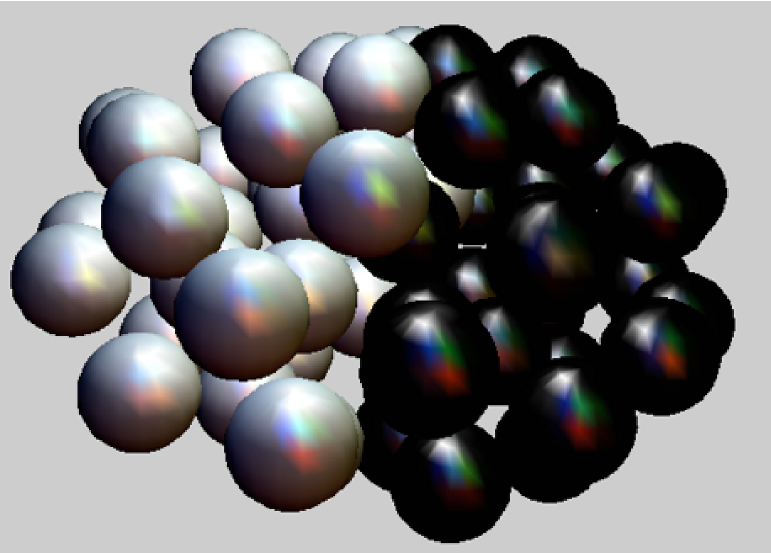
Figure 6: (Color online) spheroidal crystal corresponding to the final state of a run of $N=64$ with a damping force of the form $-\alpha\left({\mathbf{v}}-{\mathcal{I}}^{-1}\cdot{\tilde{\mathbf{J}}}\right)$. Half of the particles was painted one color, while the other half was left some other color. The shape preserving oscillation is achieved by rescaling all position by some factor, $\lambda$, and rescaling all velocities by the factor $1/\lambda$. If the rescaling does not preserve momentum of each particle, some of the excess energy may go into heating the system and breaking its structure, which will induce mixing of the two populations (see Section III.3.2 and paper III). Java animations corresponding to the corresponding oscillating rotating crystals are found at http://www.iap.fr/users/pichon/nbody.html.

III.2.2 Rotating pulsating crystals

In order to create a pulsating configuration which preserves the shape of the rotating spheroid, we rescaled all the positions by some factor, $\lambda$, and rescaled accordingly all velocities by the factor $1/\lambda$, so that angular momentum is preserved. When this special condition is met, the system oscillates and pulsates without any form of relaxation (cf. Section III.3). Note that this situation differs from normal modes of more classical systems, which do preserve the shape of a given oscillation, but might not involve the same particles at all times. Java animations describing the pulsating and rotating crystals are found at http://www.iap.fr/users/pichon/nbody.html.

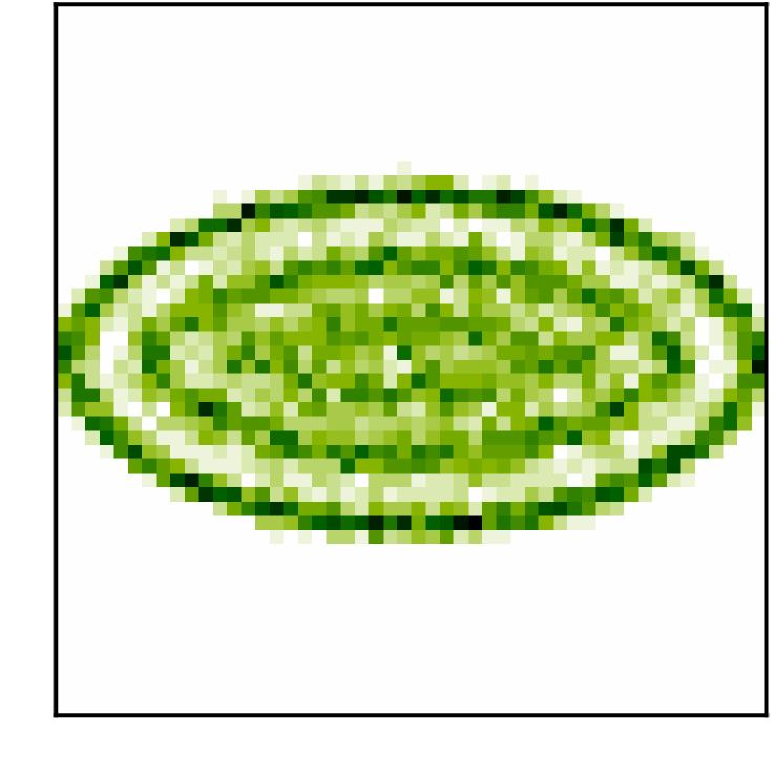
Figure 7: (Color online) Same as Fig. (3), but for a set of 20 rotating configuration of $N=256$ particles launched according to the prescription given in Section III.2.1. The shell structure is also clearly apparent on this section. The ellipticity of the crystal is found to be in agreement with Eq. (30).

III.3 Thermodynamics of dissolving crystal

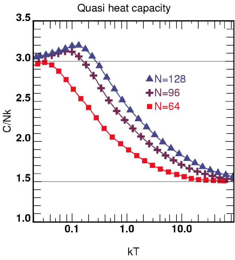
Figure 8: (Color online) quasi specific heat measured by increase of quasi energy with quasi temperature in units of $kN$; the quasi temperature is $a^{2}$ times the kinetic energy relative to the time dependent “Hubble flow” divided by $3/2\,Nk$; the quasi energy is the sum of the quasi kinetic energy plus $W_{2}$; $W_{2}$ is $a^{2}$ times the repulsive part of the potential energy. During the large amplitude pulsation of the system, the quasi energy is conserved. It is the quasi energy that is shared between the different components in the statistical equilibrium. Since $W_{2}$ is only repulsive, the system displays characteristics similar to a hard sphere fluid. There is a continuous transition between the cold crystal lattice and the “free” fluid. Each point is derived over a set of about 20 independent runs. The initial condition is set up with some random motions above the lattice equilibrium.

III.3.1 Specific heat & evaporation

How does the shell structure disappear as a function of temperature increase ? Fig. 8 displays the quasi-specific heat measured by the increase of quasi energy with quasi temperature in units of $kN$; Here the quasi temperature is $a^{2}$ times the kinetic energy relative to the time dependent “Hubble flow” divided by $3/2\,Nk$; while the quasi energy is the sum of the quasi kinetic energy plus $W_{2}$ given by Eq. (6). During the large amplitude pulsation of the system, the quasi energy is shared between the different components in the statistical equilibrium. Since $W_{2}$ is only repulsive, the system displays characteristics similar to a hard sphere fluid. The quasi-heat capacity changes from the solid’s $3Nk$ to the gaseous $3/2\,Nk$ as expected.

III.3.2 Relaxation of the rotating pulsating configuration

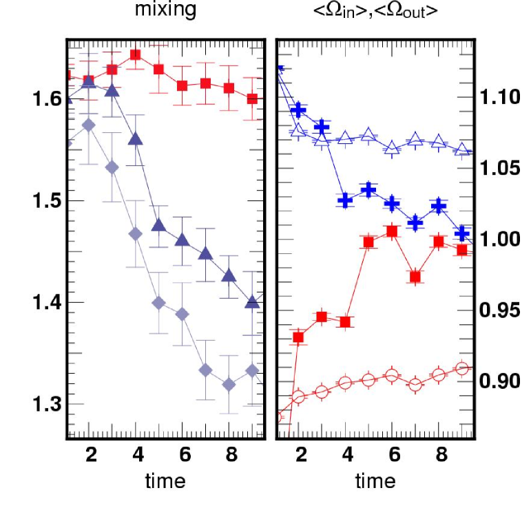
Figure 9: (Color online) left panel: $\Delta n_{\rm WB}/{\bar{n}_{\rm WB}}$, the relative dispersion in mixing as a function of time for a set of $N=64$ particles in a situation where the inner fraction of particles was rescaled along the rotation axis in order to induce some momentum exchange. Here three scalings (1.2, 1.6 and 2) were imposed (from top to bottom), corresponding to an increasing heat content which induce a faster relaxation. The initial condition corresponds to the prescription described in Section III.2.1 and Fig. (6). Right panel: $\Omega_{\rm in}(t)/{\bar{\Omega}}(t)$ and $\Omega_{\rm out}(t)/{\bar{\Omega}}(t)$ as a function of time; again the hotter initial configuration (rescaled by 1.8 compared to 1.2) (full symbol) reaches a regime of uniform rotation more rapidly.

Let us split the particles within our spheroidal equilibrium in two sets as a function of axial radius, $R$, one corresponding to an inner ring, and one corresponding to an outer ring (which should initially rotate at the same angular rate) and rescale the $z$ component of each inner particle by a factor of $2$ so that it does not satisfy the equilibrium condition.

A measure of the thermalisation is given by the rate at which the system will redistribute momentum in order to achieve uniform rotation again. Fig. (9) (right panel) represents $\Omega_{\rm in}(t)/{\bar{\Omega}}(t)$ and $\Omega_{\rm out}(t)/{\bar{\Omega}}(t)$ as a function of time (with ${\bar{\Omega}}(t)=[\Omega_{\rm in}(t)+\Omega_{\rm out}(t)]/2$).

III.3.3 Mixing of the rotating pulsating configuration

A measure of mixing is given by the rate at which the system becomes uniform, when it is started as two distinct phases. Let us start by a configuration where half of the particles on one side of the spheroidal rotating equilibrium are colored in WHITE, and the other half, in BLACK, and rescale again the coordinate along the rotation axis by a factor of two. The redistribution of the excess energy in height will convert a fraction of it into heat. Fig. (9) (left panel) represents $\Delta n_{\rm WB}/{\bar{n}_{\rm WB}}\equiv{\rm RMS}(n_{\rm B}(t)-n_{\rm W}(t))/{\rm RMS}(n_{\rm B}(t)+n_{\rm W}(t))$, with $n_{\rm R}$ the density of WHITE particles, and $n_{\rm B}$ the density of BLACK particles as a function of time. In practice, we bin the $x$–$y$ plane in the comoving coordinates and estimate $\Delta n_{\rm WB}/{\bar{n}_{\rm WB}}$ accordingly.

IV Conclusion

In this paper, we have demonstrated that very special systems, those for which the oscillation of the system separates off dynamically from the beheaviour of the rescaled variables, can form (possibly spinning) solids (albeit ones that pulsate in scale). We studied their phase transition and the corresponding “specific heat” as these structures melt. As expected, we found that the heat capacity halve to that of a free fluid, but the phase transition appears to occur gradually even at large $N$. Although we expected a set or regular and semi regular solids, which we did find for small $N$, and an hexagonal close packing of most of the system at larger $N$, we did not foresee the strong shell structure found. Nevertheless, we constructed a theory that explained this shell structure once it had been recognized. We also investigated the evolution of the lattice, as some rotation was imposed on the structure and studied its relaxation under such circumstances, both in terms of mixing and for the redistribution of angular momentum. Another by-product of our study was that the internal energy of the corresponding barotropic fluid scales as $\rho^{\gamma-1}$, i.e. as $({\rm scale})^{-3(\gamma-1)}$ so that for $\gamma=5/3$, it scales like $({\rm scale})^{{-2}}$. Thus our investigation applies equally to a $\gamma^{5/3}$ fluid with a quasi gravity such that every element of fluid attract every other in proportion to their separation. It is well known, since Newton, that such attractions are equivalent to every particle being attracted in proportion to its distance to the centre of mass as though the total mass were concentrated there. With such a law of interaction, we described the possible set of rotating pulsating equilibria it may reach, and found them is qualitative agreement with our simulations of the corresponding crystals, though the details of their mass profile differed: this fluid model failed to give the correct layering, while a more acurate model gives it correctly. Recently Price & Monaghan, (2006) used simulations of such systems to test their smooth particle hydrodynamics codes.

Acknowledgements We thank David Wales for verifying our structures with his more thorough and well tested program. We would like to thank D. Munro for freely distributing his Yorick programming language and opengl interface (available at http://yorick.sourceforge.net) which we used to implement our N-body program. D. LB acknowledges support from EARA while working at the Institut d’Astrophysique de Paris where this work was completed.

References

- Antonov, (1961) Antonov V. A., 1961, SvA, 4, 859
- Arad I., Lynden-Bell D., (2005) Arad I., Lynden-Bell D., 2005, MNRAS, 361, 385
- Bogdan, T.V. & Wales, (2004) Bogdan, T.V. & Wales, 2004, D.J., J.Chem Phys 120, 11090,
- Binney, J, (2004) Binney J., 2004, MNRAS, 350, 939
- Calogero, F, (1971) Calogero, F., 1971, JMP 12, 419.
- Eddington, (1916) Eddington A. S., 1916, MNRAS, 76, 572
- Lynden-Bell, (1967) Lynden-Bell, D. 1967 MNRAS 136, 101
- Lynden-Bell & Lynden-Bell, (1977) Lynden-Bell D., Lynden-Bell R. M., 1977, MNRAS, 181, 405
- Lynden-Bell, D, (1999) Lynden-Bell D., 1999, PhyA, 263, 293
- Lynden-Bell & Lynden-Bell, (1999a) Lynden-Bell, D. & Lynden-Bell, R.M. 1999 Proc R Soc A 455, 475 Paper I
- Lynden-Bell & Lynden-Bell, (1999b) Lynden-Bell, D. & Lynden-Bell, R.M. 1999 Proc R Soc A 455, 3261 Paper II
- Lynden-Bell & Lynden-Bell, (2004) Lynden-Bell, D. & Lynden-Bell, R.M. 2004 J Stat Phys 117, 199 Paper III
- Lynden-Bell & Wood, (1968) Lynden-Bell D., Wood R., 1968, MNRAS, 138, 495
- Price & Monaghan, (2006) Price D.J. Monaghan J. J., MNRAS 365 (2006) 991-1006
- Pichon & Lynden-Bell, (2006) Pichon, C. & Lynden-Bell, D., Lattice Melting in Perpetually Pulsating Equilibria, in Statistical mechanics of non-extensive systems, NBS2005, Eds F. Combes, in press.
- Thirring, (1970) Thirring W., 1970, Essays in physics 4
- Wales, (2001) Wales D.J. 2001 Science 293, 2067