The Origin of Line Emission in Massive $z\sim 2.3$ Galaxies: Evidence for Cosmic Downsizing of AGN Host Galaxies

Abstract

Using the Gemini Near-InfraRed Spectrograph (GNIRS), we have assembled a complete sample of 20 $K$-selected galaxies at $2.0<z<2.7$ with high quality near-infrared spectra. As described in a previous paper, 9 of these 20 galaxies have strongly suppressed star formation and no detected emission lines. The present paper concerns the 11 galaxies with detected H$\alpha$ emission, and studies the origin of the line emission using the GNIRS spectra and follow-up observations with SINFONI on the VLT. Based on their [N ii]/H$\alpha$ ratios, the spatial extent of the line emission and several other diagnostics, we infer that four of the eleven emission-line galaxies host narrow line active galactic nuclei (AGNs). The AGN host galaxies have stellar populations ranging from evolved to star-forming. Combining our sample with a UV-selected galaxy sample at the same redshift that spans a broader range in stellar mass, we find that black-hole accretion is more effective at the high-mass end of the galaxy distribution ($\sim 2.9\,\times\,10^{11}M_{\odot}$) at $z\sim 2.3$. Furthermore, by comparing our results with SDSS data, we show that the AGN activity in massive galaxies has decreased significantly between $z\sim 2.3$ and $z\sim 0$. AGNs with similar normalized accretion rates as those detected in our $K$-selected galaxies reside in less massive galaxies ($\sim 4.0\,\times\,10^{10}M_{\odot}$) at low redshift. This is direct evidence for downsizing of AGN host galaxies. Finally, we speculate that the typical stellar mass-scale of the actively accreting AGN host galaxies, both at low and at high redshift, might be similar to the mass-scale at which star-forming galaxies seem to transform into red, passive systems.

1. INTRODUCTION

The galaxy population today can very broadly be divided into a population of star-forming disk galaxies and a population of passive early-type galaxies. Although this has been known for a long time, the physics behind the dichotomy in galaxy properties are still poorly understood. In particular, the model of the formation of massive, red elliptical galaxies has frequently been modified, driven by observations. The recent popular hierarchical galaxy formation models produce galaxies of the required mass, but can not match their quiescent stellar populations, unless a mechanism – such as feedback from active galactic nuclei (AGNs) – is invoked to stop star formation at early times (e.g., Granato et al., 2004; Croton et al., 2006; Bower et al., 2006; Kang et al., 2006).

Understanding the role of AGNs and in particular their feedback processes in the star formation history (SFH) of a galaxy is one of today’s major challenges. The tight relation between the black hole mass and bulge velocity dispersion (Ferrarese & Merritt, 2000; Gebhardt et al., 2000) may imply that black hole accretion is directly related to the formation of its host galaxy. Moreover, stellar populations of the host galaxies seem to relate to the strength of the AGN (e.g., Kauffmann et al., 2003b). However, the effects of AGN feedback processes are still poorly understood. The best example of AGN feedback “at work” is the brightest cluster galaxy Perseus A, which is injecting energy in the intracluster medium (e.g., Fabian et al., 2003, 2006). There are several other recent attempts to constrain the truncation mechanism, which use the large statistical data-sets available at low redshift. For example, Schawinski et al. (2006) derive an empirical relation for a critical black-hole mass (as a function of velocity dispersion) above which the outflows from these black holes suppress star formation in their hosts.

Although the low redshift studies benefit from large, high-quality surveys and detailed information, they do not enable us to witness the star formation truncation in more massive galaxies, as stellar populations studies show that these objects formed most of their stars at high redshift (e.g., van Dokkum & van der Marel, 2006, and references therein). Recent attempts to directly witness the AGN feedback process at $z>2$ have been limited to studies in which galaxies are selected for their strong nuclear activity. For example, Nesvadba et al. (2006) argue that an AGN driven wind is the only plausible mechanism to explain the outflow of the gas seen in a powerful radio galaxy at $z=2.16$. A more statistical approach is studying the X-ray properties of AGNs with redshift. These studies found that AGNs show a top-down behavior, such that the space density of the more luminous ones peaks at higher redshift (Steffen et al., 2003; Ueda et al., 2003; Hasinger et al., 2005). Heckman et al. (2004) claim that this behavior reflects the decline of the characteristic mass-scale of actively accreting black holes with redshift. The fact that this behavior is strikingly similar to what is found for the stellar populations of galaxies, such that the stars in more massive galaxies are formed at higher redshift (e.g., Cowie et al., 1996; Juneau et al., 2005), could be a clue that the two are strongly related. In order to relate these two behaviors, and understand the role of AGNs in the SFH of massive galaxies it is crucial to study massive galaxy samples at earlier epochs.

At a redshift of $z\sim 2.5$ massive galaxies ($>10^{11}M_{\odot}$) range from starbursting to evolved systems (e.g., Franx et al., 2003; Förster Schreiber et al., 2004; Labbé et al., 2005; Reddy et al., 2006; Papovich et al., 2006; Kriek et al., 2006b; Wuyts et al., 2006). Thus a massive galaxy sample in this redshift range may be expected to contain all evolutionary stages of the process that transforms a massive star forming galaxy into a red, quiescent system. As massive galaxies are bright at rest-frame optical wavelengths, a representative massive galaxy sample can be obtained by selecting at near-infrared wavelengths (e.g., Franx et al., 2003; Daddi et al., 2004b; van Dokkum et al., 2006). Furthermore, for detailed information about the star formation and nuclear activity in the massive galaxies, spectroscopic information is required. As the average massive galaxy at $2.0<z<3.0$ is faint in the rest-frame UV ($R_{\rm AB}=25.9$, van Dokkum et al., 2006), it is beyond the limits of optical spectroscopy. Thus, if we want to obtain spectroscopic data on a representative massive galaxy sample at $z\sim 2.5$, we need to observe at NIR wavelengths.

In order to understand the formation of massive galaxies, we are undertaking a NIR spectroscopic survey for massive galaxies at $z\sim 2.5$ with GNIRS on Gemini-South. Ideally we would study a mass-limited sample with no regard for luminosity or color. However, many massive galaxies are too faint for NIR spectroscopy on today’s largest telescopes. Therefore, we study a $K$-selected sample, which is much closer to a mass-limited sample than an $R$-selected sample. We note, however, that we may miss massive galaxies with comparatively high M/L ratios. So far, our spectroscopically confirmed $K$-selected sample consist of 20 galaxies with $2.0<z<2.7$. Nine of these galaxies show no emission lines and are characterized by strong Balmer/4000 Å breaks. These galaxies are discussed in Kriek et al. (2006b). Here we discuss GNIRS and follow-up VLT/SINFONI observations of the emission line galaxies in the sample. Throughout the paper we assume a $\Lambda$CDM cosmology with $\Omega_{\rm m}=0.3$, $\Omega_{\rm\Lambda}=0.7$, and $H_{\rm 0}=70$ km s^-1 Mpc^-1. All broadband magnitudes are given in the Vega-based photometric system.

2. DATA

Table 1Sample

id	$z_{\rm H\alpha}$	$K_{s}$	$R$	tS	tG	$L_{\rm 0.5-8.0keV}$
				min	min	ergs s-1
1030-807	2.367	19.72	24.77	80	120	$<3\times 10^{43}$
1030-1531	2.613	19.38	22.92	110	80	$<3\times 10^{43}$
1030-2026	2.512	19.48	25.22	120	120	$<6\times 10^{43}$
1030-2329	2.236	19.72	25.24	80	120	$<1\times 10^{43}$
1030-2728	2.504	19.52	25.09	110	120	$<2\times 10^{43}$
ECDFS-3662	2.350	19.20	24.29	60	100	$<1\times 10^{42}$
ECDFS-3694	2.122	18.90	23.60	70	190	$<1\times 10^{42}$
ECDFS-3896	2.308	18.82	23.02	60	60	$<5\times 10^{42}$
ECDFS-5754	2.037	19.36	23.54	70	150	$<5\times 10^{42}$
ECDFS-10525	2.024	19.15	22.70	90	90	$<5\times 10^{42}$
CDFS-6036	2.225	19.12	22.87	-	92	$2.7\times 10^{42}$

2.1. Sample

The galaxies studied in this paper are drawn from a spectroscopically confirmed $K$-selected galaxy sample at $2.0<z<2.7$ (Kriek et al., 2006b). This spectroscopic sample was originally selected from the optical and deep NIR infrared photometry provided by the Multi-wavelength Survey by Yale-Chile (MUSYC, Gawiser et al., 2006; Quadri et al., 2007). The original sample, selected for $2.0<z_{\rm phot}<2.7$ and $K<19.7$, contains 26 galaxies all observed with the Gemini Near-InfraRed Spectrograph (GNIRS, Elias et al., 2006). Twenty galaxies have a spectroscopic redshift within the targeted redshift range. Our $K$-selected sample seems representative for all $K<19.7$ galaxies in this redshift range, as both a Mann-Whitney U-test and a Kolmogorov-Smirnov test show that the spectroscopic sample has a similar distribution of rest-frame $U-V$ colors as the large mass-limited photometric sample ($>10^{11}M_{\odot}$) by van Dokkum et al. (2006) when applying the same $K$-magnitude cut.

Emission lines were detected for eleven of the twenty galaxies. The nine galaxies without emission lines are presented and discussed in Kriek et al. (2006b). We observed ten of the eleven emission line galaxies with SINFONI (Eisenhauer et al., 2003; Bonnet et al., 2004), to obtain higher resolution spectra, and two-dimensional (2D) information on the line emission. For one of the emission line galaxies we took no follow-up SINFONI spectra, as this galaxy is already discussed in detail by van Dokkum et al. (2005).

Table 2Stellar population properties of the emission line galaxies

id	$\tau$	age	$A_{V}$	$M_{*}$	SFR	SFR/$M_{*}$
	Gyr	Gyr	mag	$10^{11}M_{\odot}$	$M_{\odot}$ yr-1	$10^{-2}\rm\,Gyr^{-1}$
1030-807	0.12${}_{-0.11}^{+0.03}$	0.81${}_{-0.60}^{+0.10}$	0.0${}_{-0.0}^{+1.6}$	1.1${}_{-0.1}^{+0.7}$	1${}_{-1}^{+32}$	1${}_{-1}^{+18}$
1030-1531	0.65${}_{-0.40}^{+9.35}$	0.57${}_{-0.17}^{+0.57}$	0.8${}_{-0.1}^{+0.1}$	1.7${}_{-0.3}^{+0.6}$	227${}_{-59}^{+72}$	136${}_{-37}^{+51}$
1030-2026	0.15${}_{-0.03}^{+0.05}$	0.81${}_{-0.24}^{+0.33}$	0.8${}_{-0.5}^{+0.5}$	3.0${}_{-0.7}^{+0.7}$	12${}_{-7}^{+20}$	4${}_{-1}^{+5}$
1030-2329	0.15${}_{-0.14}^{+0.05}$	0.81${}_{-0.60}^{+0.33}$	0.7${}_{-0.4}^{+1.4}$	1.5${}_{-0.3}^{+0.8}$	5${}_{-5}^{+78}$	4${}_{-4}^{+40}$
1030-2728	0.02${}_{-0.01}^{+0.08}$	0.29${}_{-0.08}^{+0.28}$	1.3${}_{-0.4}^{+0.5}$	2.6${}_{-0.4}^{+0.8}$	0${}_{-0}^{+34}$	0${}_{-0}^{+10}$
ECDFS-3662	0.08${}_{-0.07}^{+9.92}$	0.29${}_{-0.18}^{+0.52}$	1.5${}_{-0.9}^{+0.6}$	2.1${}_{-0.5}^{+1.3}$	94${}_{-93}^{+627}$	44${}_{-43}^{+244}$
ECDFS-3694	10.00${}_{-7.50}^{+0.00}$	2.40${}_{-0.79}^{+0.60}$	1.3${}_{-0.1}^{+0.1}$	3.9${}_{-0.7}^{+0.7}$	187${}_{-40}^{+45}$	48${}_{-16}^{+25}$
ECDFS-3896	0.20${}_{-0.10}^{+0.10}$	0.51${}_{-0.10}^{+0.06}$	1.0${}_{-0.4}^{+0.2}$	2.9${}_{-1.0}^{+0.1}$	157${}_{-113}^{+122}$	53${}_{-31}^{+41}$
ECDFS-5754	10.00${}_{-9.99}^{+0.00}$	0.72${}_{-0.67}^{+0.72}$	1.3${}_{-0.2}^{+0.2}$	1.1${}_{-0.6}^{+0.4}$	188${}_{-150}^{+112}$	167${}_{-89}^{+223}$
ECDFS-10525	0.04${}_{-0.03}^{+9.96}$	0.10${}_{-0.05}^{+0.10}$	1.3${}_{-0.2}^{+0.2}$	0.9${}_{-0.2}^{+0.2}$	223${}_{-166}^{+364}$	251${}_{-173}^{+325}$
CDFS-6036	0.65${}_{-0.64}^{+9.35}$	0.20${}_{-0.15}^{+0.37}$	1.7${}_{-0.3}^{+0.2}$	1.2${}_{-0.4}^{+0.4}$	594${}_{-532}^{+384}$	498${}_{-420}^{+544}$

Note. — The stellar population properties are derived from fitting the low-resolution continuum spectra and optical photometry by stellar population models. The errors present the 68% confidence intervals derived using 200 Monte Carlo simulations.

2.2. GNIRS spectra

The original spectroscopic galaxy sample was observed with GNIRS in 2004 September (program GS-2004B-Q-38), 2005 May (program GS-2005A-Q-20), 2006 January (program GS-2005B-C-12) and 2006 February (program GS-2006A-C-6). We used the instrument in cross-dispersed mode, in combination with the short wavelength camera, the 32 line mm^-1 grating ($R\sim 1000$) and the 0$\farcs$675 by 6$\farcs$2 slit. In this configuration we obtained an instantaneous wavelength coverage of 1.0 – 2.5 $\rm\mu m$. The integration times for the emission line galaxies are listed in Table 1. The observational techniques and reduction of the GNIRS spectra are described in detail by Kriek et al. (2006a). For each galaxy we extract a one-dimensional (1D) original and low-resolution binned spectrum.

We use the low-resolution continuum spectra in combination with the optical photometry to obtain the integrated stellar population properties of the galaxies. The near-infrared spectra are flux calibrated using $JHK$ photometry. The spectra and $UBVRIz$ fluxes are fit by Bruzual & Charlot (2003) stellar population models with exponentially declining SFHs, following the technique described in Kriek et al. (2006a, b). We assumed a Salpeter (1955) IMF and adopted the reddening law by Calzetti et al. (2000). The redshift was set to the emission line redshift during fitting. We allowed a grid of 24 ages between 1 Myr and 3 Gyr, 40 values for $A_{V}$ between 0 and 4 mag, and 31 values for $\tau$ (the SFR decaying time) between 10 Myr and 10 Gyr.

GNIRS is uniquely capable of this technique as for $z\sim 2.5$ galaxies the instrument covers the whole rest-frame optical wavelength regime in one shot, from bluewards of the Balmer break up to 7000 Å. The stellar population modeling, driven by the optical continuum break, yields redshifts as well. This is in particular useful for galaxies without detected emission lines, such as passive systems. The stellar population properties of the emission line galaxies studied in this paper are listed in Table 2.

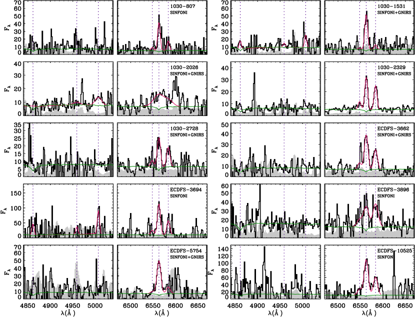
Figure 1.— One dimensional spectra in the wavelength region around H$\beta$ and [O iii] $\lambda\lambda$4959, 5007, and H$\alpha$ and [N ii] $\lambda\lambda$6548, 6583 of ten $K$-selected emission line galaxies at $2.0<z<2.7$. The wavelength is presented in rest-frame and the flux is given in $10^{-19}\,\rm ergs\,s^{-1}cm^{-2}\AA^{-1}$. The vertical dotted lines present the positions of the expected H$\beta$, [O iii] $\lambda\lambda$ 4959, 5007, [N ii] $\lambda$6548, H$\alpha$ and [N ii] $\lambda$6583 lines. The red line presents the best fit to the three emission lines. The green line is the best continuum fit to the low-resolution GNIRS spectra. Gray shaded areas present the noise spectrum. For several galaxies we combined the SINFONI with the GNIRS spectra for reasons explained in the text.

2.3. SINFONI Spectra

We observed the ten emission line galaxies with near-infrared integral-field spectrograph SINFONI during two runs, on 2005 December 10-13 (076.A-0464) and 2006 March 3-4 (076.A-0718). The weather conditions during both runs were fairly stable, with a median seeing of 0$\farcs$4 in the NIR. We use the H+K grating ($R\sim 2000$, $\lambda=14500-25000$Å) over the 8″$\times$ 8″ field of view (FOV). The FOV is sliced into 32 slitlets, and the spatial sampling corresponding to this configuration is 0$\farcs$25 $\times$ 0$\farcs$125. We observed the galaxies according to an ABA’B’ on-source dither pattern. The offset between A and B is half the FOV (4″) in the directions perpendicular to the slitlets. The offset between A and A’ is only 1″. This dither pattern enables an accurate background subtraction, as we observe empty sky on both sides of the object in each slitlet.

The raw SINFONI spectra were reduced using custom IDL scripts that perform the following steps. We start by correcting for the detector response by dividing by the lamp flats. Next, we determine the positions of the spectra on the detector for each slitlet from the “distortion frames”. These frames are constructed by moving an illuminated fiber in the direction perpendicular to the slitlet over the FOV. For every slitlet spectrum we determine the position with respect to the other spectra at each wavelength by tracing the illuminated fibre. The slitlet lengths, which are different for each slitlet, are derived from the obtained fiber traces in combination with the sky emission from the raw object frames.

Next, we make a combined bad pixel map for each individual frame, that identifies cosmic rays, hot pixels and outliers. To identify cosmic rays, we first have to remove the sky emission. An initial sky removal is performed by subtracting the average of the previous and successive frame. The remaining sky residuals are removed by subtracting the median flux at each wavelength for each slitlet spectrum, using the derived locations of the spectra on the detector, and masking the object position. Next, we identify cosmic rays on the obtained images using L.A.Cosmic (van Dokkum, 2001). We add any remaining 4$\sigma$ outliers to the map as well. This map is combined with a common bad pixel map, constructed from flat and bias frames. In what follows the combined bad pixel map will be transformed in the same way as the science images.

We return to the raw images and again we perform a simple sky-subtraction, now using the bad pixel map to reject cosmic-rays and other defects. Next, we cut and straighten all spectra, using the derived positions. For each slitlet spectrum, we straighten the skylines and perform the wavelength calibration in one step, so that the data are resampled only once. Now, we can accurately remove remaining sky at each wavelength for each slitlet spectrum, by masking the object spectrum. The previous steps yield a 3D datacube for each exposure. Finally, we combine the data cubes of the individual exposures, using the bad pixel cubes and the offsets. The final cube is divided by a response spectrum, created from the spectra of AV0 stars, matched in airmass, and reduced in a similar way as the science objects.

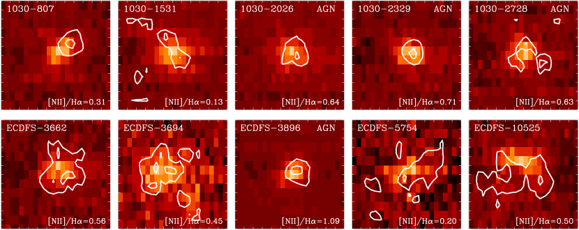
Figure 2.— 3″ by 3″ images ($\sim$25 by 25 kpc) of the continuum (color scale) and line (contours) emission. The continuum emission is derived from the median collapsed H+K SINFONI cubes, excluding wavelength regions with low atmospheric transmission or strong sky emission. The linemaps include both the H$\alpha$ and [N ii] $\lambda$6583 emission. The contours represent the 50% and 90% of the maximum line emission in the galaxy. Three of the four AGN candidates exhibit compact line and continuum emission.

2.4. Extraction of one-dimensional spectra

We extract the 1D spectra in two different ways depending on whether the H$\alpha$ and [N ii] emission lines are blended due to a strong velocity gradient. For these galaxies (ECDFS-3694 and ECDFS-10525) we remove the relative velocity shifts along the spatial direction before constructing a 1D spectrum, in order to obtain more accurate line measurements and ratios. While information on the total velocity dispersion is thereby lost, this procedure is justified for the purpose of extracting the integrated line fluxes for the analysis presented in this paper.

For both methods we start by binning the final SINFONI cubes in the spatial direction, to combine the ‘spaxels’ of 0$\farcs$125 by 0$\farcs$25 to spatial elements of 0$\farcs$25 by 0$\farcs$25. As we are mainly interested in studying the spectrum of the line-emitting gas rather than the continuum emission, we optimize the extraction of the 1D spectra in the wavelength range around H$\alpha$ and [N ii]. We make an average reconstructed image of the data cube in the wavelength region around these lines. The wavelength region within twice the velocity dispersion of the lines is included, avoiding wavelengths with strong OH lines or low atmospheric transmission. Note that the velocity dispersion is still unknown at this stage, so we have to iterate a few times to obtain the correct extraction region and the velocity dispersion. For galaxies with a velocity gradient, we take into account the relative velocity shift as well to determine which wavelength region is included

Next, we select all adjacent pixels in the reconstructed image with a flux exceeding 0.20-0.55 times the flux of the spatial element with the most signal. This threshold value is dependent on the S/N of the line emission in the reconstructed images. In case no velocity gradient is present, the 1D spectra of the selected spatial elements are combined to form the final 1D spectrum. A 1D noise spectrum is constructed from the spectra of all spatial elements that do not exceed this threshold.

For the galaxies with a velocity gradient, we fit the spectra of all selected spatial elements following the fitting procedure described in § 2.5. To avoid the residuals of skylines as being interpreted as lines, and to reduce the number of degrees of freedom, we fix the width to the velocity dispersion of the final spectrum. The allowed redshift is also constrained to a certain range, depending on the maximum velocity shift of the galaxy. Note that these latter two requirements need a few iterations. We measure H$\alpha$ and the two [N ii] lines in the spectra of all selected spatial elements, and retain the elements for which H$\alpha$ and [N ii] $\lambda$ 6583 have a total signal-to-noise (S/N) $>5$. We visually inspect the spectra of each element to check if the lines are correctly interpreted. The rest-frame 1D spectra of these selected spatial elements are averaged together to form the final 1D spectrum. We constructed a final noise spectrum by quadratically adding the rest-frame noise spectra.

Finally, we added the 1D spectra to the previously measured GNIRS spectra in cases where the S/N is low and the SINFONI data show no evidence for strong velocity gradients.

Table 3Emission line modeling results

id	$\sigma$	$W_{\rm H\alpha}$	$W_{\rm[NII]}$	$W_{\rm H\beta}$	$W_{\rm[OIII]}$	[N ii]/H$\alpha$	[O iii]/H$\beta$	[O iii]/H$\beta$
1030-807	115${}^{+21}_{-52}$	61.7${}^{+13.1}_{-8.6}$	18.7${}^{+3.1}_{-14.5}$	13.0${}^{+6.4}_{-5.9}$	-1.1${}^{+2.6}_{-2.0}$	0.33${}^{+0.05}_{-0.25}$	$<$ 0.83	$<$ 0.86
1030-1531	72${}^{+54}_{-47}$	62.8${}^{+18.8}_{-4.9}$	7.6${}^{+6.1}_{-12.2}$	9.5${}^{+1.6}_{-1.2}$	11.0${}^{+2.7}_{-3.1}$	$<$ 0.35	1.37${}^{+0.31}_{-0.37}$	$<$ 1.99
1030-2026	434${}^{+117}_{-64}$	32.9${}^{+7.2}_{-12.5}$	21.0${}^{+11.1}_{-6.4}$	2.0${}^{+3.2}_{-5.2}$	14.3${}^{+4.6}_{-1.1}$	0.64${}^{+0.61}_{-0.20}$	$>$ 1.84	$<$ 9.70
1030-2329	80${}^{+19}_{-13}$	51.1${}^{+5.3}_{-5.4}$	34.5${}^{+4.7}_{-4.1}$	7.6${}^{+2.8}_{-1.4}$	3.2${}^{+5.2}_{-2.5}$	0.71${}^{+0.08}_{-0.06}$	$<$ 2.30	$<$ 2.51
1030-2728	114${}^{+29}_{-39}$	32.4${}^{+6.9}_{-4.9}$	19.4${}^{+5.1}_{-5.3}$	3.7${}^{+2.1}_{-1.9}$	0.9${}^{+2.5}_{-1.8}$	0.63${}^{+0.17}_{-0.19}$	-	$<$ 1.77
ECDFS-3662	141${}^{+32}_{-20}$	54.6${}^{+10.7}_{-4.4}$	29.4${}^{+6.8}_{-6.8}$	2.4${}^{+5.3}_{-1.5}$	1.8${}^{+0.4}_{-3.9}$	0.56${}^{+0.09}_{-0.14}$	-	$<$ 1.06
ECDFS-3694	139${}^{+19}_{-19}$	95.8${}^{+16.5}_{-5.7}$	41.5${}^{+9.0}_{-4.5}$	28.7${}^{+17.1}_{-9.1}$	48.9${}^{+10.7}_{-3.4}$	0.45${}^{+0.05}_{-0.04}$	2.01${}^{+1.28}_{-0.67}$	$<$ 4.88
ECDFS-3896	265${}^{+10}_{-64}$	31.5${}^{+11.4}_{-2.5}$	34.1${}^{+11.4}_{-6.6}$	5.7${}^{+1.9}_{-5.0}$	2.2${}^{+1.9}_{-2.3}$	1.09${}^{+0.31}_{-0.34}$	-	$<$ 1.32
ECDFS-5754	160${}^{+17}_{-24}$	76.9${}^{+7.3}_{-7.4}$	15.4${}^{+14.3}_{-5.7}$	22.3${}^{+9.8}_{-11.7}$	5.1${}^{+7.7}_{-6.0}$	0.20${}^{+0.19}_{-0.07}$	$<$ 1.87	$<$ 2.21
ECDFS-10525	202${}^{+29}_{-0}$	116.7${}^{+13.1}_{-3.5}$	57.9${}^{+9.7}_{-1.4}$	7.8${}^{+12.7}_{-8.0}$	-5.2${}^{+5.4}_{-3.5}$	0.50${}^{+0.06}_{-0.03}$	-	$<$ 0.35
CDFS-6036	-	99${}^{+10}_{-10}$	60${}^{+6}_{-6}$	12${}^{+5}_{-5}$	99${}^{+10}_{-10}$	0.58${}^{+0.09}_{-0.08}$	8.28${}^{+5.39}_{-2.53}$	-

Note. — The errors present the best 68% confidence intervals derived using 500 Monte Carlo simulations. All upper and lower limits are 2$\sigma$. The emission lines ratios present the flux ratios.

Diagnostic diagram for spectral classification of AGNs and star-forming galaxies. The gray-scale presents the locus of $\sim$400 000 SDSS galaxies (Kauffmann et al., 2003b; Tremonti et al., 2004). The orange solid line is the empirical division between galaxies for which the line emission originates from H ii regions and AGNs for the SDSS galaxies by Kauffmann et al. (2003b). The orange dashed line presents the theoretical upper limit by Kewley et al. (2001) for star forming galaxies. Galaxies between these two dividing curves are classified as composite H ii-AGN galaxies by Kewley et al. (2006). The orange dotted line presents the division between Seyfert 2s and LINERs by Kauffmann et al. (2003b). The red filled squares present galaxies with a specific SFR (derived from modeling the continuum spectra) less than 0.05 Gyr^-1, and the blue filled circles galaxies with higher specific SFRs ($>0.05\,\rm Gyr^{-1}$). Furthermore, the green squares indicate galaxies with compact line emission. The galaxies with black circles are identified as AGN candidates, based on their [N ii]/H$\alpha$ ratios, spatial extent of the line emission, and ancillary data. Further details are in the text. All upper limits are 2$\sigma$ and the error-bars are all 1$\sigma$. For 1030-2026 we have both a 2$\sigma$ upper and lower limit.

2.5. Line measurements

We obtain emission line ratios, velocity dispersions and equivalent widths of the emission lines by modelling the extracted 1D spectra. The $H$ and $K$ spectral bands were fit separately. The $H$ band contains the lines H$\beta$ and [O iii] $\lambda\lambda$4959, 5007. The $K$ band covers H$\alpha$ and [N ii] $\lambda\lambda$6548, 6583. We fit Gaussian models to each set of lines simultaneously, assuming a similar width for all three lines and one redshift. We note that the different emission lines may not have similar line width as they can originate from different physical processes. However, as we will use the emission line measurements to identify the main contributor to the line emission, we assume that all lines originate from the same emission line region. Furthermore, the [N ii] and H$\alpha$ lines have similar widths for the galaxies for which we could measure the lines separately.

We adopt the ratios of transition probablity between the two [N ii] lines and the two [O iii] lines of 0.34 and 0.33 respectively. Thus, for each fit there are four free parameters: redshift, line width, and the fluxes of the two emission lines. The line widths were fixed to the best-fit value obtained from the set of emission lines (either H$\beta$ and [O iii] $\lambda\lambda$4959, 500 or H$\alpha$ and [N ii] $\lambda\lambda$6548, 6583) with the highest S/N. For the continuum we use the best fit to the GNIRS low-resolution continuum spectra, corrected for velocity broadening, assuming that the stellar dispersion is similar to the gas dispersion. Thus the continuum directly includes the Balmer absorption.

The 1D spectra are fitted by minimizing the absolute residuals from the fit weighted by the noise spectrum. This fitting method is preferred over $\chi^{2}$ fitting, as it minimizes the influence of sky lines and strong noise peaks. Errors on the flux measurements were determined by fitting 500 simulated spectra, that were constructed from the original spectrum and the photon noise. In these simulations we also varied the continuum according to the probability distribution that followed from modeling the GNIRS spectra. In cases where we fix the width, as derived from a brighter emission line in the same spectrum, we also vary the assumed width in the simulations according to the corresponding probability distribution.

For all galaxies except 1030-2026, we start by fitting H$\alpha$ and the [N ii] lines. We use the obtained redshift, line width and its probability distribution to fit H$\beta$ and the [O iii] lines. For 1030-2026 H$\alpha$ is strongly blended with the [N ii] lines, even in the higher resolution SINFONI spectra. As this galaxy has a clear [O iii] $\lambda$5007 detection in both SINFONI and GNIRS spectra, we swap the order. Thus for this galaxy we first derive the redshift, the line width, and its probability distribution from modeling [O iii] and H$\beta$. Using the derived redshift, line width and its probability distribution, we can now measure H$\alpha$ and the [N ii] lines.

Figure 1 shows the 1D spectra and best-fit model for all detected emission lines. The final 1D spectra include the SINFONI data, or a combination of both SINFONI and GNIRS. As the SINFONI extraction method is optimized for the line emitting gas, and the GNIRS for the continuum, the final 1D spectra may not be representative for the whole galaxy. Nevertheless, a comparison between GNIRS and SINFONI for the galaxies which could be measured separately, show that the $W_{\rm H\alpha}$’s are in good agreement: ECDFS-10525: $W_{\rm H\alpha,GNIRS}=116^{+12}_{-11}$Å and $W_{\rm H\alpha,SINFONI}=117^{+13}_{-4}$Å; 1030-807: $W_{\rm H\alpha,GNIRS}=56^{+3}_{-13}$Å and $W_{\rm H\alpha,SINFONI}=62^{+13}_{-9}$Å; ECDFS-3694: $W_{\rm H\alpha,GNIRS}=125^{+15}_{-9}$Å and $W_{\rm H\alpha,SINFONI}=96^{+17}_{-6}$Å.

The best-fit equivalent widths, line widths and emission line ratios are listed in Table 3. The values for the emission line ratios are given when both lines have a $>2\sigma$ detection. In case only one of the two lines has a $>2\sigma$ detection we give a $2\sigma$ upper or lower limit. As can be seen in Figure 1 H$\alpha$ is detected for all galaxies, and [N ii] $\lambda$6583 can be measured for nine of ten galaxies. Thus, we can determine the value for [N ii]/H$\alpha$ for these nine galaxies. For 1030-1531, which has no [N ii] detection we give a 2$\sigma$ upper limit. For only two galaxies both H$\beta$ and [O iii] $\lambda$5007 are detected at $>2\sigma$. For these galaxies the ratio [O iii]/H$\beta$ can be measured directly. For four objects we obtained lower or upper limits from the fitting procedure, as one of the two lines (H$\beta$ or $\lambda$5007) had a 2$\sigma$ detection. For example, for galaxy 1030-807 the H$\beta$ line is detected at 3 sigma and [O iii] $\lambda$5007 has an upper limit. Thus, we can derive a 2$\sigma$ upper limit on [O iii]/H$\beta$, from the 97.5% cut of the best-fit [O iii]/H$\beta$ values of the 500 simulations. For the remaining four galaxies the modeling results yielded no limit on [O iii]/H$\beta$, as neither of the two lines was detected.

For all galaxies we apply a second method to constrain [O iii] $\lambda$5007/H$\beta$, based on the intrinsic ratio of H$\alpha$/H$\beta$ ($=2.76$). We determine a 2$\sigma$ lower limit on H$\beta$ from the 2$\sigma$ lower limit on H$\alpha$. Furthermore, we attenuate H$\beta$ using the 2$\sigma$ upper limit on the best-fit modeled $A_{V}$ and assuming extra extinction towards H ii regions (factor of 0.44 in $A_{V}$, Calzetti, 1997; Calzetti et al., 2000). We combine the attenuated 2$\sigma$ lower limit on H$\beta$ with the modeled 2$\sigma$ upper limit on [O iii] $\lambda$5007 to derive the 2$\sigma$ upper limit on [O iii]/H$\beta$. The limits are listed for each galaxy in the last column of Table 3.

The H$\alpha$ line of 1030-2026 is not well fitted in Figure 1. This is not caused by a wrong redshift measurement, as we know the redshift of this galaxy very accurately from the [O iii] $\lambda$5007 line. There seems to be a second peak at a rest-frame wavelength of 6600 Å. Although this “line” falls on top of a strong OH line, the emission feature looks real in the 3D cube. It could well be H$\alpha$ emission from a companion galaxy or a star forming region located in the outer parts of the galaxy.

2.6. Line maps

For each galaxy we make reconstructed images of the continuum and line emission separately. The continuum images includes all observed H+K emission, excluding wavelengths with low atmospheric transmission or strong sky emission. The linemaps include both the H$\alpha$ and the [N ii] $\lambda$6583 emission. The S/N is not high enough to make linemaps of these two components separately. We included the line emission within two times the velocity dispersion of the emission lines, accounting for a velocity gradient if present. The continuum emission is removed using the flux measurements in the wavelength range surrounding the lines. Finally, we convolve the line map by a boxcar of 3 pixels (0$\farcs$375), to smooth out the noise.

Maps of the continuum and line emission are presented in Figure 2. The spatial sampling of the reconstructed images is 0$\farcs$125 by 0$\farcs$25, unlike the reconstructed images used to extract the spectra, which are binned to 0$\farcs$25 by 0$\farcs$25. The area over which the 1D spectra are extracted is about similar to what is included by the outer contours.

3. ORIGIN OF THE LINE EMISSION

A key goal of this paper is to elucidate the origin of the H$\alpha$ emission detected in slightly over half of the massive galaxies in our sample. In the local universe, H$\alpha$ emission is usually an indicator of star formation, and the luminosity of H$\alpha$ directly correlates with the instantaneous star formation rate (Kennicutt, 1998). However, other processes can also ionize Hydrogen, in particular hard radiation from a central active nucleus. In this section we use different indicators for star formation and AGN activity to determine the nature of the population of emission-line galaxies.

3.1. Emission line ratios

Local star-forming galaxies in the SDSS follow well-defined tracks in diagnostic diagrams featuring various emission line ratios (e.g. Baldwin et al., 1981; Veilleux & Osterbrock, 1987). For our sample, the appropriate diagram is [O iii] $\lambda$5007/H$\beta$ versus [N ii] $\lambda$6583/H$\alpha$  as these lines are relatively strong and are covered in both our GNIRS and our SINFONI spectra. This diagram is shown in Figure 3. Galaxies for which lines originate from photo-ionization by young stars in H ii regions fall on the well-defined sequence. Local galaxies outside this metallicity driven sequence are dominated by other ionization sources, typically photo-ionization by a hard spectrum such as produced by an AGN.

Kauffmann et al. (2003b) empirically separates the AGNs from the H ii sequence by the solid line in Figure 2.4. The extreme starburst classification line derived by Kewley et al. (2001) is presented by the dashed line. The galaxies between these two dividing lines are classified as composite H ii-AGN galaxies by Kewley et al. (2006). However, both Erb et al. (2006a) and Shapley et al. (2005) suggest that the H ii driven sequence is offset to the right at high redshift. Thus, we have to be careful when applying the classification scheme as derived for local galaxies to our high-redshift sample, as the behavior of the ionization ratios at high redshift is not well understood. The galaxies outside the H ii sequence are generally divided into LINERs and Seyfert 2s. The dotted line in Figure 2.4 is the dividing line by Kauffmann et al. (2003b).

Our eleven emission line galaxies are indicated by the red filled squares (specific SFR $<0.05$ Gyr^-1) and blue filled circles (specific SFR $>0.05$ Gyr^-1) in Figure 2.4. Remarkably, only four objects fall in the region of galaxies with pure star formation as defined by Kewley et al. (2006), while the other seven galaxies are classified as AGN or composite H ii-AGN. Three of these galaxies fall in the Seyfert 2 regime, three galaxies may be LINERs or Seyfert 2s, and one is classified as a LINER.

While Seyfert 2s are generally accepted as AGNs, the power source of LINERs is still debated. Although photo-ionization by an AGN is often the most straightforward explanation, LINER emission has also been observed in extra-nuclear regions associated with large-scale outflows and related shocks (Dopita & Sutherland, 1995; Lípari et al., 2004). Shock-producing winds can be driven by AGNs (e.g., Cecil et al., 2000; Nesvadba et al., 2006), but also by strong starbursts (e.g., Lípari et al., 2004).

The measured $W_{\rm H\alpha}$ vs. the expected $W_{\rm H\alpha}$ derived from the spectral continuum shape (see Figure 3) and the Kennicutt (1998) relation between SFR and H$\alpha$ luminosity. In case H ii regions are the only contributors to the line emission, a galaxy falls on the expected 1-to-1 relation (dotted line). Additional extinction towards star forming regions moves a galaxy downwards of the relation. Objects that fall above the dotted line most likely have another ionization source contributing to the line emission as well. The symbols are similar as in Figure 2.4.

3.2. Other diagnostics of AGN activity

Given the ambiguity in the interpretation of LINER spectra it is necessary to examine other indicators of star formation and AGN activity, to determine for which of the seven galaxies with non H ii region-like ratios an AGN is the most likely explanation (either directly through photo-ionization or through shocks produced by an AGN-driven outflow). We first consider which are the most important additional diagnostics at our disposal:

X-ray emission: As is well known AGNs can be efficiently identified by their X-ray emission, which is thought to be due to up-scattered UV photons from the accretion disk. AGN-induced X-ray emission can be distinguished from that induced by star formation by the hardness ratio and (particularly) the luminosity. For the galaxies in SDSS1030 we use XMM data with a depth of 100 ks (Uchiyama et al. 2006, in preparation). Three of the ECDFS galaxies (ECDFS-3662, ECDFS-3694 and CDFS-6036) are in the CDFS proper (Giacconi et al., 2002), for which very deep 1 Ms Chandra data are available. The other CDFS galaxies (ECDFS-3896, ECDFS-5754 and ECDFS-10525) are in the “Extended” CDFS, for which we use 250 ks Chandra data (Virani et al., 2006). Interestingly, only one out of seven galaxies is detected. Limits are given in Table 1. These limits indicate that the AGNs, if present, are either highly obscured or accrete at sub-Eddington rates.

Compactness: The spatial distribution of the line emission can provide information on its origin, as narrow line regions of AGNs are generally compact. However, extended line emission does not rule out the presence of an AGN for galaxies with active star formation, as star forming regions contribute to the line emission. Furthermore, AGNs can produce outflows, which may result in extended line emission. As can be seen in Fig. 2, in several galaxies the line emission is very compact whereas in others it is extended.

H$\alpha$ equivalent width: As we have estimates for the SFR in these galaxies from the stellar continuum fitting, we can compare the observed strength of H$\alpha$ to that predicted from the best-fit synthetic spectrum. An excess of H$\alpha$ emission could indicate another ionization source than star formation, such as AGN activity. We compute the predicted H$\alpha$ line luminosity using the SFR from the best-fit model to the observed continuum emission (which includes $A_{V}$ as a free parameter) and the Kennicutt (1998) relation. We then divide this estimate by the continuum luminosity density around the wavelength of H$\alpha$ as determined from the best-fit synthetic spectrum and corrected for the best-fit extinction

In Figure 3.1 we compare the measured and expected $W_{\rm H\alpha}$. The relation between the two is dependent on the dust geometry, such that extra extinction towards H ii regions would move a galaxy below the 1-to-1 relation (which is indicated by the dotted line). As it is unlikely that the attanuation in star forming sites is less than the continuum attenuation (see Cid Fernandes et al., 2005), a galaxy is not expected to lie above the dotted 1-to-1 relation. However, in case of another ionization source such as AGN activity, the measured $W_{\rm H\alpha}$ would be higher than the expected. We indeed find that several galaxies fall above the expected relation, which implies that an ionization source other than star formation may be contributing to line emission as well.

Star formation activity: If a galaxy has a high SFR the current starburst might produce an outflow which results in AGN-like emission line ratios. Although this outflow is hard to confirm, the absence of a starburst immediately rules out this scenario, and infers that ionization ratios are indeed due to AGN activity. To indicate which galaxies have an engine for such an outflow, we divided the sample in galaxies with high (blue filled circles) and low SFRs (red filed squares) in Figure 3.

Next, we assess for each of the seven candidates whether the line emission is most likely dominated by an AGN or some other process, using these criteria and others particular to individual objects. We stress that in none of the cases it is completely clear-cut: even in the local universe, with the availability of vastly superior data to ours, it is often impossible to cleanly identify the relative contributions of AGNs and star formation to the line emission (e.g., Filho et al., 2004; Kewley et al., 2006).

1030-2026: This galaxy has Seyfert 2 emission line ratios, compact line emission, and a low SFR (as implied by the continuum modeling). Thus, a starburst driven wind is very unlikely for this galaxy. Furthermore, Figure 3.1 shows that ongoing star formation, as derived from the stellar continuum, cannot account for the observed H$\alpha$ emission. Finally, the velocity dispersion of $\sim$450 km s^-1 of [O iii] $\lambda$5007 may be indicative of an AGN. We classify this galaxy as an AGN.

1030-2329: The emission line ratios of this galaxy are indicative of an AGN, or a composite H ii-AGN galaxy. The excess of H$\alpha$ emission in Figure 3.1 supports the presence of another ionization source. Furthermore, for this galaxy a starburst driven wind is very unlikely, due to the combination of a low un-obscured SFR (as implied by the continuum) and compact line emission. We include this galaxy in our AGN selection.

1030-2728: This galaxy has similar supporting diagnostics as 1030-2329, but the line emission is not compact. However, the spectrum shows hints that the [N ii] emission peaks in the central emission blob in Figure 2, while the lower-right emission peak is dominated by H$\alpha$ emission. Unfortunately, the S/N of the individual line maps is not high enough to draw firm conclusions. As all other diagnostics indicate an AGN as the dominating ionization source, we add this galaxy to our AGN selection.

ECDFS-3662: This galaxy probably falls in the composite H ii-AGN region of Figure 2.4. Unfortunately, we cannot discriminate between shock-ionization by a starburst driven outflow and an AGN, as this galaxy has a high SFR and extended line emission. Other diagnostics do not provide evidence for an AGN: the object has no X-ray counterpart (in the 1 Ms data), and is not identified as an AGN (nor ULIRG) by Alonso-Herrero et al. (2006) using the infrared continuum shape. Furthermore, the observed H$\alpha$ emission is consistent with star formation. Although we cannot rule out the presence of an AGN, we will not include this galaxy in our AGN sample.

ECDFS-3694: This galaxy is classified as a composite H ii-AGN galaxy in Figure 2.4. It has a high SFR, extended line emission, and shows a large velocity gradient of $\sim$1400 km s^-1. This galaxy falls in the field examined by Alonso-Herrero et al. (2006), and is not classified as a ULIRG or AGN according to its mid-infrared SED shape. It is undetected in the 1 Ms X-ray imaging. A starburst driven outflow seems the most plausible scenario for this galaxy, although an AGN cannot be ruled out. Thus, this galaxy will not be part of our AGN candidate sample.

ECDFS-3896: The emission line ratios for this galaxy are indicative of an AGN or a composite H ii-AGN galaxy. This galaxy has a high SFR derived from the stellar continuum, which is consistent with the observed H$\alpha$ emission. Nevertheless, a starburst driven wind is somewhat unlikely, as the line emission shows a very compact structure and the galaxy shows no velocity gradient. Furthermore, as will be discussed in the next section, the UV-emission which boosts the SFR in the model fits, may well be due to continuum emission by the AGN. Optical spectroscopy is needed to clarify this situation. As an AGN seems the most plausible cause for the emission line ratios, we include this galaxy in our AGN sample.

CDFS-6036: This galaxy seems the most convincing Seyfert 2 in Figure 2.4. Nevertheless, van Dokkum et al. (2005), who studied this object in detail, suggest that the ratios are caused by shock ionization due to a starburst-driven wind. The main evidence is the extension of the high [N ii]/H$\alpha$ ratios to the outer parts of the galaxy and the presence of a strong starburst to drive the outflow. Furthermore, the galaxy shows a strong velocity field, and both the H$\alpha$ line emission and the X-ray detection in the soft band (see Table 1) are consistent with the SFR as derived from the stellar continuum (see also Figure 3.1). The rest-frame UV spectrum of this galaxy does not show any AGN features either (Daddi et al., 2004a). The galaxy has a power-law SED ($\alpha=-1.2$), indicative of an ULIRG or AGN (Alonso-Herrero et al., 2006). As the available diagnostics are compatible with a starburst- driven wind, we conservatively do not include this galaxy in the AGN candidate sample. We note that including this object in the AGN sample would not change our conclusions.

3.3. Summary and AGN Fraction

We find that of the eleven emission line galaxies only four have emission line ratios consistent with the SDSS star forming sequence (Kauffmann et al., 2003b). The immediate implication is that other processes than “normal” star formation in H ii regions play a major role in massive galaxies at $z\sim 2.5$. Determining the nature of these processes is difficult, as many different physical mechanisms can produce very similar line diagnostics. Using a variety of indicators we argue that for four of the galaxies the most likely source of the H$\alpha$ emission is an AGN. These galaxies are indicated by large solid circles in Figures 3 and 4, and are labeled “AGN” in Figure 2 as well. They are all narrow line AGNs, as the velocity dispersions of the emission lines are less than 2000 km s^-1 (Table 3).

According to this classification, the AGN fraction among our total sample of $K$-selected galaxies at $2.0<z<2.7$ is 20% (4/20). Due to the various caveats in the AGN classification this fraction may be underestimated. First, AGNs are easier to identify in quiescent systems, than in actively star-forming galaxies, due to the strong contamination of line emission by H ii regions. This not only complicates the emission line diagnostics, but also weakens the argument of the excess of H$\alpha$ emission compared to the stellar continua, as this excess is easier to detect in galaxies with low SFRs. Optical spectroscopy may help to uncover AGNs in star-forming galaxies, by identifying rest-frame UV high-ionization emission lines such as C IV and He II. But also the MIR continuum shape and spectral features (e.g., Stern et al., 2006; Weedman et al., 2006) or very deep SINFONI spectra to reveal the spatial distribution of [N ii]/H$\alpha$ (Genzel et al., 2006; Förster Schreiber et al., 2006b; Nesvadba et al., 2006) can be used to identify AGNs in these galaxies. Furthermore, AGNs may have been missed if they are strongly obscured (mid-infrared data is available for only a few galaxies), or are just too faint to be detected. On the other hand, we cannot rule out shocks produced by a starburst driven wind as the origin of the line emission in at least one of the four candidates.

Papovich et al. (2006) find an AGN fraction of 25% among a sample of distant red galaxies (DRGs, Franx et al., 2003) at $1.5<z<3.0$, using X-ray imaging and the shape of the mid-infrared continuum. This result is consistent with our fraction, given the fact that DRGs make up to 70% of the massive galaxy population at $2<z<3$ (van Dokkum et al., 2006). Our result is also consistent with the result of van Dokkum (2004), who find at least two AGNs among a sample of six emission line DRGs. Although Rubin et al. (2005) find an AGN fraction of only 5% among the 40 DRGs in the FIRES MS 1054 field (Förster Schreiber et al., 2006a), their criterion of $L_{X}>1.2\times 10^{43}$ ergs s^-1 would almost certainly not pick up any of the four AGNs in our study.

Our fraction of AGNs among $K$-selected galaxies is significantly higher than among UV-selected galaxies. Erb et al. (2006b) identify AGNs in 5 out of 114 UV-selected galaxies, based on the presence of broad and/or high ionization emission lines in the rest-frame UV spectra, broad H$\alpha$ lines, or very high [N ii]/H$\alpha$ ratios (see Erb et al., 2006b). This fraction is similar to the 5% found by Reddy et al. (2005) among the full spectroscopic sample of UV-selected galaxies using direct detections in the 2-Ms Chandra Deep Field North images, and 3% found by Steidel et al. (2002) among a sample of 1000 LBGs at $z\sim 3$, using rest-frame UV spectroscopy. The comparison is complicated as all studies use different selection criteria. However, this cannot explain the substantial difference in AGN fraction between the UV and $K$-selected galaxy samples. We will return to this issue in § 4.2.

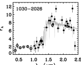
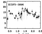
Figure 3.— Binned “low resolution” spectra (filled squares) and optical-to-NIR photometry (open circles) of the 4 AGN host galaxies. The best-fit stellar population models are drawn in gray. The detection of strong Balmer and/or 4000 Å breaks in three of the four galaxies implies that the continuum emission in these galaxies is dominated by stellar light. The SED of ECDFS-3896 indicates active star formation in this galaxy, while the other three galaxies are best fitted by evolved stellar populations.

Stacked GNIRS spectra and composite broadband SEDs of the three different classes of galaxies in our sample: the nine quiescent galaxies without detected emission lines, the four AGN candidates, and the remaining seven emission line galaxies. The individual GNIRS spectra were normalized in the wavelength interval between 4000 Å and 6000 Å, and the individual broadband SEDs were set to unity at a wavelength of 5000 Å. The dotted vertical lines present from left to right the location of [O ii] $\lambda$3727, Ca(H), Ca(K), H$\delta$, H$\gamma$, H$\beta$, [O iii] $\lambda$4959, [O iii] $\lambda$5007, H$\alpha$  [N ii] $\lambda$6583. The gray lines in the lower panels show the average of the individual best-fit stellar population models to the spectra and broadband photometry for each class.

4. IMPLICATIONS

In the previous section we identified four AGN candidates among the eleven emission line galaxies in our $K$-selected sample. In this section we discuss the nature of the host galaxies of these AGNs, and what this implies for our understanding of the role of AGNs in the star formation history of galaxies.

4.1. Stellar populations of AGN host galaxies

The low resolution GNIRS spectra and broadband SEDs for all four AGN candidates are presented in Figure 3. The strong optical breaks for three out of four galaxies imply that the continuum emission in these galaxies is dominated by stellar light. This is less clear for ECDFS-3896, as the spectrum of this galaxy shows only a weak break. The best-fit stellar population models to the spectrum and the optical photometry, when assuming that the continuum emission originates from stars only, are also shown in Figure 3. The corresponding population properties are listed in Table 2. The spectral continuum of three galaxies (1030-2026, 1030-2329 and 1030-2728) are best fit by evolved stellar population models with low SFRs, while ECDFS-3896 is actively forming stars. However, as the continuum emission from the AGN might contribute significantly, the derived stellar mass and population properties for this galaxy are quite uncertain.

The median absolute and specific SFRs (SFR per unit mass) of the AGN host galaxies are 9 $M_{\odot}\,\rm yr^{-1}$ and 0.04 Gyr^-1 respectively. To examine how the stellar populations of the AGN hosts compare to those in other galaxies in this redshift range, we divide the total $K$-selected sample into three classes: the quiescent galaxies without detected emission lines (Kriek et al., 2006b), the AGNs, and the remaining emission line galaxies. In Figure 3.3 we show the stacked spectra and composite broadband SEDs of these three classes. The stacked spectra are constructed from the individual GNIRS spectra, normalized over the continua between a rest-frame wavelength of 4000 and 6000 Å. We applied a noise weighted stacking method to avoid the influence of sky lines and wavelength regions with bad atmospheric transmission. The broadband SEDs are normalized at a rest-frame wavelength of 5000 Å. We also show the average of the individual best-fit stellar population models to the spectra and broadband SEDs in the lower panels. Note that for the quiescent galaxies the redshifts are derived from the continuum shape. As we have less precise redshift measurements for these galaxies, spectral features will be smoothed out.

Figure 3.3 illustrates that the average spectrum and broadband SED of the AGN hosts is intermediate between the star-forming and quiescent galaxies, although more similar to the latter. However, this result may be biased, as AGNs are easier to identify in galaxies with low SFRs (see § 3.3). Thus, we cannot draw firm conclusions on the stellar populations of the full class of AGN hosts. Nevertheless, the low SFRs in three of the AGN host galaxies may suggest that the AGN activity is related to the suppression of the star formation.

$R-K$ and the specific SFR (as derived from the stellar continua) vs. the stellar mass for both the UV-selected galaxies by Erb et al. (2006a, b, c) and our spectroscopic $K$-selected sample at $2.0<z<2.7$. The masses for the UV and $K$-selected samples are derived from modeling the broadband photometry and the stellar continua respectively, assuming a Salpeter (1955) IMF. The galaxies in which AGNs are identified are indicated in black. The shaded gray areas in both diagrams are empty probably because of incompleteness effects. We can roughly remove the bias towards AGN with more massive black holes, by normalizing the star-formation rate by the stellar mass, assuming that it scales with the black hole mass. Considering a line of constant specific SFR the line emission originating from accretion onto the black hole should be equally easy to detect as the line emission from star formation. Thus, AGNs with the same normalized accretion rate should have been detected in the area between the dotted lines and to the right of the shaded region. This figure illustrates that black hole accretion is more effective at the high-mass end at $z\sim 2.3$.

4.2. Stellar masses of AGN host galaxies

In order to asses why the AGN fraction among the UV-selected galaxies by Erb et al. (2006a) is much lower than among our $K$-selected sample, we plot the $R-K$ and the specific SFR versus the stellar mass for both samples in Figure 4.1, indicating the AGNs in black. Remarkably, the stellar masses of the AGN host galaxies in both samples are similar: 2.8$\times$10${}^{11}M_{\odot}$ and 3.0$\times$10${}^{11}M_{\odot}$ for the UV- and $K$-selected galaxies respectively (for a Salpeter IMF). As the galaxies in the $K$-selected sample all have similar stellar masses, an under- or overestimation of the AGN fraction will not change this result significantly. This preference for massive galaxies may be the main reason why AGNs are more common among $K$-selected than among UV-selected galaxies.

The apparent mass dependence of AGN host galaxies is affected by selection effects. The difference in $R-K$ color and specific SFRs among the $K$-selected and UV-selected AGN host galaxies is most likely caused by the different sample selections, as three of our AGN hosts are too faint in the rest-frame UV to be picked up by the BM/BX technique (Steidel et al., 2004). Three out of seven AGNs in Figure 4.1a have $R-K>5.2$. Due to the limitations of both surveys, we have no information about galaxies with $R-K>5.2$ and stellar masses below 10${}^{11}M_{\odot}$, and it could be that AGNs reside in these galaxies as well. However, even if we ignore all galaxies with $R-K>5.2$ a strong mass-dependency is apparent in Figure 4.1a.

One can argue that this stellar mass dependency of AGN host galaxies simply reflects the decrease of black hole mass ($M_{\rm BH}$) when going to lower mass galaxies, which would make the AGNs more difficult to detect relative to the contribution from star formation. We cannot address this bias fully with currently available data, but we can roughly estimate the effect by normalizing the star formation rate by the stellar mass (Fig. 4.1b). Considering a line of constant specific SFR, and assuming that the black hole mass scales with the stellar mass of a galaxy (e.g., Desroches et al., 2006), the line emission originating from accretion onto the black hole should be equally easy to detect as the line emission from star formation. However, at a specific SFR between 0.1 Gyr^-1 and 1.6 Gyr^-1 we only find AGNs in very massive galaxies. This implies that the black hole accretion at high redshift is most effective at higher masses.

This ignores the effect of variations in extinction, which are known to occur in these samples. In case star formation is more extincted at the high mass end, AGN emission might be easier to detect in these galaxies. We also note that the samples are incomplete in the shaded areas indicated in Figure 4.1. Furthermore, the stellar masses and specific SFR derived for ECDFS-3896 and the UV-selected galaxies might be affected by continuum emission from the AGN.

4.3. Downsizing of AGN host galaxies

Deep X-ray studies suggest that the AGN population exhibits cosmic downsizing, as the space density of AGNs with low X-ray luminosities peaks at lower redshift than that of AGNs with high X-ray luminosities (Steffen et al., 2003; Ueda et al., 2003; Hasinger et al., 2005). Using the SDSS galaxies Heckman et al. (2004) conclude that this behavior is driven by a decrease in the characteristic mass scale of actively accreting black holes. As the total stellar mass and black hole mass are found to correlate (e.g., Desroches et al., 2006), the stellar mass of AGN hosts may be expected to decrease as well, when going to lower redshift.

To explore the behavior of the stellar mass of AGN hosts with redshift, we compare the AGN fractions of galaxies with similar normalized accretion rates at high and low redshift per stellar mass bin in Figure 4.3. The high-redshift galaxies are indicated by the symbols with error-bars. For the UV-selected galaxies we only use the mass-range to the right of the dashed line indicated in Figure 4.1b, as we cannot ensure the detection of AGNs at lower stellar masses. The fraction peaks at $M\sim 2.9\times 10^{11}M_{\odot}$, but as explained in the previous subsections, this may be due to incompleteness effects.

In order to compare our sample with low-redshift AGNs with a similar normalized accretion rate we impose a threshold for $L_{\rm[NII]}/M_{*}$, assuming that the black hole mass scales with the stellar mass. For the low-redshift galaxies we use the same SDSS galaxy sample and AGN classification by Kauffmann et al. (2003b), as plotted in Figure 2.4. We required a $>3\sigma$ detection for both H$\alpha$ and [N ii]. In case [O iii]/H$\beta$ could not be determined, we selected AGNs by log([N ii]/H$\alpha$)$>-0.2$. We set the normalized accretion threshold to the minimum luminosity of all detected [N ii] lines in our sample – as AGNs with these luminosities would have been detected – divided by the median stellar mass of the AGN hosts in our sample.

At low redshift the accretion rate is often parametrized by the luminosity of [O iii] (e.g., Heckman et al., 2005). As [O iii] is not detected for most of our galaxies, we use the luminosity of [N ii] instead. For AGNs in the local universe there is a broad positive correlation between the two (see Figure 3), although this correlation is different for LINERs and Seyfert 2s. Nevertheless, [N ii] is acceptable for our purpose, as we only use the line luminosity to determine a normalized accretion threshold to compare similar samples at low and high redshift, which include both LINERs and Seyfert 2s.

Figure 4.3 shows that SDSS AGN hosts with a similar normalized accretion rate as our high-redshift AGNs reside in lower mass galaxies ($\sim 4\times 10^{10}M_{\odot}$). This finding provides direct observational support that cosmic downsizing of AGNs is related to the decrease of the characteristic stellar mass of their host galaxies (see also Heckman et al., 2004). This conclusions is fairly robust, and is not strongly dependent on the threshold value $L_{\rm[NII]}/M_{*}$, or whether we would use a threshold based on the luminosity of [O iii] instead: a factor 2 or 3 difference barely changes the stellar mass at which the AGN fraction peaks at low redshift. The main concern for using the [O iii] or [N ii] emission lines as indicators for the accretion rate is the contamination by star formation. However, in case [N ii] at $z\sim 2.3$ is more contaminated by star formation than at $z\sim 0$, our normalized “threshold accretion rate” would be overestimated, and we would select less galaxies at low redshift, and find a slightly lower typical stellar mass.

Figure 4.3 also shows the total AGN fraction (i.e., including fainter AGNs) among the SDSS galaxies versus stellar mass. This distribution, which is dominated by faint AGNs, peaks at higher stellar masses. This implies that at similar stellar masses of the host galaxies, AGNs in massive galaxies at low redshift are less powerful than those at high redshift. These low-redshift AGNs may be the low luminosity descendants of the AGNs observed in our $K$-selected galaxies.

Both these conclusions would be qualitatively similar if our AGN fraction would be slightly over- or underestimated, as the galaxies in our sample span only a small range in stellar mass.

Fraction of actively accreting AGN among galaxies in different mass bins at different redshifts. The red diamonds present the AGN fraction for the 20 $K$-selected galaxies at $2.0<z<2.7$. The purple squares present the AGN fraction among the UV-selected galaxies at $z\sim 2.2$ by Erb et al. (2006a). The rapid fall off of both histograms may be due to selection effects. The blue histogram is the fraction of AGNs in the SDSS sample (Kauffmann et al., 2003a) with similar normalized accretion rates as the AGNs in our $K$-selected sample. The green histogram are all AGNs in the SDSS, as defined in the text. All stellar masses are derived from stellar population modeling, and converted to a Salpeter (1955) IMF. This diagram illustrates that actively accreting AGNs reside in more massive galaxies at higher redshift.

Rest-frame $u-g$ color and $D_{\rm n}(4000)$ vs. stellar mass for the $K$-selected $2.0<z<2.7$ galaxy sample. Both properties ($u-g$ and $D_{\rm n}(4000)$) are derived from the best fits to the rest-frame optical continuum spectra in combination with the rest-frame UV broad-band photometry. The errors are derived from the 68% best-fits of 200 Monte Carlo simulations. The gray scale presents the low-redshift catalogue of galaxies extracted from the SDSS by Blanton et al. (2005). The photometric masses (Kauffmann et al., 2003a) are corrected for the difference in assumed IMF with the $K$-selected sample. The actively accreting AGNs within the SDSS sample, as defined in § 4.3 are represented by the orange contours. The evolution of a stellar population for two different SFHs with different decaying times ($\tau$) are drawn, assuming a formation redshift of 2.8. The ages are indicated in Gyr. These diagrams may suggest that both at low and high redshift the AGN activity peaks during the post-starburst phase, when a galaxy is transforming from a star-forming into a quiescent galaxy.

4.4. AGNs and the suppression of star formation

The decrease of the stellar mass of actively star-forming galaxies with redshift (Cowie et al., 1996; Juneau et al., 2005) may imply that the stellar mass at which the star formation is suppressed also decreases over cosmic time. Bundy et al. (2006) introduce a critical “quenching mass”, which declines significantly between a redshift of 1.4 and 0.5, and drops even further at low redshift, as the galaxy bi-modality in the SDSS breaks down at a stellar mass of $3\,\times\,10^{10}M_{\odot}$ (Kauffmann et al., 2003a). Also, theoretical studies derive critical quenching masses, above which cooling and star formation are shut down abruptly (e.g., Cattaneo et al., 2006).

Due to incompleteness of our sample, especially at lower stellar masses, we cannot derive a critical quenching mass for the observed redshift range. Nevertheless, Figure 4.3 illustrates that in contrast with low redshift, the high-mass end at $z\sim 2.3$ consists of both star-forming galaxies and red, quiescent systems. Moreover, the red, passive systems may dominate the galaxy population beyond $2.5\,\times\,10^{11}M_{\odot}$ (see Figure 4.3). This may imply that the transition from star-forming to quiescent galaxies at $z\sim 2.3$ occurs at the observed mass range.

Remarkably, at both low and high redshift, the fraction of actively accreting AGNs may peak at a similar stellar mass range at which the suppression of the star formation seems to occur (see also Heckman et al., 2004). This may imply that the critical quenching mass tracks the evolution of the typical stellar or black hole mass at which active accretion takes place. This is illustrated in Figure 4.3, which shows the rest-frame $u-g$ color and $D_{n}(4000)$ versus the stellar mass for both our $K$-selected sample and the 28 000 low-redshift SDSS galaxies with estimated co-moving distances in the range $10<d<150\,\rm Mpc~{}h^{-1}$ by Blanton et al. (2005) (this is a sub-sample of the SDSS galaxies presented in Figures 2.4 and 4.3). $D_{n}(4000)$ measures the ratio of the average flux density $F_{\nu}$ in the bands 4000-4100 Å and 3850-3950 Å around the break (Balogh et al., 1999). The actively accreting low-redshift AGNs are identified by the orange contours.

The AGN hosts at low and high redshift seem to have similar $D_{n}(4000)$ and rest-frame $u-g$ colors. However, as explained in Section 3.3, AGNs in star forming galaxies may have been missed, and this would lower the typical $D_{n}(4000)$ and rest-frame $u-g$ colors of AGN host galaxies. We note however, that the AGN classification in the SDSS probably suffers from a similar effect. Sánchez et al. (2004) and Nandra et al. (2006) find a similar location for AGNs in color space – in the “green valley” between the red sequence and blue cloud – for optically and X-ray selected AGNs at $0.5<z<1.1$ and $0.6<z<1.4$ respectively. Although the AGN host galaxies at both low and high redshift and the evolved galaxies at high redshift have colors comparable to the red-sequence galaxies at low redshift, their 4000 Å breaks are much smaller (Fig. 4.3). The red colors of these galaxies mainly reflect their strong Balmer breaks (instead of the 4000Å break), indicative of a post-starburst SED.

In summary, our results may suggest that the suppression of star formation is related with an AGN phase. Different models based on the CDM theory use various types of AGN feedback to stop the star formation in massive galaxies. Hopkins et al. (2006) propose a quasar mode which is very effective at high redshift, while Croton et al. (2006) introduce a radio mode which is more efficient at low redshift and can also account for the maintenance of “dead” galaxies. Our result might be more consistent with the mechanism proposed by Hopkins et al. (2006), as the radio mode by Croton et al. (2006) is not very effective at $z>2$. In the Hopkins et al. (2006) picture, the observed emission lines may be the fading activity of a preceding quasar phase.

5. SUMMARY AND CONCLUSIONS

In order to understand the formation of massive galaxies at high-redshift, we are conducting a NIR spectroscopic survey of massive galaxies at $z\sim 2.5$. Our $K$-selected galaxy sample contains 20 spectroscopically confirmed galaxies at $2.0<z<2.7$. For nine of these galaxies no emission lines are detected, indicating that the star formation in these systems is already strongly suppressed (Kriek et al., 2006b). In this paper we focus on the emission line galaxies in the sample, and attempt to constrain the main origin of the ionized emission. Remarkably, we find that at least four of the 20 galaxies in our sample may host an AGN. These four AGN candidates are identified by a combination of indicators, such as the emission line ratios, compactness of the line emission, and the star formation rate of galaxies as derived from the stellar continua. Furthermore, there are three additional galaxies with [N ii]/H$\alpha$ ratios that may be indicative for AGNs. However, this hypothesis is not supported by the other diagnostics (compactness of line emission, $W_{\rm H\alpha}$, MIR spectral shape), and other ionization mechanisms, like starburst driven winds also seem plausible for these galaxies.

This work has several direct implications for high redshift studies. First, as for a significant part of the massive galaxies at $2.0<z<2.7$ the line emission is not dominated by pure photoionization processes from H ii regions, the H$\alpha$ luminosity is not a good diagnostic for the current star formation rate. Second, none of the AGN candidates has a counterpart in the 100 ks (for SDSS1030) or 250 ms (for ECDFS) X-ray images. This implies that optical emission line ratios provide a complementary approach to identify (relatively low luminosity) AGNs (see also Heckman et al., 2005, for low-redshift AGNs).

The stellar populations of the four AGN hosts range from evolved to star forming, with a median absolute and specific SFR of $9\,M_{\odot}\,\rm\,yr^{-1}$ and 0.04 Gyr^-1 respectively. However, this result may be biased, as AGNs are easier to identify in evolved galaxies.

Combining our $K$-selected sample with a UV-selected sample in the same redshift range, that spans a much broader range in stellar mass, we find that black-hole accretion is more effective at the high-mass end of the galaxy distribution ($\sim 2.9\,\times\,10^{11}M_{\odot}$) at $z\sim 2.3$. This result may be partly due to selection effects, as both samples suffer from incompleteness, and AGNs with the same normalized accretion rate are easier to identify in more massive systems.

The AGNs in low redshift SDSS galaxies with the same stellar mass as our $K$-selected galaxies are less luminous (as implied from their [N ii] line luminosities) than their high-redshift analogs. These AGNs may be the low-luminosity descendants of those we detect at $z>2$. However, AGNs with similar normalized (to $M_{\rm*}\sim M_{\rm BH}$ ) accretion rates as the $z>2$ AGNs reside in less massive galaxies ($\sim 4\times 10^{10}M_{\odot}$) at low redshift. This is direct observational evidence for downsizing of AGN host galaxies. It will be interesting to see when the AGNs in the $z\sim 2.3$ massive galaxies switch off. We note that Barger et al. (2005) show that AGNs in more optically luminous, and thus probably more massive host galaxies are switching off between z=1 and the present time.

In contrast to what we see at low redshift, the massive galaxy population at $z\sim 2.3$ is very diverse. While the red sequence is starting to build up, half of the massive galaxies are still vigorously forming stars. The wide spread of properties observed in massive galaxies at this redshift range, suggests that we sample different evolutionary stages of the processes that transform a blue galaxy into a red one. Thus, the transition may take place at the same mass range at which the AGN fraction may peak. This is similar to what we see at low redshift: the fraction of AGNs with the same normalized accretion rate as those observed at high redshift peaks at the same stellar mass range at which the color bi-modality breaks down. Furthermore, the rest-frame $u-g$ colors and $D_{n}(4000)$ of the AGN host galaxies at low and high redshift span the same range, and show that actively accreting AGNs mainly reside in post-starburst galaxies. This may suggest that the suppression of the star formation is related to an AGN phase, and that the typical stellar mass scale at which this suppression occurs decreases with redshift. Our results are qualitatively consistent with the AGN feedback mechanism as proposed by several theoretical studies (e.g., Hopkins et al., 2006). However, the detailed mechanism is not well understood, and perhaps our observations can help to constrain the theory.

The fact that three of the AGN host galaxies have a very low SFR may suggest that feedback processes are important. However, we do not have direct evidence that the suppression of the star formation is caused by the AGNs, as the co-evolution of star formation and AGN activity can simply be explained by the fact that both the AGN and star-formation are fueled by a large gas supply. In this picture, the galaxy simply runs out of gas, leading to a fading of the AGN and the star formation at approximately the same time. To clarify this situation it is necessary to determine whether massive star-forming galaxies in the studied redshift range host AGNs as well, and how their accretion rates relate to the accretion rates of the AGNs in the post-starburst galaxies.

We also note that the AGN classification is somewhat uncertain for each individual object, and we may have under- or over-estimated the AGN fraction. Our results are qualitatively similar if one or two galaxies were misclassified (in either direction). However, our conclusions obviously do not hold if none of the galaxies in the sample host an AGN. As the physical origin of LINER emission is not well understood even at low redshift, we cannot exclude the possibility that the observed emission line ratios at high redshift originate from physical processes other than black hole accretion. Deeper data than presented in this paper for a significantly larger sample, in combination with optical spectroscopy, deep X-ray data and MIR photometry should address this concern and shed new light on the question what processes are responsible for transforming a star-forming galaxy into a red, passive system.

References

- Alonso-Herrero et al. (2006) Alonso-Herrero, A., et al. 2006, ApJ, 640, 167
- Baldwin et al. (1981) Baldwin, J., Philips, M., & Terlevich, R. 1981, PASP, 93, 5
- Balogh et al. (1999) Balogh, M.L., Morris, S.L., Yee, H.K.C., Carlberg, R.G., & Ellingson, E. 1999, ApJ, 527, 54
- Barger et al. (2005) Barger, A.J., Cowie, L.L., Mushotzky, R.F., Yang, Y., Wang, W.-H., Steffen, A.T., & Capak, P. 2005, AJ, 129, 578
- Bonnet et al. (2004) Bonnet, H. et al. 2004, The ESO Messenger 117, 17
- Bower et al. (2006) Bower, R.G., et al. 2006, MNRAS, 370, 645
- Blanton et al. (2005) Blanton, M.R., et al. 2005, AJ, 129, 2562
- Bruzual & Charlot (2003) Bruzual, G. & Charlot, S. 2003, MNRAS, 344, 1000
- Bundy et al. (2006) Bundy, K, et al. 2006, ApJ, 651, 120
- Calzetti (1997) Calzetti, D. 1997, AJ, 113, 162
- Calzetti et al. (2000) Calzetti, D., Armus, L., Bohlin, R.C., Kinney, A.L., Koornheef, J., & Storchi-Bergmann, T. 2000, ApJ, 533, 682
- Cattaneo et al. (2006) Cattaneo, A., Dekel, A., Devriendt, J., Guiderdoni, B., & Blaizot, J. 2006, MNRAS, 370, 1651
- Cecil et al. (2000) Cecil, G., et al. 2000, ApJ, 536, 675
- Cid Fernandes et al. (2005) Cid Fernandes, R., Mateus, A., Sodré, L., Stasińska, G., & Gomes, J.M., 2005, MNRAS, 358, 363
- Cowie et al. (1996) Cowie, L.L., Songaila, A., Hu, E., & Cohen, J.G. 1996, AJ, 112, 839
- Croton et al. (2006) Croton, D.J., et al. 2006, MNRAS, 365, 11
- Daddi et al. (2004a) Daddi, E., et al. 2005, ApJ, 600, L127
- Daddi et al. (2004b) Daddi, E., et al. 2004, ApJ, 617, 746
- Desroches et al. (2006) Desroches, L.-B., Quataert, E., Ma, C.-P., & West, A.A. 2006, MNRAS, submitted (astro-ph/0608474)
- Dopita & Sutherland (1995) Dopita, M.A., & Sutherland, R.S. 1995, ApJ, 455, 468
- Eisenhauer et al. (2003) Eisenhauer, F. et al. 2003, SPIE 4841, 1548
- Elias et al. (2006) Elias, J.H., et al. 2006, SPIE 6269, 139
- Erb et al. (2006a) Erb, D.K., Shapley, A.E., Pettini, M., Steidel, C.C., Reddy, N.A., & Adelberger, K.L. 2006, ApJ, 644, 813
- Erb et al. (2006b) Erb, D.K., Steidel, C.C., Shapley, A.E., Pettini, M., Reddy, N.A., & Adelberger, K.L. 2006, ApJ, 646, 107
- Erb et al. (2006c) Erb, D.K., Steidel, C.C., Shapley, A.E., Pettini, M., Reddy, N.A., & Adelberger, K.L. 2006, ApJ 647, 128
- Fabian et al. (2003) Fabian, A.C., et al. 2003, MNRAS, 344, L43
- Fabian et al. (2006) Fabian, A.C., Sanders, J.S., Taylor, G.B., Allen, S.W., Crawford, C.S., Johnstone, R.M., & Iwasawa, K. 2006, MNRAS, 366, 41
- Ferrarese & Merritt (2000) Ferrarese, L., & Merritt, D. 2000, ApJ, 539, L9
- Filho et al. (2004) Filho, M.E., Fraternali, F., Markoff, S., Nagar, N.M., Barthel, P.D., Ho, L.C., & Yuan, F. 2004, A&A, 418, 429
- Förster Schreiber et al. (2004) Förster Schreiber, N.M., et al. 2004, ApJ, 616, 40
- Förster Schreiber et al. (2006a) Förster Schreiber, N.M., et al. 2006a, AJ, 131, 1891
- Förster Schreiber et al. (2006b) Förster Schreiber, N.M., et al. 2006b, ApJ, 645, 1062
- Franx et al. (2003) Franx, M. et al. 2003, ApJ, 587, L79
- Gawiser et al. (2006) Gawiser, E. et al. 2006, ApJS, 162, 1
- Gebhardt et al. (2000) Gebhardt, K., et al. 2000, ApJ, 539, L13
- Genzel et al. (2006) Genzel, R., et al. 2006, Nature, 442, 786
- Giacconi et al. (2002) Giacconi, R., et al. 2002, ApJS, 139, 369
- Granato et al. (2004) Granato, G.L., De Zotti, G., Silva, L., Bressan, A., & Danese, L. 2004, ApJ, 600, 580
- Hasinger et al. (2005) Hasinger, G., Miyaji, T., & Schmidt, M. 2005, A&A, 441, 417
- Heckman et al. (2004) Heckman, T.M., Kauffmann, G., Brinchmann, J., Charlot, S., Tremonti, C., & White, S.D.M 2004, ApJ, 613, 109
- Heckman et al. (2005) Heckman, T.M., Ptak, A., Hornschemeier, A., & Kauffmann, G., 2005, ApJ, 619, 35
- Hopkins et al. (2006) Hopkins, P.F., Hernquist, L., Cox,T.J., Robertson, B., & Springel, V. 2006, ApJS, 163, 50
- Juneau et al. (2005) Juneau, S., et al. 2005, ApJ, 619, L135
- Kang et al. (2006) Kang, X., Jing, Y.P., & Silk, J. 2006, ApJ in press (astro-ph/0601685)
- Kauffmann et al. (2003a) Kauffmann G., et al, 2003, MNRAS, 341, 33
- Kauffmann et al. (2003b) Kauffmann G., et al. 2003, MNRAS, 346, 1055
- Kennicutt (1998) Kennicutt, R.C. 1998, ARA&A, 36, 189
- Kewley et al. (2001) Kewley, L.J., Dopita, M., Sutherland, R., Heisler, C., & Trevena, J. 2001, ApJ, 556, 121
- Kewley et al. (2006) Kewley, L.J., Groves, B., Kauffmann, G., & Heckman, T. 2006, MNRAS, 372, 961
- Kriek et al. (2006a) Kriek, M., et al. 2006a, ApJ, 645, 44
- Kriek et al. (2006b) Kriek, M., et al. 2006b, ApJ, 649, L71
- Labbé et al. (2005) Labbé, I., et al. 2005, ApJ, 624, L81
- Lípari et al. (2004) Lípari, S., et al. 2004, MNRAS, 355, 641
- Nandra et al. (2006) Nandra, K., et al. 2006, ApJ, in press (astro-ph/0607270)
- Nesvadba et al. (2006) Nesvadba, N.P.H., Lehnert, M.D., Eisenhauer, F., Gilbert, A., Tecza, M., & Abuter, R. 2006 ApJ, 650, 693
- Papovich et al. (2006) Papovich, C., et al. 2006, ApJ, 640, 92
- Quadri et al. (2007) Quadri, R., et al. 2007, ApJ, 654, 138
- Reddy et al. (2005) Reddy, N.A., Erb, D.K., Steidel, C.C., Shapley, A.E., Adelberger, K.L., & Pettini, M. 2005, ApJ, 633, 748
- Reddy et al. (2006) Reddy, N.A., et al. 2006, 644, 792
- Rubin et al. (2005) Rubin, K.H.R., van Dokkum, P.G., Coppi, P., Johnson, O., For̈ster Schreiber, N.M., Franx, M., & van der Werf, P. 2005, 613, L5
- Salpeter (1955) Salpeter, E.E. 1955, ApJ, 121, 161
- Sánchez et al. (2004) Sánchez, S.F. et al. 2004, ApJ, 614, 586
- Schawinski et al. (2006) Schawinski, K., et al. 2006, Nature, 442, 888
- Shapley et al. (2005) Shapley, A.E., Coil, A.L., Ma, C.-P., & Bundy, K. 2005, ApJ, 635, 1006
- Steffen et al. (2003) Steffen, A.T., Barger, A.J., Cowie, L.L., Mushotsky, R.F., & Yang, Y. 2003, ApJ, 596, L23
- Steidel et al. (2002) Steidel, C.C., Hunt, M.P., Shapley, A.E., Adelberger, K.L., Pettini, M., Dickinson, M., & Giavalisco, M. 2002, ApJ, 576, 653
- Steidel et al. (2004) Steidel, C.C., Shapley, A.E., Pettini, M., Adelberger, K.L., Erb, D.K., Reddy, N.A., Hunt, M.P. 2004, ApJ, 604, 534
- Stern et al. (2006) Stern, D., et al. 2006, ApJ, submitted (astro-ph/0608603)
- Tremonti et al. (2004) Tremonti, C.A. et al. 2004, ApJ, 613, 898
- Ueda et al. (2003) Ueda, Y., Masayuki, A., Ohta, K., & Miyaji, T. 2003, ApJ, 598, 886
- van Dokkum (2001) van Dokkum, P.G. 2001, PASP, 113, 1420
- van Dokkum (2004) van Dokkum, P.G. et al. 2004, ApJ, 611, 703
- van Dokkum et al. (2005) van Dokkum, P.G., Kriek, M., Rodgers, B., Franx, M., & Puxley, P. 2005, ApJ, 622, L13
- van Dokkum et al. (2006) van Dokkum, P.G., et al. 2006, ApJ, 638, L59
- van Dokkum & van der Marel (2006) van Dokkum, P.G., & van der Marel, R.P., 2006, ApJ, 655, 30
- Veilleux & Osterbrock (1987) Veilleux, S., & Osterbrock, D. 1987, ApJS, 63, 295
- Virani et al. (2006) Virani, S.N., Treister, E., Urry, C.M., & Gawiser, E. 2006, AJ, 131, 2373
- Weedman et al. (2006) Weedman, D., et al. 2006, ApJ, 653, 101
- Wuyts et al. (2006) Wuyts, S., et al. 2006, ApJ, 655, 51