A Sino-German $\lambda$6 cm polarization survey of the Galactic plane

Abstract

Aims. Polarization measurements of the Galactic plane at $\lambda$6 cm probe the interstellar medium (ISM) to larger distances compared to measurements at longer wavelengths, hence enable us to investigate properties of the Galactic magnetic fields and electron density.

Methods. We are conducting a new $\lambda$6 cm continuum and polarization survey of the Galactic plane covering $10\degr\leq l\leq 230\degr$ and $|b|\leq 5\degr$. Missing large-scale structures in the $U$ and $Q$ maps are restored based on extrapolated polarization K-band maps from the WMAP satellite. The $\lambda$6 cm data are analyzed together with maps at other bands.

Results. We discuss some results for the first survey region, $7\degr\times 10\degr$ in size, centered at $(l,b)=(125\aas@@fstack{\circ}5,0\degr)$. Two new passive Faraday screens, G125.6$-$1.8 and G124.9$+$0.1, were detected. They cause significant rotation of background polarization angles but little depolarization. G124.9$+$0.1 was identified as a new faint HII region at a distance of 2.8 kpc. G125.6$-$1.8, with a size of about 46 pc, has neither correspondence in enhanced H$\alpha$ emission nor a counterpart in total intensity. A model combining foreground and background polarization modulated by the Faraday screen was developed. Using this model, we estimated the strength of the ordered magnetic field along the line of sight to be 3.9 $\mu$G for G124.9$+$0.1, and exceeding 6.4 $\mu$G for G125.6$-$1.8. We obtained an estimate of 2.5 and 6.3 mK kpc^-1 for the average polarized and total synchrotron emissivity towards G124.9$+$0.1. The synchrotron emission beyond the Perseus arm is quite weak. A spectral curvature previously reported for SNR G126.2$+$1.6 is ruled out by our new data, which prove a straight spectrum.

Conclusions. The new $\lambda$6 cm survey will play an important role in improving the understanding of the properties of the magneto-ionic ISM. The magnetic fields in HII regions can be measured. Faraday screens with very low electron densities but large rotation measures were detected indicating strong and regular magnetic fields in the ISM. Information about the local synchrotron emissivity can be obtained.

1 Introduction

The first detection of diffuse polarized emission from the Milky Way Galaxy (Westerhout et al., 1962; Wielebinski, Shakeshaft, & Pauliny-Toth, 1962) confirmed that its non-thermal radiation originates in synchrotron emission. The two major sources of polarized emission from our Galaxy are diffuse radio emission associated with the Galactic disk produced by relativistic electrons spiraling in interstellar magnetic fields, and discrete sources such as supernova remnants (SNRs) with compressed interstellar magnetic fields, where relativistic electrons are accelerated by shocks.

To understand the properties of the ISM in our Galaxy a number of whole sky surveys (e.g. as reviewed by Reich, 2003) have been made. Also large-scale radio surveys of the Galactic plane with higher angular resolution were performed. The large-scale surveys clearly show the concentration of emission on the Galactic plane, which hosts copious structures. Survey data at 408 MHz (Haslam et al., 1982) were used to construct a Galactic radio emission model (Beuermann, Kanbach & Berkhuijsen, 1985). The spectral index distribution for the northern sky was determined by Reich & Reich (1988a). A number of polarization surveys of our Galaxy were carried out, as reviewed by Reich (2006). The milestone among the early surveys is the multi-frequency mapping of the northern sky by Brouw & Spoelstra (1976) with the Dwingeloo 25 m telescope at 408 MHz, 465 MHz, 610 MHz, 820 MHz and 1411 MHz. These surveys were absolutely calibrated.

The Galactic plane polarization surveys experienced renaissance in the 1980s. A 2.7 GHz survey with 4$\aas@@fstack{\prime}$3 resolution, conducted with the Effelsberg 100 m telescope, uncovered various patchy polarization structures, most of which have no counterpart in total intensity (Junkes, Fürst & Reich, 1987; Reich, Reich & Fürst, 1990; Reich et al., 1990; Fürst et al., 1990; Duncan et al., 1999). Subsequent surveys like the Parkes 2.4 GHz survey (Duncan et al., 1995, 1997), and the Effelsberg Medium Latitude Survey (EMLS) at 1.4 GHz (Uyanıker et al., 1998, 1999; Reich et al., 2004) continue to reveal diffuse polarization structures over various scales. To achieve arcmin angular resolution, interferometers were also used. Large areas were observed at 350 MHz with the Westerbork Synthesis Radio Telescope (WSRT, Wieringa et al., 1993; Haverkorn, Katgert, & de Bruyn, 2003). The Canadian Galactic Plane Survey (CGPS) at 1.4 GHz was carried out with the Dominion Radio Astrophysical Observatory (DRAO) Synthesis Telescope (Taylor et al., 2003; Uyanıker et al., 2003), and the Southern Galactic Plane Survey (SGPS) at 1.4 GHz was conducted with the Australia Telescope Compact Array (Gaensler et al., 2001).

Although a wealth of new data is available, we are still far away from a clear picture of the ISM structure in our Galaxy, since the desired information from the data is still limited. Significant depolarization has been observed at low frequencies, which can be caused by intrinsic ISM structures, e.g. random magnetic fields, within a telescope beam, or Faraday effects from magnetized thermal gas either inside or in front of emission regions. The interferometer data have high angular resolution to resolve details. The polarization maps show overwhelming small-scale emission and depolarization features (e.g. “canals” in Haverkorn, Katgert, & de Bruyn, 2003) often interpreted as caused by fluctuations of the ISM due to turbulent cells with scales comparable to observational beam sizes. But the short-baseline data are missing so that large-scale structures are not observed. Single dish observations pick up large-scale structures, but small-scale structures cannot be resolved due to coarser angular resolution.

Currently a Sino-German $\lambda$6 cm polarization survey of the Galactic plane is carried out using the Urumqi 25 m radio telescope, which has a resolution of $9\aas@@fstack{\prime}5$, about the same as for the 1.4 GHz EMLS. These observations cover large regions and reveal large-scale structures being missed in any synthesis telescope surveys at this frequency. On the other hand, the Faraday effect is related with the square of the observed wavelength (Tribble, 1991; Sokoloff et al., 1998), therefore, Faraday depolarization is much smaller than that at lower frequencies, and we can see much deeper into the ISM at 4.8 GHz. This is exactly the impetus of the $\lambda$6 cm polarization survey.

The new $\lambda$6 cm data are also quite valuable for studies of large diameter SNRs, which cannot be observed easily by other telescopes due to their large size in the sky and the high sensitivity needed. The continuum data can be used to investigate whether there is a spectral curvature at high frequencies (e.g. that of S 147 by Fürst & Reich, 1986), which is important to understand the late evolution of SNRs. Due to little Faraday modulation the polarization maps show the magnetic field structure of SNRs very directly. They can also be used as probes for Faraday tomography analysis to study the properties of the ISM both inside and in the foreground of SNRs (Sun et al., 2006).

The $\lambda$6 cm survey is also inspired by the current focus on measurements of the cosmic microwave background polarization. The synchrotron emission from our Galaxy is the major foreground contamination, which has been modeled by various groups (e.g. Bernardi et al., 2003). The DRAO 1.4 GHz polarization survey of the northern sky (Wolleben et al., 2006), our 4.8 GHz survey and the Wilkinson Microwave Anisotropy Probe (WMAP) polarization data (Page et al., 2006) might be combined to yield a superb template.

Polarization data must be absolutely calibrated, since polarized structures might be totally different in morphology after calibration due to the non-linear dependence of the polarized intensity on the Stokes parameter $U$ and $Q$ (e.g. Reich, 2006). To obtain absolute measurements of large-scale structures, the influence of the environments (ground and atmosphere) and all kind of instrumental effects (Wolleben et al., 2006) have to be carefully removed. In this paper, the ground radiation and the instrument’s effects are fit with a first or second order polynomial, which is then subtracted from the original data. The lost large-scale structures are then recovered using the K-band (22.8 GHz) data from WMAP (Page et al., 2006) by spectral extrapolation. This scheme is not really an absolute calibration, but can be regarded to be sufficient for current analysis of the $\lambda$6 cm data. Here, we present an extensive study of the first region of the survey. In Section 2, the instrument and survey strategy are briefly introduced. The data reduction is described in Section 3. The survey map obtained is discussed in Section 4. A detailed study of individual objects is presented in Section 5. Conclusions are summarized in Section 6.

2 Instrumentation and survey observing strategy

The Sino-German $\lambda$6 cm continuum and polarization survey of the Galactic plane is being conducted using the Urumqi 25 m telescope located at Nanshan station (87$\degr$ E, 43$\degr$ N) of the Urumqi Observatory, National Astronomical Observatories of the Chinese Academy of Sciences. The $\lambda$6 cm receiving system was constructed at the Max-Planck-Institut für Radioastronomie (MPIfR) in Germany and installed at the telescope in August 2004. The survey observations were started in September 2004.

The system has been briefly introduced by Sun et al. (2006) and will be detailed elsewhere (Reich et al., in prep.). The receiving system, in the direction of the receiving process of signals, consists of: (1) a corrugated feed installed in the secondary focus; (2) an orthogonal transducer converting the signals into left-handed ($L$) and right-handed ($R$) polarized components; (3) two cooled HEMT pre-amplifiers working below 15 K in a dewar; (4) local oscillators; (5) a polarimeter making the four correlations of $R$ and $L$ components ($LL^{*}$, $RR^{*}$, $RL^{*}$, $R^{*}L$); (6) voltage-frequency converters converting the detected voltage signals to frequencies on the antenna, which enables the long-distance transportation of the signals to a digital backend in the control room; (7) a MPIfR “Pocket backend” in the control room that counts the frequency-coded signals from the four channels. These raw data are transfered to a Linux PC and stored on disk for further processing.

The backend can be conveniently remotely set from the control room for the sampling time (i.e. the integration time for raw data) and the duration of the injection of calibration signals. This system is a copy from that used at the Effelsberg telescope (Wielebinski et al., 2002). One modulation cycle contains four phases. The sampling time (i.e. duration of one phase in modulation) is set to 32 msec as a standard, but can be changed to 16 msec if necessary. For two subsequent phases within a cycle the calibration signal is switched on, so that any gain changes of the system can be monitored. The phase of the output signals is switched by $180\degr$ alternatively for every phase, that the quadratic terms of the polarimeter are canceled. In one whole cycle, i.e. 128 ms, four combinations of different settings of calibration and phase-switching are realized.

The $\lambda$6 cm system has a system temperature about 22 K, when the telescope points to the zenith at clear sky. The half power beam width (HPBW) is $9\aas@@fstack{\prime}5$. The receiving system was designed for a central frequency of 4800 MHz and a bandwidth of 600 MHz. However, four groups of geostationary Indian satellites (InSat) series located in southern direction emit strong signals ranging up to 4810 MHz. To suppress the interferences of the InSat, a (tunable) filter was installed in November, 2005. The receiver has two working modes now: a broad band mode for the northern sky observations with a central frequency of 4800 MHz, a bandwidth of 600 MHz and a calibration signal of 1.7 K T_a; and a narrow band mode with the central frequency of 4963 MHz, a bandwidth of 295 MHz and a calibration signal of 1.45 K T_a.

The Sino-German $\lambda$6 cm polarization survey of the Galactic plane is intended to map the Galactic plane within a range of Galactic longitude (GL) of about $10\degr\leq l\leq 230\degr$ and Galactic latitude (GB) of $-5\degr\leq b\leq 5\degr$. It is difficult to map regions of smaller or larger longitudes, because such a region always has an elevation at or below $10\degr$, where the ground radiation contamination is very serious. Measurements of the Urumqi ground radiation characteristics at $\lambda$6 cm were presented by Wang et al. (2006).

The survey regions are covered by raster scans in both GL and GB directions, i.e. the sky is scanned at least twice. The survey region is divided into fields covering $2\degr$ or $2\aas@@fstack{\circ}2\,({\rm GL})\times 10\degr\,({\rm GB})$ for scanning in GB direction, and a number of typically $8\degr\,({\rm GL})\times 2\aas@@fstack{\circ}6\,({\rm GB})$ for scanning along GL direction, so that each field can be observed in a reasonable time when the instrument or other conditions (e.g. weather) are stable enough on average. We usually use a scan velocity of $2\degr$/min. The separation between two subscans is $3\arcmin$, which conforms to the Nyquist theorem and therefore insures a full sampling. An overlap of about $0\aas@@fstack{\circ}1$ between the fields edges guarantees baselevel adjustment of the neighbouring fields. The length of the GL fields varies to avoid the presence of strong emission structures at the boundaries. All survey observations are carried out during night time with clear sky to avoid the influence of the solar emission via the far-sidelobes of the telescope. 3C 286 and 3C 295 serve as primary polarized and unpolarized calibrators respectively. 3C 138, 3C 48 and 3C 147 serve as secondary calibrators. Calibrators are always observed before and after the survey maps. The survey parameters are summarized in Table 1.

Table 1: Survey parameters.

Parameters	Values
System temperature	22 K
Telescope beamwidth	9$\aas@@fstack{\prime}$5
SubScan separation	3′
Scan velocity	2°/min
Scan direction	GL and GB
Typical rms-noise for total intensity	1.4 mK TB
Typical rms-noise for $U$/$Q$	0.5 mK TB
Typical rms-noise for $PI$	0.7 mK TB
Central frequency	4800 MHz/4963 MHz
Bandwidth	600 MHz/295 MHz
Conversion factor TB/S	0.164 K/Jy

3 Survey data processing procedure

In this section, we summarize the data processing steps. The raw data from the “Pocket backend” as well as the telescope position read from the telescope control PC are stored into a file in MBFITS format (Muders, Polehampton & Hatchell, 2005) on a Linux-PC for every frontend phase of 32 msec. For each subscan, any gain drift of the receiving system is corrected and a linear baseline is subtracted from the raw data. All subscans of a field are combined into a map. We then remove bad subscans and baseline distortions from the map, and finally all observed maps of a field are averaged in a suitable way to obtain the final map. We show below that in our reduction pipeline the ground radiation contamination has been largely removed.

3.1 General procedure

The raw data are stored for every subscan from the data flow of four channels from the ”Pocket backend”, together with time information (in MJD) and telescope position. We extract Stokes $I$, $U$ and $Q$ from these data for each individual subscan. Details will be described elsewhere (Reich et al. in prep.). We then arrange data from all subscans to form maps of Stokes $I$, $U$ and $Q$. The $U$ and $Q$ maps are then corrected for the parallactic angle, so that the polarization angles are measured in the celestial coordinate system. For the survey, we use the Galactic coordinate system, which needs another transformation of $U$ and $Q$. All maps are finally transformed to the NOD2 format (Haslam, 1974) so that we can adopt all the mapping software developed at the MPIfR for further processing. This has been already described by Sun et al. (2006). First, the baselines of some distorted subscans can be further corrected by a second order polynomial fit, in case they are observed at low elevations and a linear fit cannot remove the entire ground radiation. Second, spiky interference or bad subscans are removed or replaced by an interpolation of surrounding map pixels. Often “scanning effects” (stripes showing up along the telescope driving direction) are still clearly seen in the $I$, $U$ and $Q$ maps, which is caused by system instabilities or static low-level interference, where the “unsharp masking” method developed by Sofue & Reich (1979) is used to suppress these influences.

Positions of point sources in the maps are compared with those from the NRAO VLA Sky Survey (NVSS, Condon et al., 1998). Position differences are in general smaller than $1\arcmin$. Occasionally, larger position offsets of the map occur due to unidentified technical reasons, which then could be corrected by shifting the map coordinates accordingly.

We calibrate the $I$, $U$ and $Q$ maps in respect to the primary calibration source, 3C 286, which is assumed to have a flux density of 7.5 Jy at 4.8 GHz, a polarization angle of $33\degr$ and a polarization percentage of 11.3%. These data are taken from Baars et al. (1977) and Tabara & Inoue (1980) and are consistent with Effelsberg calibration source observations. For cleaning of instrumental polarization the measurements of the unpolarized calibrator 3C 295 are used.

We then combine the processed maps of all sub-fields to obtain large survey maps. The maps in the two orthogonal GL and GB directions were first Fourier transformed and then added together in the Fourier domain according to their weight as described by Emerson & Gräve (1988). This method removes residual scanning effects. The spatial frequency map is inversely transformed for the final intensity distribution map.

3.2 Ground radiation

Ground radiation is always picked up through the side-lobes of the telescope. We have made intensive tests to measure the azimuth- and elevation-dependent ground radiation characteristics of the Urumqi station at $\lambda$6 cm band (Wang et al., 2006). For observations at high elevations ($>30\degr$), the total intensity of the ground radiation does not vary significantly with azimuth or elevation. Therefore, for a typical survey map, the ground radiation adds a temperature gradient to the map, which is sufficiently well subtracted by a polynomial fit (usually of first order sometimes of second order) from the total intensity channel for each subscan.

The elimination of ground radiation in the Stokes $U$ and $Q$ maps is by no means trivial, but must be cleaned from the final survey data. The ground radiation itself is not polarized in most directions. However, the instrumental sidelobes are strongly polarized and generate spurious polarization signals when they pick up emission from the ground. These signals can severely affect the observation of very weak polarization signals on large scales. In contrast to the basically linear variation for the total intensity contamination with azimuth and elevation, the spurious polarization of ground radiation is more complex and difficult to model.

For the first survey region, we tried a standard procedure for Stokes $U$ and $Q$ maps. First, a linear fit is made using the data at the two ends of a subscan, which is subtracted from the data. This step has already been done prior to the raw NOD2 map generation. Consequently, the polarization data in the $U$ and $Q$ maps are all relative to the ends of all subscans. By this procedure, the linear components of the ground radiation in Stokes $U$ and $Q$ have been removed. The residual ground radiation, so far present, varies with azimuth and elevation and thus manifests as obvious stripes inclined to the scanning direction. The inclined stripes can be similarly treated as scanning effects which can be virtually suppressed by applying the “unsharp masking” method (Sofue & Reich, 1979) and the “PLAIT” process (Emerson & Gräve, 1988), but require an appropriate rotation of the map. After this procedure we are confident that the spurious polarization has been completely removed from the Stokes $U$ and $Q$ maps.

3.3 Polarization Cleaning

Based on observations of the unpolarized calibrators 3C 295 and 3C 147, the instrumental $U$ and $Q$ have been measured showing a “butterfly”-shaped symmetric configuration. Therefore the instrumental $PI$ manifests as ring-like structures with a peak percentage polarization of up to about 2%. The instrumental polarization can be safely ignored except for strong sources or Galactic structures, where a clean procedure should be applied. By averaging a number of observations of 3C 295 and 3C 147 we obtained Stokes $I$, $U$ and $Q$ maps of the instrumental response, which can be regarded as instrumental pattern from the antenna and leakage from $I$ into the polarization channels. The ”REBEAM” procedure from the NOD2 package is then applied (e.g. Sofue et al., 1987, for more details see Reich et al. in prep.). In brief, for an object with observed Stokes $I_{\rm obs}$, $U_{\rm obs}$ and $Q_{\rm obs}$, the instrumental contribution to polarization ($U_{\rm inst}$ and $Q_{\rm inst}$) can be obtained as, $\tilde{U}_{\rm inst}=\tilde{I}_{\rm obs}\tilde{U}/\tilde{I}$ and $\tilde{Q}_{\rm inst}=\tilde{I}_{\rm obs}\tilde{Q}/\tilde{I}$, where the tilde means the Fourier transformation. The inverse transformation yields the instrumental contribution of $U_{\rm inst}$ and $Q_{\rm inst}$, which is to be subtracted from the $U_{\rm obs}$ and $Q_{\rm obs}$ maps to get clean maps.

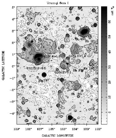
Figure 1: The gray-scale image shows the total intensity for the survey field centered at $(l,b)=(125\aas@@fstack{\circ}5,0\degr)$ with a size of $7\degr\times 10\degr$. The contours encode the total intensity with levels equal to $\pm 2^{n}\times 3\sigma_{I}$ with $n=0,1,\dots$ and $\sigma_{I}$ = 0.85 mK T_B. Solid lines show positive intensities and dotted lines negative ones.

4 Observation and processing of the first survey region

In this paper we analyse objects from the first survey region centered at $(l,b)=(125\aas@@fstack{\circ}5,0\degr)$ with a size of $7\degr\times 10\degr$. Observations for two coverages in the GL direction and two coverages in the GB direction were conducted between October 2004 and April 2006.

Following the data processing procedure described in Section 3, we obtained the total intensity map as shown in Fig. 1, the Stokes $U$ and $Q$ maps in Fig. 2 and the polarized intensity and polarization angle maps in Fig. 3. All these maps are on a relative level with the edges set to zero. Therefore the large-scale structures comparable to the map size are missed, which introduces a non-linear bias spurious for the polarization results (Reich, 2006).

4.1 Zero-level restoration

Most of the large-scale polarized emission missed in our field is probably originating from the so-called “Fan region”, which is an outstanding strong polarization feature and can be easily recognized from all existing polarization survey maps (e.g. Brouw & Spoelstra, 1976; Wolleben et al., 2006). Wilkinson & Smith (1974) and Spoelstra (1984) claimed that the “Fan region” is a local feature at a distance of about 500 pc and Faraday rotation is negligible. We assume that the “Fan region” is fully included in the 22.8 GHz (K-band) polarization map from WMAP (Page et al., 2006) which thus can be used for an estimate of missing large-scale polarization components in our $\lambda$6 cm map. We tried to compensate the missing large-scale structures in the $U$ and $Q$ maps in a similar way as described in Uyanıker et al. (1998). First, we convolved both our Urumqi $\lambda$6 cm map and the corresponding K-band $U$ and $Q$ maps to a HPBW of $2\degr$. Second, we scaled the smoothed K-band maps by the factor of $(\frac{4.8}{22.8})^{\beta}$, with a spectral index $\beta$ of $-2.8$, assuming it is the same as that for total intensities obtained by Reich & Reich (1988a, b). We note that the polarized intensity for the large-scale structures is about 300 mK in the DRAO 1.4 GHz map (Wolleben et al., 2006) and about 112 $\mu$K in the K-band map, which yields the same spectral index of about $-$2.8. Third, we subtracted the convolved Urumqi $\lambda$6 cm maps from the scaled and smoothed K-band maps to obtain the difference maps. Finally, we added the difference to the original Urumqi $U$ and $Q$ maps. Based on such zero-level restoration for $U$ and $Q$ maps, the polarized intensity and polarization angle maps were recalculated (Figs. 2 and 3). The polarized intensity of the missing large-scale structures is about 8.5 mK. As expected from the polarization angle of the “Fan region” , which is known to be around zero, the zero-level correction of the $Q$ map is large, about 8.3 mK, while that of $U$ map about $-0.6$ mK.

Original $U$

Restored $U$

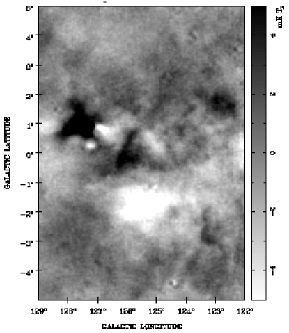
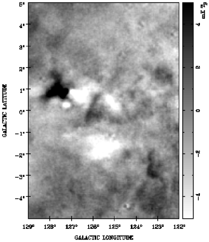
Original $Q$

Restored $Q$

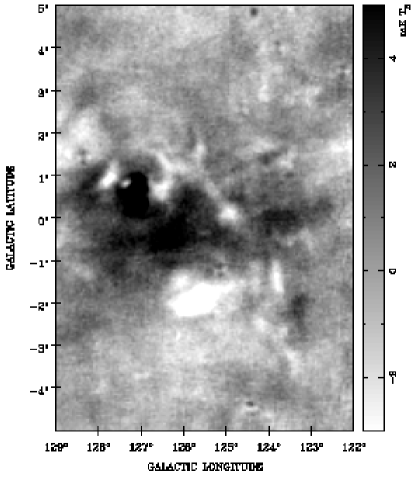
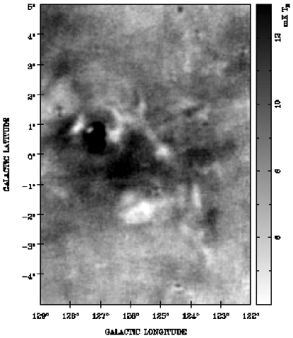
Figure 2: Gray-scale images of the original and restored $U$ and $Q$ maps.

Original PI + B-vectors

Restored PI + B-vectors

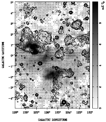
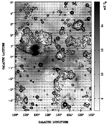
Figure 3: Gray-scale images of the polarized intensity ($PI$) with overlaid bars for every third pixels in B-field direction (polarization angle $PA+90\degr$). The length of the bars is proportional to $PI$ with a lower limit of about $\sigma_{PI}=0.4$ mK T_B. A polarized intensity of 1 mK T_B corresponds to a bar-length of 0.2 degree. Contours show total intensities with the same (positive) levels as in Fig. 1.

The $U$ and $Q$ maps with the restored large-scale structures have to be regarded as an approximation, which, however, is not too far from the real situation. Compared to the observed $U$ and $Q$ maps, the structures change dramatically after the zero-level restoration. For polarized intensity, a large-scale offset of about 8 mK has been added (Fig. 4). The most striking difference can be found in the region at $(l,b)=(125\aas@@fstack{\circ}5,-2\aas@@fstack{\circ}2)$, where the enhanced polarized intensity in the original maps is significantly reduced. The change of the polarization angle distribution is obvious from Figs. 3 and 4. The polarization angles are much less scattered when the large-scale components are included (see Fig. 4). The width of the polarization angle distribution and the mean level of polarized intensities depends on the amount of large scale emission added to the original data. Errors in the assumed spectral index used to extrapolate the WMAP polarization data towards $\lambda$6 cm have an effect on that, but the principal structure and variations are preserved compared to the original maps.

Figure 4: The distribution of polarized intensity and polarization angles before and after restoration of large-scale structures from convolved K-band $U$ and $Q$ maps as observed by WMAP (see section 4).

4.2 Accuracy and errors

The typical rms noise for total intensity, $U$ and $Q$, and polarized intensity were obtained from survey maps where the contribution from Galactic structures are nearly absent. The results are listed in Table 1.

Because the system temperature $T_{\rm sys}$ is 22 K, the bandwidth $\Delta\nu$ is 600 MHz and the integration time $\tau$ is 2 seconds, the equation $\sigma_{I}=T_{\rm sys}/\sqrt{\Delta\nu\tau}$ gives the rms noise ($\sigma_{I}$) of 0.6 mK for total intensity. This corresponds to a brightness temperature of 0.9 mK, which is calculated using the measured beam efficiency of 67%. Since $U$ and $Q$ are measured by correlating the two total intensity channels, their rms noise is lower by a factor of $\sqrt{2}$ than that of the total intensity, which means about 0.7 mK. For the first region discussed here, we have made two additional coverages with an integration time of 1.5 seconds for each and one additional coverage with standard integration time of 1 second. The theoretical rms noise is now 0.6 mK T_B for total intensity and 0.4 mK T_B for $U$ and $Q$. The measured rms noise for $I$ is 0.85 mK T_B and for $U/Q$ is 0.3 mK T_B. For polarization, the prediction is consistent with the measurements. For total intensity, the measured rms noise is slightly higher, which is likely due to limited system stability and low-level interference.

Our long-term observations of the primary survey calibrator 3C 286 (from August, 2004 to April, 2006) show that the systematic error for total intensity calibration is less than 4% and less than 5% for polarized intensity. The observations also yield the polarization angle of $32\degr\pm 1\degr$ for 3C 286, which is rather stable and very close to the assumed standard value. So we do not make further correction for the polarization angles and quote the uncertainty of the angles as 1$\degr$ for high signal-to noise ratios. We also obtained the flux density, polarization angle and polarization percentage for the secondary polarized calibrators 3C 48 and 3C 138. For 3C 48, these quantities are 5.5$\pm$0.1 Jy, $108\degr\pm 1\degr$, and (4.2$\pm$0.4)%. For 3C 138, the three quantities are 3.9$\pm$0.1 Jy, $169\degr\pm 1\degr$ and (10.8$\pm$0.5)%. The results are consistent with the values quoted in Baars et al. (1977) and Tabara & Inoue (1980). 3C 48 and 3C 138 are known for slight variations with time.

To check whether the ground radiation has been fairly removed, we compared the final map with each individual map and found that all the common structures are preserved. This means that the ground radiation, if any still remains in the results at all, is below the level of rms noise. This can result in slightly larger rms noise than theoretical prediction as shown above.

For zero-level restoration, we added just the large-scale $U$ and $Q$ components to the original maps, which do not introduce extra noise. However, the spectral index for polarized intensity is uncertain. If the spectral index varies by 0.1, the level of the restored polarized intensity will change by about 17%. This means the peak of the polarized intensity distribution after zero-level restoration (Fig. 4) will shift towards the lower or higher values. The polarization angle distribution will also change, depending how the large scale components distribute in $U$ and $Q$. For our region the missed offsets in $Q$ are much larger than in $U$. Thus spectral index errors will change the width of the angle distribution and slightly shift the mean absolute value. These shifts will, however, only slightly affect the polarization structures, and have little influence on our results on Faraday screens because our results are based on the difference or ratio between the polarized emission towards the screen and the emission in the surroundings. However, a spectral index error affects the emissivity.

5 Extended objects in the first survey region

In the first survey region we recognize a number of compact sources and extended sources or structures. A detailed analysis of compact sources will be given elsewhere (Shi et al., in preparation). Here we analyze the extended sources.

The prominent extended objects seen in the total intensity map (Fig. 1) are listed in Table 2, together with their distances - where known - and references. The objects are SNRs, HII regions or reflection nebulae. Two SNRs are identified according to the catalog of Green (2006), seven known HII regions (Sharpless HII regions and DU 65) are identified from the catalog by Sharpless (1959) and Dubois–Crillon (1976). Four so far uncatalogued objects in our map are listed at the end of the table. G128.4$+$4.3 and G122.7$+$1.5 are too weak at other bands, so we did not explore their properties further.

Polarization maps are directly related to the magnetic field structure. After adding the large-scale structures, the polarization angles are concentrated around $0\degr$ (Figs. 3 and 4), indicating a very uniform large-scale magnetic field running parallel to the Galactic plane. Some prominent features can also be recognized from the polarized intensity and B-vector maps (Fig. 3), including polarization minima and regions with polarization angles considerably deviating from the general tendency. Many of these polarized structures have no counterpart in total intensity.

The salient extended features in Figs. 1-3 are:

• SNRs G126.2$+$1.6 and G127.1$+$0.5, which have polarization detected in the relative scale maps. However the polarization towards the eastern shell of SNR G126.2$+$1.6 is considerably reduced after the zero-level restoration of $U$ and $Q$ maps.

• A polarization feature at $(l,b)=(126\aas@@fstack{\circ}2,-0\aas@@fstack{\circ}2)$ seen in the original PI map in Fig. 3, which has no correspondence in total intensity and virtually disappears in the restored map.

• The strong polarized feature at $(l,b)=(125\aas@@fstack{\circ}6,-1\aas@@fstack{\circ}8)$ seen in the original PI map without a counterpart in the total intensity map. After the restoration, the polarized intensity is slightly below that of its surroundings, however, the polarization angles remarkably deviate from the surroundings.

• The extended source G124.9$+$0.1, which shows polarization in the relative map in Fig. 3, but turns into a polarization minimum after the zero-level restoration.

• The reflection nebula Sh 185, which is probably physically connected to the shell extending towards southeastern direction. In the zero-level restored map in Fig. 3, the polarization properties towards Sh 185 are unchanged, which means that the nebula does not emit polarized emission nor depolarizes or causes Faraday rotation of the background emission.

• Polarization minima towards extended sources, such as Sh 183, are seen in both the original and the zero-level restored polarization maps, although the appearance might be patchy.

Table 2: Prominent extended objects in total intensity map at $\lambda$6 cm.

Name	$l$	$b$	$S_{4800}$	distance	Note	Ref. for distance
	($\degr$)	($\degr$)	(Jy)	(kpc)
G127.1$+$0.5	127.1	0.5	6.3$\pm$0.7	1.2, 4.4	SNR	1, 2
G126.2$+$1.6	126.2	1.6	2.6$\pm$0.6	2.4, 5.6	SNR	2, 3
DU 65	127.9	1.7		3	HII region	4
Sh 180	122.63	0.05		6.2	HII region	5
Sh 181	122.72	2.37		2.8	HII region	6
Sh 183	123.28	3.03	5.4$\pm$0.5	0.7, 6.2	HII region	6,7,13
Sh 185	123.85	$-$1.97	1.4$\pm$0.5	0.2	Reflection nebula	8, 9, 10
Sh 186	124.90	0.32		2, 3.5	HII region	11, 5
Sh 187	126.66	$-$0.79	1.2$\pm$0.1	1	HII region	12
G124.9$+$0.1	124.90	0.10	1.4$\pm$0.2	2.8	HII region	13
G124.0$+$1.4	123.95	1.40	1.6$\pm$0.3		HII region	13
G124.8$+$4.3	124.8	4.3				13
G122.7$+$1.5	122.7	1.5				13

Reference for the distance: 1. Leahy & Tian (2006); 2. Joncas, Roger & Dewdney (1989); 3. Tian & Leahy (2006); 4. Cichowolski et al. (2003); 5. Blitz, Fich & Stark (1982); 6. Fich & Blitz (1984); 7. Landecker et al. (1992); 8. Perryman et al. (1997); 9. Karr, Noriega-Crespo & Martin (2005); 10. Blouin et al. (1997); 11. Cazzolato & Pineault (2003); 12. Joncas, Durand & Roger (1992); 13. This paper.

5.1 Flux density and spectral index

To achieve an integrated net flux density of an extended source the contributions of the diffuse background and extragalactic sources must be removed. In this paper, the “background filtering” technique developed by Sofue & Reich (1979) is applied to subtract the large-scale diffuse emission. The filtering beam was taken to be $33\arcmin\times 33\arcmin$, which gives roughly the scale length of the separation between large-scale and small-scale emission. Then a ”twisted” hyper-plane fitted by using the pixel values surrounding the source is subtracted. In order to figure out the contribution from compact sources, we extracted all point sources towards the target object from the NVSS source catalog (Condon et al., 1998). The total flux density of these sources is then extrapolated to the frequency of 4.8 GHz from 1.4 GHz with a spectral index of $\alpha=-0.8$ ($S_{\nu}\propto\nu^{\alpha}$ with $S_{\nu}$ being the flux density at a frequency $\nu$) to yield the source contribution. The uncertainty of the background level and the source contribution together introduce a typical error of less than 10% of the flux density of an object.

Table 3: Spectral index $\beta$ of extended objects derived from TT-plots. Note that the CGPS 1420 MHz data include the large-scale component from the Effelsberg 1408 MHz survey. The average of $\alpha$ is also listed.

Region	radius	$\beta_{4800/1420}$		$\beta_{4800/1408}$		$\beta_{4800/865}$		$\beta_{4800/408}$		average $\alpha$		$R_{60\mu m/6cm}$
SNR G127.1$+$0.5	30′	$-$2.41$\pm$	0.01	$-$2.40$\pm$	0.01	$-$2.47$\pm$	0.03	$-$2.42$\pm$	0.01	$-$0.41$\pm$	0.02	280
SNR G126.2$+$1.6	40′	$-$2.58$\pm$	0.05	$-$2.47$\pm$	0.04	$-$2.55$\pm$	0.05	$-$2.51$\pm$	0.09	$-$0.52$\pm$	0.03	770
DU 65	24′	$-$1.91$\pm$	0.02	$-$1.91$\pm$	0.02	$-$2.07$\pm$	0.09	$-$2.01$\pm$	0.28	0.09$\pm$	0.07	440
Sh 183	27′	$-$2.02$\pm$	0.01	$-$2.06$\pm$	0.01			$-$1.90$\pm$	0.02	$-$0.02$\pm$	0.01	420
Sh 185	24′	$-$2.01$\pm$	0.06	$-$2.03$\pm$	0.07			$-$2.12$\pm$	0.14	$-$0.03$\pm$	0.06	1500
G124.9$+$0.1	27′	$-$1.97$\pm$	0.10	$-$2.01$\pm$	0.10			$-$2.15$\pm$	0.36	0.00$\pm$	0.13	1100
G124.0$+$1.4	30′	$-$2.20$\pm$	0.08	$-$2.20$\pm$	0.06			$-$2.34$\pm$	0.11	$-$0.22$\pm$	0.05	600
Sh 187	5′											5800

The spectral index can be obtained by fitting a power-law to the integrated flux densities observed at various frequencies. However, the spectral index could be influenced by the uncertainty of the background level. For example, a background level uncertainty of 10% at 4.8 GHz can introduce an error of about $-$0.1 for the spectral index between 4.8 GHz and 1.4 GHz. Therefore, we also obtained the spectral index for the brightness temperature $\beta$ via temperature-temperature plots (TT-plots), which are unaffected by the uncertainty of the background level. The flux density and brightness temperature are related via $S_{\nu}\propto\nu^{2}T_{\nu}$, so the spectral index for brightness temperatures can be translated to the spectral index for flux densities as $\alpha=\beta+2$. Fortunately many survey data are public and thus facilitates the study of TT-plots. We retrieved the CGPS 1420 MHz and 408 MHz survey data, which includes Effelsberg data for a correct representation of the large-scale emission, and also the Effelsberg 1408 MHz survey data separately. The published 865 MHz data around SNRs G127.1$+$0.5 and G126.2$+$1.6 by Reich, Zhang & Fürst (2003) were also used. We convolved all data to a common HPBW of $10\arcmin$ except for the 865 MHz data and then obtained the spectral indices $\beta$ and $\alpha$ listed in Table 3. For the spectral index between our 4800 MHz data and the 865 MHz data, we smoothed the 4800 MHz data to a HPBW of $14.5\arcmin$. Note that strong point sources have been removed before TT-plots were made.

The spectral index is an important diagnostic tool to determine the nature of an extended source. An object with a spectral index around $-$0.5 identifies that source as a SNR (Table. 3). However, a flat spectrum could originate from either a thermal source such as a HII region or a nonthermal source such as a plerion or a Crab-like SNR. The identification of a HII region can be strengthened if the exciting star can be found. Below we have intensively used the SIMBAD data base for the search of exciting stars.

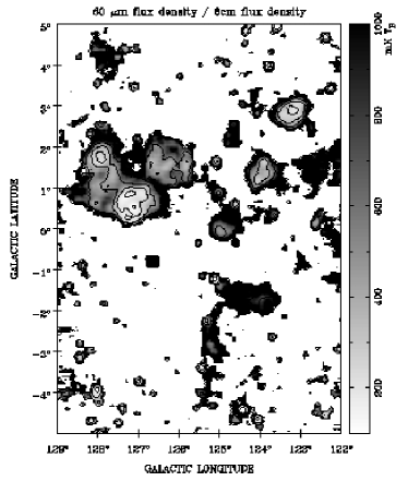
Figure 5: The ratio of the IRAS 60 $\mu$m flux density to $\lambda$6 cm flux density. The lower limit for the $\lambda$6 cm intensity is 3$\sigma_{I}$. Both maps were scaled to Jy/beam at the common beamwidth of $10\arcmin$ before the ratio was calculated. The superposed contours are at the same levels (above $3\sigma_{I}$) as in Fig. 1.

Another criterion is the ratio between the infrared flux density and the radio continuum flux density. Fürst, Reich & Sofue (1987) have reported that the ratio of the IRAS 60 $\mu$m intensity and the $\lambda$11 cm intensity $R_{\rm 60\,\mu m/11\,cm}$ is around $500\lesssim R_{\rm 60\,\mu m/11\,cm}\lesssim 1500$ for HII regions and $R_{\rm 60\,\mu m/11\,cm}\lesssim 250$ for SNRs for objects in the first Galactic quadrant. This reflects that HII regions are strong infrared emitters. Therefore we calculated the ratio $R_{\rm 60\,\mu m/6\,cm}$ to determine the nature of a source. We retrieved the high resolution IRAS 60 $\mu$m data (Cao et al., 1997) from the CGPS data archive. We scaled both the Urumqi total intensity data and the IRAS data to units of Jy/beam. The data were convolved to $10\arcmin$ and the ratio was calculated as shown in Fig. 5. The average of the ratios for some extended objects are listed in the last column of Table 3. The ratio for the SNR G127.1$+$0.5 is obviously smaller than those for the other nebulae, but that for SNR G126.2$+$1.6 is rather large, probably due to its very weak surface brightness and enhanced large-scale infrared emission in its direction. As can be seen from Fig. 5, except for the known SNRs, all extended sources all show very large ratio $R_{\rm 60\,\mu m/6\,cm}$, which indicates their thermal natures. No new SNR or plerion could be detected in the first survey region.

5.2 Interpretation of polarization structure

The observed polarization structures could be produced by two mechanisms. Synchrotron emission is intrinsically polarized, and the polarized intensity depends on the amount of the regular magnetic field component in the emitting volume. In general SNRs are polarized objects, while HII regions are not. However, as we show below, this is not necessarily directly observed in maps of polarized emission. A polarized structure can also be caused by Faraday effects within the diffuse foreground ISM or a HII region along the line of sight. The polarization in the direction of a source could be the sum of modulated background and foreground components, which can be recognized only from the zero-level restored maps.

5.2.1 The polarization of radio emission

As can be seen from Fig. 3, large-scale coherent polarized structures prevail in both the original relative and zero-level restored maps. These structures should originate either in the Perseus arm of about 2 kpc distance (Xu et al., 2006) or in the ISM up to the Perseus arm. As we show below, the polarized emission behind the Perseus arm is very weak. Beuermann, Kanbach & Berkhuijsen (1985) modeled the synchrotron emissivity of about 11 K kpc^-1 at 408 MHz. This corresponds to an emissivity of 11 mK kpc^-1 at 4.8 GHz based on a spectral index of $-$2.8. Depolarization is quite small at 4.8 GHz in case there are no Faraday screens along the line of sight. Thus the polarization percentage can be written as $p=p_{i}B_{\rm reg}^{2}/(B_{\rm reg}^{2}+B_{\rm ran}^{2})$, where $p_{i}\approx 75\%$ is the intrinsic polarization percentage, and $B_{\rm reg}$ and $B_{\rm ran}$ are the regular and random magnetic field components, respectively. Providing a distance of 2–3 kpc and a polarization percentage of about 40%, the polarized intensity is about 8.8–13.3 mK, which is consistent with the zero-level restored observations  (Fig. 3, right panel).

5.2.2 Depolarization

Depolarization can happen in three ways (Burn, 1966; Tribble, 1991; Sokoloff et al., 1998), depth depolarization, beam depolarization and bandwidth depolarization. All of them are related with the rotation measure ($RM$) and its variation $\sigma_{\rm RM}$. For depth depolarization, thermal electrons and relativistic electrons coexist within the same volume. Radio emission originating from different locations along the line of sight may have different polarization angles due to Faraday rotation, and the sum of all these Faraday rotated emission components along one line of sight will reduce the amount of observed polarization to some extent. The depolarization can be written as $DP=|\frac{1-\exp(-S)}{S}|$, where $S=2\sigma_{RM}^{2}\lambda^{4}-2i\lambda^{2}\mathcal{R}$. Here $DP$ is defined as the ratio of the observed polarized intensity to the intrinsic polarized intensity, and $\mathcal{R}$ is the RM through the entire source.

Beam depolarization occurs when the polarization angles vary across the beam, and therefore the average of the polarized emission within one beam will result in depolarization. Note that this transverse variation of $RM$ can happen both in the emission region and in the foreground medium. For the foreground case, the depolarization can be written as $DP=\exp(-2\sigma_{RM}^{2}\lambda^{4})$. Note that the $RM$ varies along the line of sight for depth depolarization but transversely to the line of sight for the beam depolarization.

The bandwidth depolarization happens when the polarization angles of the observed emission rotate significantly within the bandwidth. The depolarization $DP={\rm sinc}(2RM\lambda^{2}\frac{\Delta\nu}{\nu})$, where $\Delta\nu$ is the bandwidth of the receiving system. For our $\lambda$6 cm observations, although the bandwidth is 600 MHz, a $RM$ of around 3000 rad m^-2 is needed for total depolarization, so we consider bandwidth depolarization as not important for our survey field.

5.2.3 Faraday screens

There are lots of clumps of warm ionized medium in our Galaxy. These clumps do not emit polarization, but they impose Faraday effects on the polarization from behind. Low-density ionized gas does not show enhanced H$\alpha$ emission, but may locally show a remarkably strong regular magnetic field, as we see from the Faraday screen G125.6$-$1.8. The Faraday effects can result in: (1) rotation of the polarization angle $\psi_{\rm s}=RM_{\rm s}\lambda^{2}$, where $RM_{\rm s}$ is the RM of the screen and $\lambda$ is the observation wavelength; (2) depolarization as it has been described above. Beside the diffuse ionized gas, discrete thermal HII regions (Gaensler et al., 2001; Uyanıker et al., 2003), possibly HI clouds (Duncan et al., 1999) and the surface of molecular clouds (Wolleben & Reich, 2004) all can act as a Faraday screens. In this paper, the polarized emission originating from behind the Faraday screen is called ”background polarization” and the polarization in front of the Faraday screen is called ”foreground polarization”. The quantities are referred to as “on”, when the line of sight passes through the screen and “off” otherwise.

The “on” components of $U$ and $Q$ data can be represented in the following way,

$$\left\{\begin{array}[]{rcl}U_{\rm on}&=&PI_{\rm fg}\sin 2\psi_{\rm 0,\,fg}+fPI_{\rm bg}\sin 2(\psi_{\rm 0,\,bg}+\psi_{\rm s})\\[5.69054pt] Q_{\rm on}&=&PI_{\rm fg}\cos 2\psi_{\rm 0,\,fg}+fPI_{\rm bg}\cos 2(\psi_{\rm 0,\,bg}+\psi_{\rm s})\end{array}\right.$$ (1)

where “fg” and “bg” denote the foreground and background polarization, $f$ is the depolarization factor at 4.8 GHz, $\psi_{0}$ is the intrinsic polarization angle which does not depend on the observation frequency, and $\psi_{s}$ is the angle rotated by the Faraday screen.

As can be seen from Fig. 3, the polarization angles tend to be $0\degr$ in the restored maps, indicating that $\psi_{0,\,bg}=\psi_{0,\,fg}\approx 0\degr$. For this situation, $U_{\rm on}$ and $Q_{\rm on}$ can be simplified from Eq. (1) as,

$$\left\{\begin{array}[]{rcl}U_{\rm on}&=&fPI_{\rm bg}\sin 2\psi_{\rm s}\\[5.69054pt] Q_{\rm on}&=&PI_{\rm fg}+fPI_{\rm bg}\cos 2\psi_{\rm s}\end{array}\right.$$ (2)

Then the “on” polarized intensity ($PI_{\rm on}$) and polarization angle ($\psi_{\rm on}$) are calculated as $PI_{\rm on}=\sqrt{U^{2}_{\rm on}+Q^{2}_{\rm on}}$ and $\psi_{\rm on}=\frac{1}{2}{\rm atan}\frac{U_{\rm on}}{Q_{\rm on}}$. If the line of sight does not pass any Faraday screens, we have the “off” components as $PI_{\rm off}=PI_{\rm fg}+PI_{\rm bg}$ and $\psi_{\rm off}=0\degr$. Then the $PI$ ratio ($PI_{\rm on}$/$PI_{\rm off}$) and $PA$ difference ($\psi_{\rm on}-\psi_{\rm off}$) is obtained by,

$$\left\{\begin{array}[]{rcl}\displaystyle{\frac{PI_{\rm on}}{PI_{\rm off}}}&=&\sqrt{f^{2}(1-c)^{2}+c^{2}+2fc(1-c)\cos 2\psi_{\rm s}}\\[5.69054pt] \psi_{\rm on}-\psi_{\rm off}&=&\displaystyle{\frac{1}{2}{\rm atan}\frac{f(1-c)\sin 2\psi_{\rm s}}{c+f(1-c)\cos 2\psi_{\rm s}}}\end{array}\right.$$ (3)

where $c=PI_{\rm fg}/(PI_{\rm fg}+PI_{\rm bg})$ is the fraction of foreground polarization.

Figure 6: The $PI$ ratio ($PI_{\rm on}$/$PI_{\rm off}$) and $PA$ difference ($\psi_{\rm on}-\psi_{\rm off}$) varying with the angle rotated by the Faraday screen ($\psi_{\rm s}$) are plotted for a depolarization of $f=0.9$ and the ratio $c$ between the foreground and the total PI, $c=0.2,0.4,0.6,0.8$.

Based on Eq. (3), the $PI$ ratio and $PA$ difference are plotted for $f=0.9$ and $c=0.2,0.4,0.6,0.8$ in Fig. 6. We can see that even with very little depolarization for the background components, the $PI$ ratio can be small. We also infer that a small $PA$ difference may be caused by a large rotation angle of the Faraday screen provided with a large foreground polarization fraction (larger $c$). All this must be taken into account in any detailed analysis as discussed below.

Wolleben & Reich (2004) have proposed a similar model to fit the relations of $PI$ with $PA$, the spectral index of polarized intensity with radius and the $RM$ with radius for Faraday screens identified from the EMLS survey. In this paper, we use a model to account for the variations of the $PI$ ratio and the $PA$ difference with radius, which are independent in respect to the absolute polarization level.

5.3 Studies of individual objects

5.3.1 SNRs G126.2$+$1.6 and G127.1$+$0.5

The SNR G126.2$+$1.6 was discovered by Reich, Kallas & Steube (1979) based on its steep spectrum. Later the detection of optical emission lines and the line ratios confirmed the source as a SNR undoubtedly (Blair et al., 1980; Fesen, Gull & Ketelsen, 1983). Fürst, Reich & Steube (1984) could not rule out a spectral break at about 3 GHz. Tian & Leahy (2006) suggested a break frequency at about 1.5 GHz. These uncertainties are created by the lack of a precise flux density at $\lambda$6 cm, which was quoted as an upper limit by Fürst, Reich & Steube (1984). As we show below, the spectral curvature is ruled out using our new $\lambda$6 cm flux density.

SNR G127.1$+$0.5 was suggested to be a SNR by Pauls (1977) and Caswell (1977). The central source was originally proposed to be physically connected with the SNR like the system of SS433 in SNR W50 (Caswell, 1977; Geldzahler & Shaffer, 1982), but later it was identified as an extragalactic source by HI absorption observations  (Pauls et al., 1982; Goss & van Gorkom, 1984). A high polarization percentage of 25% at 2695 MHz and 30% at 4750 MHz were reported from the Effelsberg data (Fürst, Reich & Steube, 1984), which confirms the source as a SNR unequivocally. Optical emission from G127.1$+$0.5 was detected by Xilouris et al. (1993).

We obtained the following net flux densities: 2.6$\pm$0.6 Jy for G126.2$+$1.6 and 6.3$\pm$0.7 Jy for G127.1$+$0.5. We then revised all previous measurements by a new extragalactic source correction based on the NVSS catalog, as listed in Table 4, which ensures the consistency of the data. We note that one of the central sources 0125$+$628 in G127.1$+$0.5 is thermal and has a flat spectrum (Joncas, Roger & Dewdney, 1989; Leahy & Tian, 2006) with a flux density of 0.368 Jy at 1400 MHz from the NVSS. For this source, its flux density is taken to be 0.368 Jy at frequencies larger than 865 MHz and 0.12 Jy at 408 MHz (Joncas, Roger & Dewdney, 1989; Leahy & Tian, 2006).

Table 4: Integrated flux densities of SNRs G126.2$+$1.6 and G127.1$+$0.5 after subtraction of compact sources.

Frequency	Flux density (Jy)					Ref.
(MHz)	G126.2$+$1.6			G127.1$+$0.5
408	9.7$\pm$	3.9		16.3$\pm$	1.7	1,2
408	11.5$\pm$	2.5		16.6$\pm$	2.0	3
865	5.8$\pm$	1.6		13.6$\pm$	0.8	4
1410	5.2$\pm$	0.8		10.2$\pm$	1.2	5
1420	6.7$\pm$	2.1		9.8$\pm$	0.8	1,2
1420				9.7$\pm$	0.8	3
2695	3.9$\pm$	0.4		7.7$\pm$	0.6	5
4800	2.6$\pm$	0.6		6.3$\pm$	0.7	6
4850				5.6$\pm$	0.4	5

References: 1 Tian & Leahy (2006); 2 Leahy & Tian (2006); 3 Joncas, Roger & Dewdney (1989); 4 Reich, Zhang & Fürst (2003); 5 Fürst, Reich & Steube (1984); 6 this paper

Figure 7: The spectra of SNRs G126.2$+$1.6 (lower) and G127.1$+$0.5 (upper). The upper limit of $1.7\pm 0.2$ Jy (without source correction) for G126.2$+$1.6 at 4.85 GHz by Fürst, Reich & Steube (1984) is also marked. Our new 4.8 GHz data are indicated by filled circles.

Figure 8: TT-plots between the Urumqi 4800 MHz data and the 1420 MHz CGPS/Effelsberg data for SNRs G126.2$+$1.6 and G127.1$+$0.5.

Using the data listed in Table 4, we fitted the spectrum for both SNRs as shown in Fig. 7. The linear fit yields a spectral index of $-$0.54$\pm$0.11 for G126.2$+$1.6 and $-$0.44$\pm$0.03 for G127.1$+$0.5. It can be clearly seen from Fig. 7 (upper panel) that there is no indication of a spectral break in the frequency range from 408 MHz to 4800 MHz. The previous suggestion for a spectral curvature (Fürst, Reich & Steube, 1984; Tian & Leahy, 2006) is clearly due to the lack of a precise flux density measurement at $\lambda$6 cm.

We also checked the TT-plots between the Urumqi 4800 MHz data and the data at other frequencies. As an example, the TT-plots between our 4800 MHz data and the CGPS/Effelsberg 1420 MHz data for both SNRs are shown in Fig. 8. As can be seen from Table 3, for SNR G127.1$+$0.5 the weighted average $\alpha$ is $-$0.41$\pm$0.02 and $-$0.52$\pm$0.03 for SNR G126.2$+$1.6, both agree well with the spectral indices derived from the integrated flux densities.

Fig. 3 shows polarization towards both SNRs in the original and the zero-level restored map. SNR G127.1$+$0.5 shows strong polarization, much larger than the Galactic contribution, and the restoration process introduces just slight changes. Polarization B-vectors follow the shell, conforming to the model by van der Laan (1962). The orientation of the symmetric axis of magnetic fields is parallel to the local large-scale magnetic field, which supports the idea proposed of a barrel type SNRs by Fürst & Reich (1990). This also shows the importance of the magnetic field in shaping the evolution of SNRs.

For SNR G126.2$+$1.6 the polarization intensity is quite weak towards the eastern shell compared to its surroundings, and the orientation of the B-vectors is nearly perpendicular to the shell. Since SNR G126.2$+$1.6 is fully evolved (Tian & Leahy, 2006), this magnetic field configuration is considered as rather atypical (Fürst & Reich, 2004). This must be ascribed to the influence of the foreground or background polarization. Due to the observed $U_{\rm obs}\approx 0$ and $U_{\rm bg}=U_{\rm fg}\approx 0$, together with Eq. (2) we can obtain $\psi_{s}=0\degr$. Thus the observed $Q_{\rm obs}=Q_{\rm bg}+Q_{\rm fg}+Q_{\rm SNR}$. In the maps of original $U$ and $Q$ (Fig. 2), we see that $U_{\rm SNR}\approx 0$ and $Q_{\rm SNR}<0$. However for the background or foreground polarization, we have $U_{\rm fg/bg}\approx 0$ and $Q_{\rm fg/bg}>0$. So the addition of all the polarization will partly cancel the $Q_{\rm obs}$. Therefore the polarized intensity might get reduced, while the polarization angle is still near $0\degr$.

5.3.2 G124.9$+$0.1: a newly identified HII region

G124.9$+$0.1 is an extended source with a radius of about $27\arcmin$ and a flux density of 1.4$\pm$0.2 Jy (Fig. 9). In the original polarization map (Fig. 3), weak but distinct polarization across this extended source gives a hint for a possible SNR. However, after the restoration, a hole in polarized intensity becomes obvious, which is caused by a Faraday screen. Polarization angles inside the source deviate from those of its surroundings. The known HII region Sh 186 is located near its northern edge.

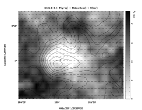
Figure 9: HII region G124.9$+$0.1: polarized intensity is gray-scale coded, H$\alpha$ intensity is shown by contours, and the orientation of the magnetic field in given by the direction of bars. The H$\alpha$ contours start at 8 Rayleigh and run in steps of 2 Rayleigh. The position of the B0 III star Hilt 102 is indicated.

The average spectral index of G124.9$+$0.1 obtained by a TT-plot is $\alpha=0.004$, confirming its thermal nature. The ratio of 60 $\mu$m flux density to 6 cm flux density (Fig. 5 and Table 3) is 1100 and consistent with HII region properties. We find a B0 III star Hilt 102 at $(l,b)=(124\aas@@fstack{\circ}95,-0\aas@@fstack{\circ}01)$, which could be the exciting star for G124.9$+$0.1 (see Fig. 9). The distance modulus of the star is 12.2 mag, what corresponds to a distance of about 2.8 kpc. We conclude that G124.9$+$0.1 is a newly identified HII region.

Thermal emission from HII regions is generated by free-free emission of electrons. The observed radio continuum emission at 4.8 GHz requires a number of ionizing photons $N_{LC}$ (Rubin, 1968; Blouin et al., 1997) as given by:

$$N_{LC}=8.825\times 10^{46}T_{4}^{-0.45}SD^{2}$$ (4)

where $N_{LC}$ is in units of s^-1, $T_{4}$ is the electron temperature in 10⁴ K, $S$ is the flux density in Jy and $D$ is the distance in kpc. Based on the radio continuum measurements at 4.8 GHz, the average electron density can be obtained by assuming a spherical model (Mezger & Henderson, 1967),

$$n_{e}=949T_{4}^{0.175}S^{0.5}D^{-0.5}\theta^{-1.5}$$ (5)

where $n_{e}$ is in units of cm^-3, $\theta$ is the apparent diameter of the source in arcmin and the other parameters are as in Eq. (4). The electron density could also be derived from the emission measure $EM$ defined as the integral of the square of electron density through the source along the line of sight. The $EM$ is related to the H$\alpha$ intensity as (Haffner, Reynolds & Tufte, 1998),

$$EM=2.75T_{4}^{0.9}I_{\rm H\alpha}\exp\left[2.44E(B-V)\right]$$ (6)

where $EM$ is in units of pc cm^-6, $I_{\rm H\alpha}$ is the H$\alpha$ intensity in Rayleigh, and $E(B-V)$ is the reddening in magnitudes.

Assuming an electron temperature of 8000 K for G124.9$+$0.1 we obtain the required $N_{LC}$ of 1.07$\times 10^{48}$ s^-1, which conforms to the value given in Panagia (1973) for a B0 III star. According to Eq. (5) we derive an electron density of 1.6 cm^-3.

We overlaid the H$\alpha$ data on the restored 4.8 GHz polarization data in Fig. 9. The H$\alpha$ data are taken from the all-sky H$\alpha$ template by Finkbeiner (2003). As can be seen from Fig. 9, there is a clear anti-correlation between the polarization intensity and the H$\alpha$ intensity. The polarization angles rotate where the H$\alpha$ emission is strong. To show their correlations, we plotted the radial distribution of these quantities. The center is selected to be located at $(l,b)=(124\aas@@fstack{\circ}90,0\aas@@fstack{\circ}05)$, the quantities are averaged within rings of $3\arcmin$-width starting from the center. According to Fig. 10, we take the radius of $27\arcmin$ as the size of the HII region. Within the source the $PA$ difference and $PI$ ratio increase gradually, while the H$\alpha$ intensity difference decreases towards larger radii. The $PI$ ratio varies from about 0.66 to nearly 1, and the $PA$ difference varies from about $-16\degr$ to about $0\degr$.

Figure 10: Variation of the difference of the H$\alpha$ intensity between “on” and “off” positions, $PA$ difference and $PI$ ratio from the center of the HII region at $(l,b)=(124\aas@@fstack{\circ}90,0\aas@@fstack{\circ}05)$ to the outskirts. The vertical dotted line marks the boundary for the “on” and “off” regions and also indicates the size of the HII region. The solid lines give a fit according to the Faraday screen model discussed in text.

We first investigate the difference of the H$\alpha$ intensity, which gives us hints for the variation of the electron density and the path length, because $I_{\rm H\alpha}\propto EM=n_{e}^{2}l$. Here $l$ is the length of the line of sight within the source. A Gaussian electron density distribution (e.g. Mezger & Henderson, 1967) and a pathlength within a spheroid could account for the observation in Fig. 10. The pathlength calculates as $l(\phi)=l_{0}\sqrt{1-\frac{D^{2}}{R^{2}}\phi^{2}}$, where $l_{0}=2R$ is the maximal pathlength passing the center, $\phi$ the offset from the center, $R$ the radius and $D$ the distance. Then the H$\alpha$ intensity can be written as $I_{\rm H\alpha}(\phi)=I_{0}e^{-\frac{\phi^{2}}{\sigma^{2}_{\rm H\alpha}}}\sqrt{1-\frac{D^{2}}{R^{2}}\phi^{2}}$ and the best fitting parameters are $I_{0}=8.5$ Rayleigh and $\sigma_{\rm H\alpha}=20\arcmin$. According to Eq. (6), the maximal H$\alpha$ intensity of 8.5 Rayleigh corresponds to an $EM$ of 260 pc cm^-6 with a reddening $E(B-V)$ of 1.07 (Hiltner, 1956). Since the $EM$ can be estimated as $2n_{e}^{2}R$, $n_{e}$ is derived as 2.3 cm^-3, which is fairly consistent with a density of 1.6 cm^-3 as estimated before.

We interpret the observed $PA$ difference and $PI$ ratio using the Faraday screen model in Eq. (3). Based on the H$\alpha$ intensity fit, we model the $PA$ rotation imposed by the Faraday screen as $\psi_{\rm s}(\phi)=\psi_{0}e^{-\frac{\phi^{2}}{\sigma^{2}_{\rm s}}}\sqrt{1-\frac{D^{2}}{R^{2}}\phi^{2}}$. Here $|\psi_{0}|$ is the maximal rotation angle. The best parameters for a reasonable fit for both the $PI$ ratio and $PA$ difference are $\psi_{0}=-50\degr$, $f=0.85$, $c=0.6$ and $\sigma_{\rm s}=18\arcmin$. The maximal rotation angle of $50\degr$ at 4.8 GHz corresponds to a maximal $RM$ of 223 rad m^-2. The maximal RM can be estimated as $RM=2Kn_{e}B_{||}R$, where $K=0.81$ is a constant. With a distance of about 2.8 kpc and a radius of 27′, we obtain about 22 pc for $R$. $n_{e}$ was taken to be 1.6 cm^-3. We obtain a magnetic field component along the line of sight of $B_{||}\approx 3.9\leavevmode\nobreak\ \mu$G, which is consistent with the magnetic field strength derived for other HII regions based on excessive RMs of extragalactic sources observed in their direction (Heiles, Chu & Troland, 1981).

As can be seen from Fig. 10, the fit for the $PI$ ratio is roughly fine but not exact. A depolarization factor $f\approx 1$ is needed to fit solely the $PI$ ratio, which means that the Faraday screen does not depolarize the background polarization. It could be that there exist an extended envelope around the HII region, which causes an underestimation of the rotation angle ($\psi_{\rm s}$) of the screen by several degrees. But this does not affect the $PI$ ratio, which is nearly constant for small $\psi_{\rm s}$ as can be seen from Fig. 6.

The fitting above also gives a foreground polarization of about 7 mK, which allows us estimate the emissivity of the synchrotron emission in this direction. For a distance of 2.8 kpc we calculate an emissivity for the polarized intensity of 2.5 mK kpc^-1. Assuming a polarization percentage of about 40%, we got the emissivity for total intensity of 6.3 mK kpc^-1 at 4.8 GHz, corresponding to an emissivity at 22 MHz of about 22 K pc^-1 for a spectral index of $-$2.8 and about 7.6 K pc^-1 for a spectral index of $-$2.6. Roger et al. (1999) reported a synchrotron emissivity of 20.9 K pc^-1 obtained using the absorption towards the nearby HII region IC 1805 with a distance of 2.2 kpc located at $(l,b)=(134\aas@@fstack{\circ}8,0\aas@@fstack{\circ}9)$ at 22 MHz. All results are consistent with a spectral index of $-$2.8.

5.3.3 An extended shell emerging from Sh 185

The nebula Sh 185 contains two reflection nebulae IC 63 and IC 59 (Blouin et al., 1997), which could be marginally resolved by our observation. The total flux density of Sh 185 at 6 cm is 1.4$\pm$0.5 Jy. The complex is illuminated by the B0 IV star $\gamma$ Cas at a distance of 190 pc (Perryman et al., 1997).

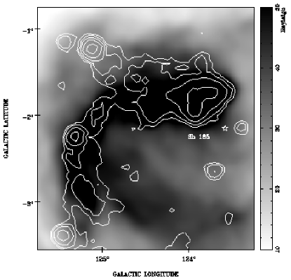
Figure 11: The total intensity at 6 cm of Sh 185 is shown in contours with the same (positive) levels as in Fig. 1. The three point sources to the left are probably background extragalactic radio sources. The gray-scale image shows the H$\alpha$ intensity. The marked star indicates the position of $\gamma$ Cas.

The most spectacular new feature we can discern from our total intensity map at 6 cm is a shell towards south-east of Sh 185, which exactly follows the H$\alpha$ shell (Fig. 11). The radius of the Strömgren sphere of $\gamma$ Cas is 6.5 pc (Karr, Noriega-Crespo & Martin, 2005) and therefore the shell is probably illuminated by $\gamma$ Cas. Since the shell is very weak, we could only get the upper limit of about 0.5 Jy for the integrated flux density, which requires ionizing photons of $1.76\times 10^{45}$ s^-1 for an assumed temperature of the shell of 8000 K. The total ionizing photons from $\gamma$ Cas is $(5.5\pm 1.5)$$\times 10^{46}$ s^-1 (Blouin et al., 1997). From the star, the shell subtends an angle of about $25\degr$ (Fig. 11) and therefore receives the photons of about $3.85\times 10^{45}$ s^-1 from the star. This is sufficient to maintain the continuum radiation from the shell.

Sh 185 as well as the shell does not have any measureable effect at $\lambda$6 cm on the polarization observations.

Figure 12: The same ring integrated profiles as shown in Fig. 10, but for G125.6$-$1.8.

5.3.4 G125.6$-$1.8: a large Faraday screen

To the east of Sh 185 and its eastern shell, there is an outstanding region with excessive polarization centered at $(l,b)=(125\aas@@fstack{\circ}6,-1\aas@@fstack{\circ}8)$ on the original Urumqi polarization map (Fig. 3) and slightly reduced polarization after the restoration. The polarization angles are significantly modulated when compared to the surrounding angles and there is no correspondence in the total intensity map. This region has an apparent size of about 2$\aas@@fstack{\circ}$4 when fitted with a spheroid. The largest $PA$ difference at the center is about $-30\degr$, but steadily decreases towards the edge. The $PI$ ratio is nearly constant or about 90% as seen in Fig. 12, which means neither depolarization nor foreground components, i.e. $f\approx 1$. Similar to G124.9$+$0.1, we also fit the observed $PI$ ratio and $PA$ difference with the Faraday screen model in Eq. (3), and got following parameters: $\psi_{0}=-45\degr$, $\sigma_{\rm s}=36\arcmin$, $f=1$ and $c=0.4$. The maximal rotation from the Faraday screen is about $45\degr$ corresponding to a RM of about 200 rad m^-2.

The fraction of foreground polarization of 40% corresponds to a brightness temperature of about 3.6 mK. If we take the polarized emissivity of 2.5 mK kpc^-1 determined in the direction of G124.9$+$0.1, we obtain a screen distance of about 1.4 kpc. In case we use the synchrotron emissivity of 11 mK kpc^-1 extrapolated from that quoted be Beuermann, Kanbach & Berkhuijsen (1985) at 408 MHz for a spectral index of $-2.8$ and a polarization percentage of 40%, we obtain a distance of about 0.8 kpc. For further calculations we take the average of both distance estimates, about 1.1 kpc, and get about 46 pc for the screen size. The large distance also excludes the possibility that the screen is related to the local complex Sh 185, although the Faraday screen partly overlaps with the northeastern part of the Sh 185 complex.

Towards the screen, the H$\alpha$ intensity is about 30 Rayleigh (Fig. 12), which is predominantly attributed to the Sh 185 nebula. There is no indication of excessive H$\alpha$ associated to the screen at all. However, the H$\alpha$ emission from the screen might be totally masked by the nebula Sh 185. The H$\alpha$ absorption is very uncertain in the Galactic plane, therefore we cannot infer an electron density from the H$\alpha$ results.

We see no signature from this screen in the total intensity map. This means the total intensity of this object must be less than about five times the noise or 4.25 mK. The brightness temperature contributed by the screen can be represented as $T_{s}=\tau T_{e}=6n_{e}^{2}$ mK, where the opacity $\tau$ is calculated as in Rohlfs & Wilson (2000) and the electron temperature $T_{e}$ is taken as 8000 K. Since $T_{s}<4.25$ mK, we obtain the upper limit of the electron density as 0.84 cm^-3, assuming a spherical shape for the Faraday screen. This electron density corresponds to an upper limit for the H$\alpha$ intensity of about 1.3 Rayleigh for an $E(B-V)$ lower limit of 1 mag near the Galactic plane. This is beyond the detection limit in the all-sky H$\alpha$ map by Finkbeiner (2003). Together with the $RM$ derived, we obtain a lower limit for the regular magnetic field along the line of sight of 6.4 $\mu$G. This is smaller than the magnetic field strengths derived by Wolleben & Reich (2004) for a number of small Faraday screens having $\sim$2 pc in size, which are located at the edge of local molecular clouds in Taurus. However, the line of sight magnetic field component we find for G125.6$-$1.8 clearly excceds the average total field strength in the interstellar medium at this Galactocentric distance (Han et al., 2006). Faraday screens due to a thermal electron density excess and avoiding an enhanced regular magnetic field component have been discussed by Gray et al. (1998) and Uyanıker & Landecker (2002). In these two cases the distances for the objects could be not be well constrained and make such an interpretation possible. In the case of G125.6$-$1.8 an enhanced magnetic field strength seems unavoidable to be compatible with the available data.

5.3.5 Sh 183

Landecker et al. (1992) studied the radio morphology of the HII region Sh 183 using the DRAO array at 408 MHz and 1420 MHz. They proposed an so far unknown O 5.5 star for its excitation. Unfortunately we can not find any O- or B-type star towards Sh 183. The recombination and HI velocity of Sh 183 is about $-$63 km s^-1 (Landecker et al., 1992). This means a dynamical distance of about 6 kpc with the solar parameters $R_{0}=8.5$ kpc and $\Theta_{0}=220$ km s^-1. However due to the spiral shock at the leading edge of the Perseus arm (Roberts, 1972), the dynamical distance has a large error. Measurements of Cas OB7 show that the radial velocity of the gas can be displaced by about $-$20 km s^-1 due to that shock (Cazzolato & Pineault, 2003). Since Sh 183 is located at the boundary of Cas OB7, we make a similar correction and obtain a distance of about 3.6 kpc, which places Sh 183 on the far side or just behind the Perseus arm.

We determined a flux density for this HII region at 4.8 GHz of 5.3$\pm$0.5 Jy, which yields a spectral index of $-$0.05$\pm$0.05 when combined with flux densities at lower frequencies (Landecker et al., 1992). This spectral index is confirmed using the TT-plot method (Table 3).

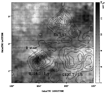
Figure 13: The same as Fig. 9 but for the region encompassing the extended ojbects Sh 183, G124.0$+$1.4 and G122.7+1.2. The H$\alpha$ intensity contours start from 10 Rayleigh and run in steps of 3 Rayleigh. A B-type star located in the center of G124.0$+$1.4 is marked.

Towards the direction of the HII region Sh 183, some weak polarization minima are visible (Fig. 13). However, the polarization angles do not differ from its surroundings, which means that the polarized emission predominately originates in the foreground in respect to Sh 183. Considering together the fact that towards the Faraday screen G124.9$+$0.1 about 80% of the polarized emission is originated within the distance of 3.6 kpc and other screen, G125.6$-$1.8, all polarized emission is originated within a distance of about 3 kpc, we conclude that the polarization emission originated behind the Perseus arm is very weak.

5.3.6 Possible new faint HII regions

The spectral index of the extended source G124.0$+$1.4 is about $-$0.22 from the TT-plots. We found a B-type star near the center of G124.0$+$1.4 (Fig. 13), which means that the source is likely a HII region. Unfortunately no further information is available for this star. The ratio of the IRAS 60 $\mu$m flux density to 4.8 GHz density (Fig. 5 and Table 3) is 660, which also suggests that this source is more likely a HII region rather than a SNR.

Other optically identified HII regions are either too weak at 6 cm (such as Sh 181 and Sh 180) or confused with complex emission regions (such as DU 65 and Sh 186), which prevents us from a more detailed study.

6 Conclusions

In this paper we report on the observation strategy and data processing procedures of the Sino-German $\lambda$6 cm continuum and polarization survey of the Galactic plane carried out with the Urumqi 25 m telescope. Preliminary results for the first survey region centered at $(l,b)=(125\aas@@fstack{\circ}5,0\degr)$ are presented.

The maps show many features in both total intensity and polarized intensity. From the total intensity maps: (1) The $\lambda$6 cm flux density of 2.6$\pm$0.6 Jy for SNR G126.2$+$1.6 was measured, which, together with previous data, rules out a spectral curvature. The integrated flux densities for other extended sources were also obtained. (2) We identified the HII region G124.9$+$0.1, being studied in some detail, and G124.0$+$1.4 being most likely also a HII-region. (3) A large thermal shell is recognized to be probably physically connected with the reflection nebula Sh 185 and being illuminated by the star $\gamma$ Cas.

We tried to compensate the so far missing large-scale structures in our $\lambda$6 cm $U$ and $Q$ maps by extrapolating WMAP K-band polarization data from 22.8 GHz to 4.8 GHz with an assumed spectral index of $-$2.8. This is to be regarded as a trial for the zero-level restoration. The polarized structures change dramatically for some regions after zero-level restoration. The polarization angles are very regular in general and trace a uniform large-scale magnetic field parallel to the Galactic plane. Some Faraday screens which show enhanced polarization in the original polarized maps are recognized after zero-level restoration. Based on model fitting for the Faraday screens, the foreground and background polarization could be separated, which allows us to assess the emissivity of the synchrotron emission. The prominent features in the polarization maps are summarized as: (1) The HII region G124.9$+$0.1 was identified as a Faraday screen in the zero-level restored maps. Its thermal electron density is estimated to be about 1.6 cm^-3 and its magnetic field component along the line of sight is about 3.9 $\mu$G. (2) Polarization is detected from SNRs G127.1$+$0.5 and G126.2$+$1.6. For the barrel type SNR G127.1$+$0.5, the magnetic field fits the direction of the Galactic large-scale magnetic field. (3) A large diameter Faraday screen G125.6$-$1.8 was identified, whose electron thermal density is estimated to be up to 0.84 cm^-3 and its magnetic field of 6.4 $\mu$G or larger.

In summary, the observations of the first region of the $\lambda$6 cm survey of the Galactic plane demonstrate their potential to detect numerous Galactic structures and to reveal new Faraday screens up to large distances, which are remarkable ISM features with strong and regular magnetic field.