How robust are inflation model and dark matter constraints from cosmological data?

Abstract

High-precision data from observation of the cosmic microwave background and the large scale structure of the universe provide very tight constraints on the effective parameters that describe cosmological inflation. Indeed, within a constrained class of $\Lambda$CDM models, the simple $\lambda\phi^{4}$ chaotic inflation model already appears to be ruled out by cosmological data. In this paper, we compute constraints on inflationary parameters within a more general framework that includes other physically motivated parameters such as a nonzero neutrino mass. We find that a strong degeneracy between the tensor-to-scalar ratio $r$ and the neutrino mass prevents $\lambda\phi^{4}$ from being excluded by present data. Reversing the argument, if $\lambda\phi^{4}$ is the correct model of inflation, it predicts a sum of neutrino masses at $0.3\to 0.5$ eV, a range compatible with present experimental limits and within the reach of the next generation of neutrino mass measurements. We also discuss the associated constraints on the dark matter density, the dark energy equation of state, and spatial curvature, and show that the allowed regions are significantly altered. Importantly, we find an allowed range of $0.094<\Omega_{c}h^{2}<0.136$ for the dark matter density, a factor of two larger than that reported in previous studies. This expanded parameter space may have implications for constraints on SUSY dark matter models.

I Introduction

The past few years have seen a dramatic increase in the precision of cosmological data, ranging from measurements of the cosmic microwave background (CMB) anisotropies by the Wilkinson Microwave Anisotropy Probe (WMAP) satellite Spergel:2006hy ; Hinshaw:2006ia ; Page:2006hz and the large scale structure (LSS) of the universe by the Sloan Digital Sky Survey (SDSS) Tegmark:2006az ; Percival:2006gt , to the observation of distant type Ia supernovae (SNIa) Astier:2005qq . All these measurements point to the so-called concordance model of cosmology, wherein the physical parameters are the baryon density $\Omega_{b}$, the matter density $\Omega_{m}$, the dark energy density $\Omega_{\Lambda}$, and the present Hubble expansion rate $H_{0}$. The model geometry is flat so that $\Omega_{\Lambda}=1-\Omega_{m}$, and the initial perturbations are assumed to be adiabatic and Gaussian, with a power law spectrum described by a spectral index $n_{s}$ and an amplitude $A_{s}$. Together with the optical depth parameter $\tau$, this six-parameter “vanilla” model provides a good fit to all observational data to date.

A common assumption in cosmological parameter estimation is that one can always improve a fit marginally by including extra free parameters. This assumption has led to the adoption by many authors of the Occam’s razor approach, in which an extra parameter is retained only if by its inclusion the goodness-of-fit of the model is substantially improved. Indeed, the success of the vanilla model is rooted in the fact that, given the current data, no addition of a single extra parameter produces a $\chi^{2}$ value that is significantly lower.

However, there are many more physically well motivated parameters beyond the vanilla model. Indeed, some of these, such as a nonzero neutrino mass, are known to be present. In such cases, a blind enforcement of Occam’s rule can lead to significant underestimation of parameter errors, as well as bias in the parameter estimates. One well-known example is the interplay between the dark energy equation of state and the neutrino mass Hannestad:2005gj ; DeLaMacorra:2006tu ; Zunckel:2006mt . When the dark energy equation of state is allowed to vary, the neutrino mass bound is relaxed by almost a factor of three if only CMB and LSS power spectrum information is used. Conversely, by imposing a prior on the neutrino masses according to the Heidelberg–Moscow claims Klapdor-Kleingrothaus:2001ke ; Klapdor-Kleingrothaus:2004wj ; VolkerKlapdor-Kleingrothaus:2005qv , reference DeLaMacorra:2006tu finds that a cosmological constant is ruled out at more than $95\ \%$ C.L. by CMB+LSS+SNIa data.

One could argue that parameter estimation coupled with Occam’s rule is a “bottom-up” approach, for which a full Bayesian analysis complete with Bayes factor calculations may also be appropriate Mukherjee:2005wg ; Parkinson:2006ku . However, if one’s aim is to exclude specific models, then a more conservative approach that takes into account possible degeneracies between the “standard” and the “new” parameters is warranted. Such a “top-down” approach does not necessarily imply a decrease in the predictability of the model. In fact, we will show that given the present cosmological data, a nonvanishing neutrino mass could be viewed as a prediction of the $\lambda\phi^{4}$ inflationary model. We argue that when constraining or excluding specific theoretical models, one should in principle allow for uncertainties in all physically well-motivated parameters, even if they have a priori no direct link to the models concerned. If, for instance, it turns out later that the universe is indeed composed of a nonvanishing neutrino fraction, it would be counterproductive to have already discarded a model of inflation that predicts this outcome.

In the present work, we investigate in this spirit how parameter constraints change when the parameter estimation analysis is performed within a much more general model framework. In principle there are some twenty or more parameters that could influence cosmology, although the precision of the present data is not yet sufficient to probe some of them (e.g., the primordial helium fraction and the effective sound speed of dark energy). Here, we focus on a 11-parameter model outlined below.

I.1 The model

We test a general 11-parameter model space consisting of

$$\Theta=(\omega_{c},\omega_{b},f_{\nu},\Omega_{k},w,H_{0},n_{s},r,\alpha_{s},\tau,A_{s}).$$ (1)

The vanilla model is defined by $f_{\nu}=\Omega_{k}=r=\alpha_{s}=0$, and $w=-1$. In addition, we marginalise over a nuisance parameter $b$ which describes the relative bias between the observed galaxy power spectrum $P_{g}(k)$ and the underlying dark matter spectrum $P_{c}(k)$ via $P_{c}(k)=b^{2}P_{g}(k)$.

Three different parameter sets will be considered in this work:

• Set A: All 11 parameters.

• Set B: A 10-parameter set with $\Omega_{k}=0$. This parameter set covers all standard inflationary models

• Set C: A 9-parameter set with $\Omega_{k}=\alpha_{s}=0$. This reduced set corresponds to the large subset of the zoo of inflationary models that predict negligible running, including large field chaotic inflation models linde .

I.1.1 Matter content

We assume the matter content to be specified by the following parameters: the curvature $\Omega_{k}=1-\Omega_{m}-\Omega_{\Lambda}$, the physical dark matter density $\omega_{c}=\Omega_{\rm c}h^{2}$, the baryon density $\omega_{b}=\Omega_{b}h^{2}$, the neutrino fraction $f_{\nu}=\Omega_{\nu}/\Omega_{c}$, and the dark energy equation of state parameter $w$.

Other parameters not included here, but which could have an observable effect, include a time-dependent dark energy equation of state, nonstandard interactions in any of the dark sectors (cold dark matter, neutrinos, or dark energy), etc. We mention this as a caution that while our parameter space is much larger than that normally used in parameter estimation analyses, it is not necessarily complete.

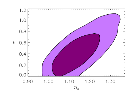
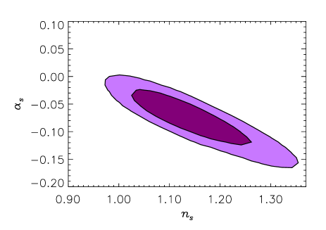
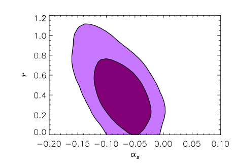
Figure 1: Two-dimensional $68\ \%$ and $95\ \%$ C.L. contours for the inflationary parameters $n_{s}$, $r$, and $\alpha_{s}$, using the full data set and parameter set B, and marginalised over the other $(10-2)$ parameters.

I.1.2 Initial conditions

The initial conditions for structure formation are assumed to be set by inflation, characterised by scalar and tensor fluctuations with amplitude $A_{s}$ and $A_{t}=rA_{s}$ respectively. Each component is specified by a spectral index $n_{s}$ or $n_{t}$, and the inflationary consistency relation requires that $n_{t}\sim-r/8$. However, the precision of current data is not yet at a level where a violation of the consistency relation can be tested. This also means that while the running parameter $\alpha_{s}$ should be included for the scalar spectrum, the inclusion of its tensor counterpart $\alpha_{t}$ would have no effect. This set of initial parameters encompasses all standard inflationary models, but not models with features from potential steps, particle production, etc. during inflation. We define $\alpha_{s}$ at the pivot scale $k=0.002$ Mpc^-1, in concordance with most recent analyses.

Note that an alternative approach would be to perform the analysis directly in terms of the slow-roll parameters instead of the observables $n_{s}$, $\alpha_{s}$, and $r$ Leach:2003us ; Peiris:2006ug ; Peiris:2006sj . Particularly for models where $\alpha_{s}$ is not negligible this can lead to somewhat different results. However, in models with small $\alpha_{s}$, such as chaotic inflation, the results are identical.

II Data analysis

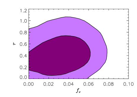
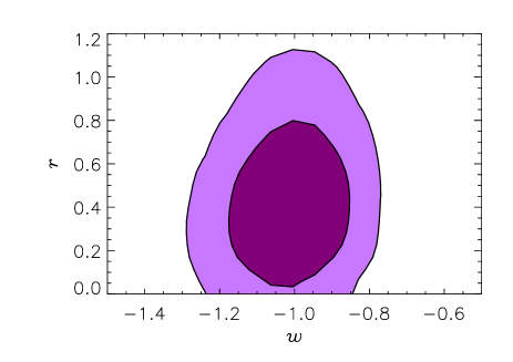
Figure 2: Degeneracies between $r$ and $f_{\nu},w$ for the full data set and parameter set B, marginalised over $(10-2)$ parameters.

Cosmic microwave background (CMB)  We use CMB data from the WMAP experiment after three years of observation Spergel:2006hy ; Hinshaw:2006ia ; Page:2006hz . The data analysis is performed using the likelihood calculation package provided by the WMAP team on the LAMBDA homepage lambda .

Large scale structure (LSS)  The large scale structure power spectrum of luminous red galaxies (LRG) has been measured by the Sloan Digital Sky Survey (SDSS). We use the same analysis technique on this data set as advocated by the SDSS team Tegmark:2006az ; Percival:2006gt , with analytic marginalisation over the bias $b$ and the nonlinear correction parameter $Q_{\rm nl}$.

Baryon acoustic oscillations (BAO)  In addition to the power spectrum data we use the measurement of baryon acoustic oscillations in the two-point correlation function Eisenstein2005 . The analysis is performed following the procedure described in Eisenstein2005 ; Eisensteinweb (see also Goobar:2006xz ), including analytic marginalisation over the bias $b$, and nonlinear corrections with the HALOFIT halofit package.

Type Ia supernovae (SNIa)  We use the luminosity distance measurements of distant type Ia supernovae provided by the Supernova Legacy Survey (SNLS) Astier:2005qq .

Lyman-$\alpha$ forest  We do not include data from the Lyman-$\alpha$ forest in our analysis. These data were used in some previous studies that found very strong bounds on various cosmological parameters seljak2006 . However, the strength of these bounds is due mainly to the fact that the Lyman-$\alpha$ analysis used in seljak2006 leads to a much higher normalisation of the small-scale power spectrum than that obtained from the WMAP data. Other analyses of the same SDSS Lyman-$\alpha$ data find a lower normalisation, in better agreement with the WMAP result Viel:2005eg ; Viel:2005ha ; viel2006 . This kind of discrepancy between different analyses of the same data probably points to unresolved systematic issues, and for this reason we prefer to discard the Lyman-$\alpha$ data entirely.

For a large part of our analysis we use two different combinations of data sets, one consisting of WMAP and SDSS data only, and one which uses in addition data from SNIa (SNLS) and BAO. The latter case is sometimes referred to as “the full data set”.

We perform the data analysis using the publicly available CosmoMC package Lewis:2002ah ; cosmomc , modified to include the BAO likelihood calculations.

Table 1: The $95\ \%$ C.L. allowed ranges for $n_{s}$, $r$ and $\alpha_{s}$ for parameter set B, marginalised over the other $(10-1)$ parameters.

Parameter	WMAP+SDSS	Full data set
$n_{s}$	$0.97\to 1.35$	$0.98\to 1.28$
$r$	$0\to 1.05$	$0\to 0.81$
$\alpha_{s}$	$-0.140\to-0.005$	$-0.135\to-0.004$

III Results

III.1 Inflationary parameters

Almost all inflationary models predict $\Omega_{k}$ to be zero. This prediction is also supported by our analysis of parameter set A (see Sec. III.4). Therefore, in this section, we will work with the reduced 10-parameter set B, in which $\Omega_{k}$ is already fixed at zero. Figure 1 shows the 2D likelihood contours for the parameters $n_{s},r$ and $\alpha_{s}$ using the full data set and parameter set B. These contours are obtained by marginalising over the other $(10-2)$ parameters not shown in the plot.

Figure 1 should be compared with, e.g., Figs. 2 and 3 of Kinney et al. Kinney:2006qm , which use data from WMAP and SDSS, and a parameter set similar to our set B but with $f_{\nu}$ and $w$ fixed at $0$ and $-1$ respectively. The comparison reveals that the two sets of likelihood contours are roughly similar, but with one important exception: the allowed range for the tensor-to-scalar ratio $r$ in our case is much larger even in the light of additional data!

In order to understand this effect we plot in Fig. 2 the 2D likelihood contours for $r$ and our additional parameters $f_{\nu}$ and $w$. Interestingly, a substantial degeneracy exists between $r$ and the neutrino fraction $f_{\nu}$, which in turn allows $r$ to extend to much higher values. Table 1 displays the 1D $95\ \%$ C.L. allowed ranges for $n_{s}$, $r$, and $\alpha_{s}$, assuming parameter set B and using both WMAP+SDSS only and the full data set.

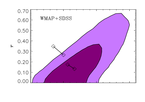
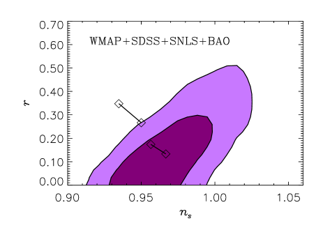
Figure 3: Two-dimensional $68\ \%$ and $95\ \%$ C.L. contours for $n_{s}$ and $r$, using parameter set C (consistent with predictions of chaotic inflation), and marginalised over $(9-2)$ parameters. The upper panel uses WMAP+SDSS data and the lower the full data set. The two short black/solid lines with boxes at the ends correspond to predictions of $\lambda\phi^{4}$ (top left) and $m^{2}\phi^{2}$ models of inflation, with 46 to 60 $e$-foldings (left to right).

III.2 Chaotic inflation

Single field inflation models with polynomial potentials generally predict negligible running. These models are thus represented by our 9-parameter set C in which $\alpha_{s}=0$. The corresponding 2D likelihood contours for $n_{s}$ and $r$, marginalised over the other $(9-2)$ parameters, are shown in Fig. 3.

Table 2: The 1D marginalised $95\ \%$ C.L. allowed ranges for $n_{s}$ and $r$ for parameter set C and its subsets.

Parameter set	Data set	$n_{s}$	$r$
C	WMAP+SDSS	$0.927\to 1.038$	$0\to 0.51$
C	WMAP+SDSS+SNLS+BAO	$0.932\to 1.018$	$0\to 0.41$
C	WMAP+SDSSlin+SNLS+BAO	$0.931\to 1.025$	$0\to 0.47$
C, $w$ fixed	WMAP+SDSS+SNLS+BAO	$0.933\to 1.019$	$0\to 0.40$
C, $w,f_{\nu}$ fixed	WMAP+SDSS	$0.931\to 1.011$	$0\to 0.31$
C, $w,f_{\nu}$ fixed	WMAP+SDSS+SNLS+BAO	$0.931\to 1.010$	$0\to 0.30$

Figure 3 should be compared with Fig. 4 of Kinney et al. Kinney:2006qm , with Fig. 14 of Spergel et al. Spergel:2006hy , and with Fig. 19 of Tegmark et al. Tegmark:2006az (see also Martin:2006rs ). In all cases our WMAP+SDSS contours encompass a markedly larger region. In particular, even with the inclusion of SNIa and BAO data, we find that the simplest $\lambda\phi^{4}$ model is still allowed by data, contrary to the conclusions of Kinney:2006qm ; Spergel:2006hy ; Tegmark:2006az ; Martin:2006rs . We note that the endpoints of the model lines in Fig. 3 correspond to 46 and 60 e-foldings respectively. Interestingly, $\lambda\phi^{4}$ is compatible with data only if the number of $e$-foldings is relatively large, or equivalently, if the reheating temperature is high dodelson ; Liddle:2003as .

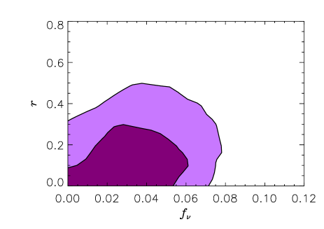
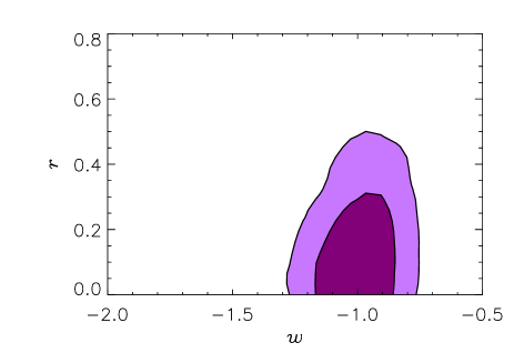
Figure 4: Degeneracies between between $r$ and $f_{\nu},w$ for the full data set and parameter set C, marginalised over $(9-2)$ parameters.

Again, the explanation for our enlarged $n_{s},r$ allowed region lies in our expanded model parameter space. In Fig. 4, we see that the degeneracy between $r$ and $f_{\nu}$ encountered earlier in parameter set B is present also in parameter set C, albeit to a smaller extent. If a neutrino fraction of $0.03\to 0.05$ is allowed (corresponding roughly to $\sum m_{\nu}\sim 0.3\to 0.5$ eV), new parameter space opens up for $n_{s}$ and $r$. We note in passing that the converse is not true. Allowing $r$ to run does not change the upper bound on the neutrino mass significantly. Interestingly, this $f_{\nu},r$ degeneracy also means that $\lambda\phi^{4}$ in its simplest form predicts quasi-degenerate neutrino masses with a sum in the $0.3\to 0.5$ eV range. This range is compatible with present laboratory limits from tritium beta decay experiments, $m_{\nu}<2.2\ {\rm eV}$ Lobashev:2003kt ; Kraus:2004zw , as well as the claimed detection of neutrinoless double beta decay, and hence detection of the effective electron neutrino mass $m_{ee}=\left|\sum_{j}U^{2}_{ej}m_{\nu_{j}}\right|$ at $0.1\to 0.9$ eV , by the Heidelberg–Moscow experiment Klapdor-Kleingrothaus:2001ke ; Klapdor-Kleingrothaus:2004wj ; VolkerKlapdor-Kleingrothaus:2005qv . The upcoming tritium beta decay experiment KATRIN will also probe neutrino masses to a comparable level of precision katrin .

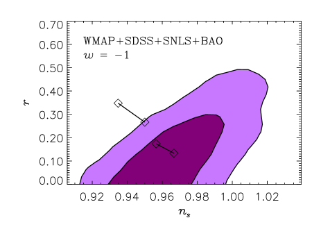
Figure 5: Two-dimensional marginalised constraints on $n_{s}$ and $r$ for the parameter set C, but with the restriction $w=-1$.

Also of interest is the case of a fixed dark energy equation of state $w$. Figure 5 shows the equivalent of the lower panel of Fig. 3 (full data set and parameter set C), but with the additional restriction $w=-1$. Clearly, there is very little difference between Figs. 3 and 5, since the combination of SNIa and BAO data effectively fixes $w$ to $-1$ in the former case, as shown in Fig. 4.

As a consistency check we present in Fig. 6 also the 2D constraints on $n_{s},r$ for the vanilla model with one extra parameter $r$, i.e., the same model analysed in Kinney:2006qm ; Spergel:2006hy ; Tegmark:2006az . The general shapes of the contours in this figure are almost identical to those in Fig. 19 in Tegmark et al. Tegmark:2006az which uses the same data sets. In addition, we find a 1D $95\ \%$ C.L. upper bound of $r<0.31$, while Tegmark et al. report an almost identical $r<0.33$. Kinney et al. also found $r<0.31$ for the same vanilla+$r$ model Kinney:2006qm , but from a combination of WMAP and the SDSS main galaxy samples (as opposed to SDSS LRG used in this work and in Tegmark:2006az ). For comparison finelli found $r<0.26$ for an analysis of WMAP and 2dF.

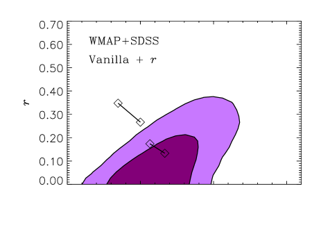
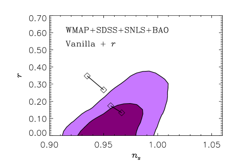
Figure 6: Two-dimensional marginalised contours for the vanilla+$r$ parameter space, for both WMAP+SDSS only (upper panel) and the full data set (lower panel).

Using additional data from the Lyman-$\alpha$ forest, Seljak et al. seljak2006 derived an even stronger upper bound, $r<0.22$, for the same model space. The reason for the improvement is a degeneracy between $r$ and $\sigma_{8}$, such that a higher value of $r$ leads to a smaller preferred value of $\sigma_{8}$. Since the Lyman-$\alpha$ data used in seljak2006 prefer a high value of $\sigma_{8}$, a small $r$ value is correspondingly favoured. In fact, from a parameter fitting point of view, a negative $r$ would be even better. All these conspire to give a much stronger upper bound on $r$. However, as noted in Sec. II, this phenomenon likely points to a systematic uncertainty in the Lyman-$\alpha$ normalisation, rather than a genuinely strong constraint on $r$.

Finally, we stress again that the difference between the allowed $n_{s},r$ regions in Figs. 3 and 6 lies in a degeneracy between $r$ and the neutrino fraction $f_{\nu}$. It should also be noted that the addition of SNIa and BAO data has very little impact on the vanilla+$r$ model, because no strong parameter degeneracies are present in the WMAP+SDSS data. With SNIa and BAO included we find a 1D $95\ \%$ C.L. bound of $r<0.30$, instead of $0.31$ for WMAP+SDSS alone.

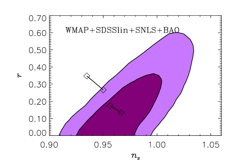
Figure 7: Two-dimensional marginalised constraints on $n_{s}$ and $r$ for parameter set C. Only the linear part of the SDSS power spectrum has been used.

III.3 The effect of non-linearity

So far we have used exactly the same analysis technique as the SDSS team when treating the LRG data. However, beyond a wavenumber of approximately $k\sim 0.06\to 0.07\ h\ {\rm Mpc}^{-1}$, nonlinear effects begin to dominate the matter spectrum (see, for instance, Fig. 9 of Tegmark:2006az ). To test whether or not our results are subject to these effects, we perform the same analysis as in Fig. 3, but retain data only up to $k\sim 0.06\ h\ {\rm Mpc}^{-1}$ (band 11). We call this reduced data set SDSSlin, and the result is shown in Fig. 7. Using only the linear part of the power spectrum data has no bearing on our conclusions. In fact, the 2D allowed region in $n_{s},r$ for parameter set C is only affected in the region where $n_{s}>1$. The SDSS data probes $n_{s}$ more precisely when all data points are included, and this in turn leads to a truncation of the allowed region at high $n_{s}$.

Table 2 summarises the 1D marginalised constraints on $n_{s}$ and $r$ for parameter set C and its subsets.

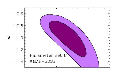
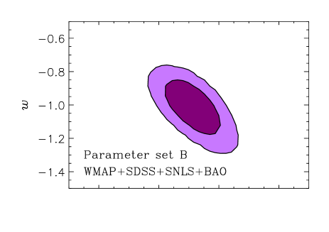
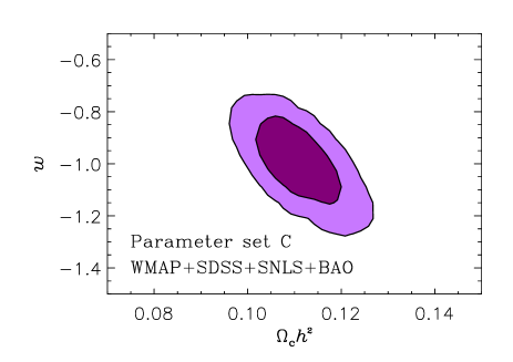
Figure 8: Two-dimensional marginalised $68\ \%$ and $95\ \%$ C.L. contours for $\Omega_{c}h^{2}$ and $w$, using various parameter and data sets. Top: Parameter set B, WMAP+SDSS. Middle: Parameter set B, the full data set. Bottom: Parameter set B with $\alpha_{s}=0$ (i.e., parameter set C), the full data set.

III.4 Dark matter and dark energy

In order to derive robust bounds on the physical dark matter and dark energy properties, all other plausible parameters should be allowed to vary. With respect to the initial conditions this is almost impossible since the most general inflationary models do not necessarily give smooth, power law-like spectra. Instead, the primordial power spectrum can have various features Starobinsky:1986fx ; Adams:1997de ; Elgaroy:2003hp ; Hunt:2004vt ; Covi:2006ci ; Martin:2003kp ; Contaldi:2003zv (see also Souradeep:1997my ; Wang:1998gb ; Hannestad:2000pm ; Hannestad:2003zs ; Bridges:2006zm ; Shafieloo:2006hs for more observationally oriented discussions), which may bias estimates of parameters and their errors. Here we present just a small step towards dark matter and dark energy parameter estimation in the context of more general models.

The physical dark matter density $\Omega_{c}h^{2}$ is a crucial input in dark matter model building. A prime example of this is models with low energy SUSY where the dark matter particle is usually either the neutralino or the gravitino. Large regions in parameter space in these models have been excluded by the fact that the predicted dark matter density is too high or too low Profumo:2004at ; deAustri:2006pe ; Ellis:2003si ; Battaglia:2003ab ; Ellis:2003cw ; Carena:2006nv ; Baltz:2006fm ; Aguilar-Saavedra:2005pw ; Belanger:2005jk ; Allanach:2004xn ; Steffen:2006hw .

In the vanilla model $\Omega_{c}h^{2}$ is a very well constrained quantity, with WMAP+SDSS giving a $68\ \%$ C.L. limit of $\Omega_{c}h^{2}=0.1050^{+0.0041}_{-0.0040}$ Tegmark:2006az . This corresponds to a relative uncertainty of $\sigma(\Omega_{c}h^{2})/\Omega_{c}h^{2}\simeq 0.04$. The SDSS collaboration also provide bounds on $\Omega_{c}h^{2}$ in extended models in which one additional parameter is added to the vanilla parameter set Tegmark:2006az . In most cases the bound on $\Omega_{c}h^{2}$ does not change significantly. However, when either $\Omega_{k}$ or $w$ is allowed to vary, $\sigma(\Omega_{c}h^{2})/\Omega_{c}h^{2}$ increases to about $0.06$ Tegmark:2006az .

We have taken this investigation further by calculating the bound on $\Omega_{c}h^{2}$ for our various parameter and data sets. In Fig. 8 we show the joint 2D marginalised constraints on $\Omega_{c}h^{2}$ and $w$ for three different cases using parameter sets B and C. If only WMAP and SDSS data are used, a very strong degeneracy between $\Omega_{c}h^{2}$ and $w$ weakens the bounds on both parameters. This degeneracy is broken when SNIa and BAO are included (as is also the case with the degeneracy between $f_{\nu}$ and $w$), yielding strong constraints on both parameters.

When spatial curvature is also allowed to vary, the bound on $\Omega_{c}h^{2}$ does change considerably. Figure 9 shows the 2D marginalised contours for $\Omega_{c}h^{2},\Omega_{k}$ and $w$, using parameter set A and the full data set. Here we find $\sigma(\Omega_{c}h^{2})/\Omega_{c}h^{2}\simeq 0.1$, so that $0.094<\Omega_{c}h^{2}<0.136$, $-0.022<\Omega_{k}<0.026$, and $-1.19<w<-0.88$ (1D at $95\ \%$ C.L.). It is interesting to compare our more general constraints on $\Omega_{k}$ with that given by the SDSS collaboration from a vanilla+$\Omega_{k}$ fit ($-0.015<\Omega_{k}<0.023$, $95\ \%$ C.L.) Tegmark:2006az ; our allowed range is slightly larger even in the light of additional data from the distance measurements of SNIa and BAO. We note also that even though the allowed range for $\Omega_{c}h^{2}$ increases considerable with the inclusion of $\Omega_{k}$, the same is not true for the dark energy equation of state parameter $w$. In Table 3, we summarise the 1D $95\ \%$ constraints on $\Omega_{c}h^{2}$ and $w$ from Figs. 8 and 9

Finally, let us we stress that some caution should be applied whenever the dark matter density is used as an input to constrain models such as the MSSM. Parameter regions that are excluded in the simplest vanilla model can easily be allowed in more general models, even without the introduction of more exotic features such as isocurvature modes. If one is to take one single number inferred from cosmological observations as an input to constrain particle physics models, then the safest approach is to allow for the possibility that cosmology is not described by the vanilla model, but by something more general. From our calculations, we recommend using $0.094<\Omega_{c}h^{2}<0.136$ ($95\ \%$ C.L.), but we caution that even this may not be the most conservative estimate.

Table 3: The 1D marginalised $95\ \%$ C.L. allowed ranges for $\Omega_{c}h^{2}$ and $w$ for various parameter and data sets.

Parameter set	Data set	$\Omega_{c}h^{2}$	$w$
B	WMAP+SDSS	$0.092\to 0.136$	$-1.44\to-0.76$
B	WMAP+SDSS+SNLS+BAO	$0.100\to 0.123$	$-1.12\to-0.87$
C	WMAP+SDSS+SNLS+BAO	$0.100\to 0.123$	$-1.11\to-0.86$
A	WMAP+SDSS+SNLS+BAO	$0.094\to 0.136$	$-1.19\to-0.88$

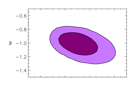
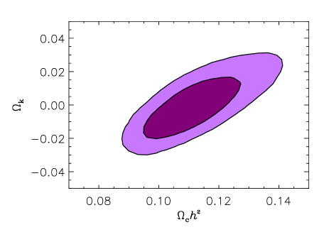
Figure 9: Two-dimensional marginalised $68\ \%$ and $95\ \%$ C.L. contours for $\Omega_{c}h^{2}$, $\Omega_{k}$, and $w$, using parameter set A and the full data set.

IV Discussion

We have performed a detailed study of cosmological parameter estimation in the context of extended models that encompass a larger model parameter space than the standard, flat $\Lambda$CDM cosmology. Using the 6-parameter vanilla model as a basis, we include as additional parameters only those that are physically motivated, such as a nonzero neutrino mass. We consider a 11-parameter model and subsets thereof, in contrast with the vanilla+1 approach adopted in most previous analyses which treats one extra parameter at a time.

In this more general framework, we find that in the context of standard slow-roll inflation, constraints on the dark matter and dark energy parameters can be substantially altered. If only CMB and LSS data are used, the larger parameter space introduces new, strong parameter degeneracies, e.g., between the physical dark matter density $\Omega_{c}h^{2}$ and the dark energy equation of state $w$. These degeneracies can be broken to a large extent by adding type Ia supernova and baryon acoustic oscillation data to the analysis. However, even with this expanded data set, we find that the bound on the physical dark matter density $\Omega_{c}h^{2}$ relaxes by more than a factor of two compared to the vanilla model constraint.

In the same spirit, we have studied how bounds on the inflationary parameters $n_{s}$, $r$, and $\alpha_{s}$ are affected by the introduction of extra parameters in the analysis. We find that the simplest $\lambda\phi^{4}$ model of inflation is still compatible with all present data at the $95\ \%$ level, in contrast with other recent analyses Kinney:2006qm ; Spergel:2006hy ; Tegmark:2006az . The source of this apparent discrepancy is a strong degeneracy between the tensor-to-scalar ratio $r$ and the neutrino fraction $f_{\nu}$, the latter of which was fixed at zero in the analyses of Kinney:2006qm ; Spergel:2006hy ; Tegmark:2006az . Reversing the argument, if $\lambda\phi^{4}$ is the true model of inflation, then it strongly favours a sum of quasi-degenerate neutrino masses between $0.3$ and $0.5$ eV, a range compatible with present data from laboratory experiments. This represents a clear example of how neutrino masses well within laboratory limits can bias conclusions about other, seemingly unrelated cosmological parameters.

References

- (1) D. N. Spergel et al., arXiv:astro-ph/0603449.
- (2) G. Hinshaw et al., arXiv:astro-ph/0603451.
- (3) L. Page et al., arXiv:astro-ph/0603450.
- (4) M. Tegmark et al., arXiv:astro-ph/0608632.
- (5) W. J. Percival et al., arXiv:astro-ph/0608636.
- (6) P. Astier et al., Astron. Astrophys. 447, 31 (2006) [arXiv:astro-ph/0510447].
- (7) S. Hannestad, Phys. Rev. Lett. 95, 221301 (2005) [arXiv: astro-ph/0505551].
- (8) A. De La Macorra, A. Melchiorri, P. Serra and R. Bean, arXiv:astro-ph/0608351.
- (9) C. Zunckel and P. G. Ferreira, arXiv:astro-ph/0610597.
- (10) H. V. Klapdor-Kleingrothaus, A. Dietz, H. L. Harney and I. V. Krivosheina, Mod. Phys. Lett. A 16, 2409 (2001) [arXiv:hep-ph/0201231].
- (11) H. V. Klapdor-Kleingrothaus, I. V. Krivosheina, A. Dietz and O. Chkvorets, Phys. Lett. B 586, 198 (2004) [arXiv:hep-ph/0404088].
- (12) H. V. Klapdor-Kleingrothaus, arXiv:hep-ph/0512263.
- (13) P. Mukherjee, D. Parkinson and A. R. Liddle, Astrophys. J. 638, L51 (2006) [arXiv:astro-ph/0508461].
- (14) D. Parkinson, P. Mukherjee and A. R. Liddle, Phys. Rev. D 73, 123523 (2006) [arXiv:astro-ph/0605003].
- (15) S. M. Leach and A. R. Liddle, Phys. Rev. D 68, 123508 (2003) [arXiv:astro-ph/0306305].
- (16) H. Peiris and R. Easther, JCAP 0607, 002 (2006) [arXiv:astro-ph/0603587].
- (17) H. Peiris and R. Easther, JCAP 0610, 017 (2006) [arXiv:astro-ph/0609003].
- (18) A. D. Linde, Phys. Lett. B 129, 177 (1983).
- (19) http://lambda.gsfc.nasa.gov
- (20) D. J. Eisenstein et al. [SDSS Collaboration], Astrophys. J. 633, 560 (2005) [arXiv:astro-ph/0501171].
- (21) http://cmb.as.arizona.edu/eisenste/acousticpeak
- (22) A. Goobar, S. Hannestad, E. Mortsell and H. Tu, JCAP 0606, 019 (2006) [arXiv:astro-ph/0602155].
- (23) R. E. Smith et al. [The Virgo Consortium Collaboration], Mon. Not. Roy. Astron. Soc. 341, 1311 (2003) [arXiv:astro-ph/0207664].
- (24) U. Seljak, A. Slosar and P. McDonald, JCAP 0610, 014 (2006) [arXiv:astro-ph/0604335].
- (25) M. Viel, M. G. Haehnelt and V. Springel, Mon. Not. Roy. Astron. Soc. 367, 1655 (2006) [astro-ph/0504641].
- (26) M. Viel and M. G. Haehnelt, Mon. Not. Roy. Astron. Soc. 365, 231 (2006) [astro-ph/0508177].
- (27) M. Viel, M. G. Haehnelt and A. Lewis, astro-ph/0604310.
- (28) A. Lewis and S. Bridle, Phys. Rev. D 66, 103511 (2002) [arXiv:astro-ph/0205436].
- (29) http://cosmologist.info
- (30) W. H. Kinney, E. W. Kolb, A. Melchiorri and A. Riotto, Phys. Rev. D 74, 023502 (2006) [arXiv:astro-ph/0605338].
- (31) J. Martin and C. Ringeval, JCAP 0608, 009 (2006) [arXiv:astro-ph/0605367].
- (32) M. S. Sloth, Nucl. Phys. B 748, 149 (2006) [arXiv:astro-ph/0604488].
- (33) S. Dodelson and L. Hui, Phys. Rev. Lett. 91, 131301 (2003) [arXiv:astro-ph/0305113].
- (34) A. R. Liddle and S. M. Leach, Phys. Rev. D 68, 103503 (2003) [arXiv:astro-ph/0305263].
- (35) V. M. Lobashev, Nucl. Phys. A 719, 153 (2003).
- (36) C. Kraus et al., Eur. Phys. J. C 40, 447 (2005) [arXiv: hep-ex/0412056].
- (37) G. Drexlin [KATRIN Collaboration], Nucl. Phys. Proc. Suppl. 145, 263 (2005).
- (38) F. Finelli, M. Rianna and N. Mandolesi, arXiv:astro-ph/0608277.
- (39) A. A. Starobinsky, JETP Lett. 42, 152 (1985) [Pisma Zh. Eksp. Teor. Fiz. 42, 124 (1985)].
- (40) J. A. Adams, G. G. Ross and S. Sarkar, Nucl. Phys. B 503, 405 (1997) [arXiv:hep-ph/9704286].
- (41) O. Elgaroy, S. Hannestad and T. Haugboelle, JCAP 0309, 008 (2003) [arXiv:astro-ph/0306229].
- (42) P. Hunt and S. Sarkar, Phys. Rev. D 70, 103518 (2004) [arXiv:astro-ph/0408138].
- (43) L. Covi, J. Hamann, A. Melchiorri, A. Slosar and I. Sorbera, Phys. Rev. D 74, 083509 (2006) [arXiv:astro-ph/0606452].
- (44) J. Martin and R. Brandenberger, Phys. Rev. D 68, 063513 (2003) [arXiv:hep-th/0305161].
- (45) C. R. Contaldi, M. Peloso, L. Kofman and A. Linde, JCAP 0307, 002 (2003) [arXiv:astro-ph/0303636].
- (46) T. Souradeep, J. R. Bond, L. Knox, G. Efstathiou and M. S. Turner, arXiv:astro-ph/9802262.
- (47) Y. Wang, D. N. Spergel and M. A. Strauss, Astrophys. J. 510, 20 (1999) [arXiv:astro-ph/9802231].
- (48) S. Hannestad, Phys. Rev. D 63, 043009 (2001) [arXiv: astro-ph/0009296].
- (49) S. Hannestad, JCAP 0404, 002 (2004) [arXiv:astro-ph/0311491].
- (50) M. Bridges, A. N. Lasenby and M. P. Hobson, arXiv: astro-ph/0607404.
- (51) A. Shafieloo, T. Souradeep, P. Manimaran, P. K. Panigrahi and R. Rangarajan, arXiv:astro-ph/0611352.
- (52) S. Profumo and C. E. Yaguna, Phys. Rev. D 70, 095004 (2004) [arXiv:hep-ph/0407036].
- (53) R. R. de Austri, R. Trotta and L. Roszkowski, JHEP 0605, 002 (2006) [arXiv:hep-ph/0602028].
- (54) J. R. Ellis, K. A. Olive, Y. Santoso and V. C. Spanos, Phys. Rev. D 69, 095004 (2004) [arXiv:hep-ph/0310356].
- (55) M. Battaglia, A. De Roeck, J. R. Ellis, F. Gianotti, K. A. Olive and L. Pape, Eur. Phys. J. C 33, 273 (2004) [arXiv:hep-ph/0306219].
- (56) J. R. Ellis, K. A. Olive, Y. Santoso and V. C. Spanos, Phys. Lett. B 565, 176 (2003) [arXiv:hep-ph/0303043].
- (57) M. Carena, D. Hooper and A. Vallinotto, arXiv:hep-ph/0611065.
- (58) E. A. Baltz, M. Battaglia, M. E. Peskin and T. Wizansky, arXiv:hep-ph/0602187.
- (59) J. A. Aguilar-Saavedra et al., Eur. Phys. J. C 46, 43 (2006) [arXiv:hep-ph/0511344].
- (60) G. Belanger, S. Kraml and A. Pukhov, Phys. Rev. D 72, 015003 (2005) [arXiv:hep-ph/0502079].
- (61) B. C. Allanach, G. Belanger, F. Boudjema and A. Pukhov, JHEP 0412, 020 (2004) [arXiv:hep-ph/0410091].
- (62) F. D. Steffen, JCAP 0609, 001 (2006) [arXiv:hep-ph/0605306];