MAGNETIC FIELD VECTOR RETRIEVAL WITH THE HELIOSEISMIC AND MAGNETIC IMAGER

Abstract

We investigate the accuracy to which we can retrieve the solar photospheric magnetic field vector using the Helioseismic and Magnetic Imager (HMI) that will fly onboard of the Solar Dynamics Observatory (SDO) by inverting simulated HMI profiles. The simulated profiles realistically take into account the effects of the photon noise, limited spectral resolution, instrumental polarization modulation, solar p modes and temporal averaging. The accuracy of the determination of the magnetic field vector is studied considering the different operational modes of the instrument.

1 Introduction

The Solar Dynamics Observatory is scheduled to launch from Cape Canaveral in September 2008 on an Atlas V Booster. Onboard this satellite there will be several instruments dedicated to the study of the solar photospheric and coronal magnetic fields and their relation to the interplanetary medium, space weather and terrestrial climatology. The Helioseismic and Magnetic Imager is an instrument developed by a collaboration between Stanford University, Lockheed-Martin Solar and Astrophysics Laboratory and the High Altitude Observatory. HMI consists of a combination of a Lyot filter and two Michelson interferometers that will measure the full Stokes vector ${\rm{\bf{I}}}=(I,Q,U,V)$ at several wavelengths across the Fe I 6173.3 Å line. HMI will have twin CCD cameras that will operate independently. The first one, to be referred to as the “Doppler camera”, will be devoted to the measurement of the line-of-sight component of the magnetic field and velocity, like MDI on SOHO. The second camera, hereafter referred to as the “Vector Camera”, will measure the vector magnetic field and line-of-sight velocities. Each CCD consists of a 4096 $\times$ 4096 pixel array with a pixel size of 0.5 arcsec. Together with SDO’s geosynchronous orbit, this will allow for a near continuous monitoring of the solar (full disk) vector magnetic field.

In this paper we study the accuracy to which we can retrieve the magnetic field vector and other physical parameters of the solar photosphere using the data from the HMI vector camera. Details about how the vector camera records the data are presented in Section 2. In Section 3 we describe the main sources of uncertainty in the data (photon noise, limited spectral resolution, solar oscillatory modes) and how we simulate HMI data by taking into account those effects. Once we account for those processes, we are able to use a Stokes synthesis code to compute polarization profiles of the Fe I 6173.3 Å line as if they were observed by HMI. A large database of profiles is built by using an array of atmospheric parameters. Using a Stokes inversion code (described in Section 4) the physical parameters used in the synthesis can be recovered. The errors in the retrieval depending upon the choice of the polarization modulation are studied in Section 5. The effects of the photon noise are considered in Section 6. Section 7 investigates the improvement in the retrieval when the data are averaged in time. Our conclusions are finally given in Section 8.

2 HMI Operational Modes

Line selection:

The Helioseismic and Magnetic Imager will obtain two-dimensional images of the full solar disk at several wavelengths across the neutral iron line at 6173.3 Å. This spectral line was chosen after a careful comparison with other candidates: Ni I 6767.8 and Fe I 6302.5 (see Norton et al. 2006). This line possesses a Landé factor of g${}_{eff}=$2.5 and therefore is more suitable for the investigation of the magnetic field than its MDI counterpart Ni I (g${}_{eff}=$1.5) 6767.8 Å  (see Scherrer et al. 1995). In addition, its large slope in the wings ensures a high accuracy in the derived velocity signals (see Cabrera Solana, Bellot Rubio, and del Toro Iniesta, 2005). It is also relatively free of blends which makes this line very convenient for HMI purposes, since the geosynchronous orbit of SDO will induce Doppler shifts as large as $\pm 4$ km s^-1 due to spacecraft velocities.

Filter profiles:

The combined Lyot-Michelson filter system in HMI produces a transmission profile with a FWHM of 76 mÅ. Tuning positions are separated by 69 mÅ. Although there are a number of different configurations and possible tuning positions available, in this work, we will restrict ourselves to studying a configuration in which the spectral line is scanned across five wavelength positions with the middle one located at the central laboratory wavelength $\lambda_{0}$ of the spectral line. Figure 1 displays the filter profiles at each wavelength position. In the remainder of the paper we will denote each of the filter profiles as: $\mathcal{G}_{i}(\lambda)$, where $i=1,...,M=5$.

Filter sequence and polarization modulation:

For each tuning position ($\lambda_{i}$) and time ($t_{n}$), HMI will measure a linear combination [$\mathcal{O}(\lambda_{i},t_{n})$] of the components of the solar Stokes vector:

$$\mathcal{O}_{p}(\lambda_{i},t_{n}) = \sum_{k=1}^{4}\mathcal{M}_{pk}\widetilde{I}^{\rm obs}_{k}(\lambda_{i},t_{n})$$ (1)

Where $\mathcal{M}_{pk}$ are the elements of the $\mathcal{M}$ modulation matrix with $p=1,...,P$. $\mathcal{M}$ is therefore a $P\times 4$ matrix. Before shifting to the next tuning position ($i+1$), HMI will measure the next linear combination of Stokes profiles, as given by the modulation matrix, at the same wavelength:

$$\mathcal{O}_{p+1}(\lambda_{i},t_{n+1}) = \sum_{k=1}^{4}\mathcal{M}_{p+1,k}\widetilde{I}^{\rm obs}_{k}(\lambda_{i},t_{n+1})$$ (2)

Once this is done the wavelength position is shifted to $i+1$ and the process for $p,p+1$ is repeated until $i=M$. The observation sequence continues by changing Equations (1) – (2) to $p+2,p+3$ and so forth until the last scan is made with $P-1,P$. Throughout this process, the time index has run from $n=1,...,M\times P$.

$\widetilde{{\rm{\bf{I}}}}^{\rm obs}(\lambda_{i},t_{n})$ results from applying the HMI filter function at the tuning position $\lambda_{i}$, $\mathcal{G}_{i}(\lambda_{j})$ to the original (i.e.: solar) Stokes vector ${\rm{\bf{I}}}^{\rm obs}(\lambda_{j},t_{n})$ sampled in a continuous wavelength grid $\lambda_{j}$ at a time $t_{n}$.

$$\widetilde{{\rm{\bf{I}}}}^{\rm obs}(\lambda_{i},t_{n}) = \int{\rm{\bf{I}}}^{\rm obs}(\lambda_{j},t_{n})\mathcal{G}_{i}(\lambda_{j}-\lambda_{i}){\rm d}\lambda_{j}$$ (3)

Figure 1: HMI filter functions $\mathcal{G}_{i}(\lambda_{j})$ at five different tuning positions. An example of the intensity profile for the line Fe I 6173.3 Å is given in solid.

In order to obtain the observed Stokes vector at each wavelength position, one must first demodulate the vector ${\rm{\bf{O}}}(\lambda_{i})$ from Equation (1).

$$\widetilde{{\rm{\bf{I}}}}^{\rm obs}(\lambda_{i}) = \mathcal{M}^{-1}{\rm{\bf{O}}}(\lambda_{i})$$ (4)

or equivalently, as follows.

$$\widetilde{I}_{k}^{\rm obs}(\lambda_{i}) = \sum_{p=1}^{P}\mathcal{M}_{kp}^{-1}\mathcal{O}_{p}(\lambda_{i},t_{n})$$ (5)

Note that both the vector ${\rm{\bf{O}}}(\lambda_{i})$ and the observed Stokes vector $\widetilde{{\rm{\bf{I}}}}^{\rm obs}(\lambda_{i})$ (or any of its $k$ components) are gathered over 4$PM$ seconds since each element $\mathcal{O}_{p}$ was acquired at a different time $t_{n}$. Therefore, what is observed by HMI is some sort of temporal average of the solar Stokes vector.

A number of possible filter sequences and polarization modulations have been suggested. In this work we will restrict ourselves to consider only three of them. They will be referred to as: modulations A, B or C. Sample framelists for them are given in Tables I, II, and III. Referring to those Tables and Equation (1) it is possible to construct the modulation matrices $\mathcal{M}$ corresponding to modulation schemes A, B, and C.

$$\mathcal{M}_{A}=\left(\begin{array}[]{rrrr}1.000&0.810&0.000&0.588\\ 1.000&-0.810&0.000&0.588\\ 1.000&0.000&0.810&-0.588\\ 1.000&0.000&-0.810&-0.588\end{array}\right)$$ (6)

$$\mathcal{M}_{B}=\left(\begin{array}[]{rrrr}1.000&0.810&0.000&0.588\\ 1.000&0.000&0.810&-0.588\\ 1.000&-0.810&0.000&0.588\\ 1.000&0.000&-0.810&-0.588\end{array}\right)$$ (7)

$$\mathcal{M}_{C}=\left(\begin{array}[]{rrrr}1&1&0&0\\ 1&-1&0&0\\ 1&0&1&0\\ 1&0&-1&0\\ 1&0&0&1\\ 1&0&0&-1\end{array}\right)$$ (8)

It is important to mention that modulations A and B require 80 seconds to record the full Stokes vector at all tuning positions, while modulation C needs 120 seconds. A and B demodulate according to Equations (4) – (5) since $\mathcal{M}$ is a 4$\times$4 square matrix (see Equations (6) – (7)) and its inverse is calculated easily. On the contrary, modulation scheme C requires some other consideration since $\mathcal{M}_{C}$ (Equation (8)) is not square. This is due to the fact that modulation C gathers more information than actually needed. In particular, Stokes $I(\lambda)$ is obtained three times. For simplicity, the average $I(\lambda)$ will be used.

Table I: Framelist sample for modulation scheme A. The linear combination of the components of the Stokes vector measured at each time are given by: $\mathcal{O}_{1}=I+aQ+bV$, $\mathcal{O}_{2}=I-aQ+bV$, $\mathcal{O}_{3}=I+aU-bV$, $\mathcal{O}_{4}=I-aU-bV$. Constant values for the linear combinations are: $a=0.81$ and $b=0.588$. Time is in units of $\Delta t=$ four seconds. $\Delta t$ is determined by CCD readout time, the time needed to select a polarization state and to shift the filter position. Note that the total time needed for modulation A or B to measure the full Stokes vector across five wavelength points is $PM\Delta t=20\Delta t=80$ seconds.

Time/$\Delta t$ [s]	0	1	2	3	…	…	2$M$-1	2$M$
$\mathcal{G}_{i}$	1	1	2	2	…	…	$M$	$M$
$\mathcal{O}_{p}$	1	2	1	2	…	…	1	2

2$M$+1	2$M$+2	2$M$+3	2$M$+4	…	4$M$-1	4$M$
1	1	2	2	…	$M$	$M$
3	4	3	4	…	3	4

Table II: Same as Table I but for modulation scheme B.

Time/$\Delta t$ [s]	0	1	2	3	…	…	2$M$-1	2$M$
$\mathcal{G}_{i}$	1	1	2	2	…	…	$M$	$M$
$\mathcal{O}_{p}$	1	3	1	3	…	…	1	3

2$M$+1	2$M$+2	2$M$+3	2$M$+4	…	4$M$-1	4$M$
1	1	2	2	…	$M$	$M$
2	4	2	4	…	2	4

Table III: Framelist sample for modulation scheme C. The linear combination of the components of the Stokes vector measured each time are given by: $\mathcal{O}_{1}=I+Q$, $\mathcal{O}_{2}=I-Q$, $\mathcal{O}_{3}=I+U$, $\mathcal{O}_{4}=I-U$, $\mathcal{O}_{5}=I+V$, $\mathcal{O}_{6}=I-V$. Note that the total time needed by modulation C to measure the full Stokes vector across five wavelength points is $PM\Delta t=30\Delta t=120$ seconds.

Time/$\Delta t$ [s]	0	1	2	3	…	…	2$M$-1	2$M$
$\mathcal{G}_{i}$	1	1	2	2	…	…	$M$	$M$
$\mathcal{O}_{p}$	1	2	1	2	…	…	1	2

2$M$+1	2$M$+2	2$M$+3	2$M$+4	…	4$M$-1	4$M$
1	1	2	2	…	$M$	$M$
3	4	3	4	…	3	4

4$M$+1	4$M$+2	4$M$+3	4$M$+4	…	6$M$-1	6$M$
1	1	2	2	…	$M$	$M$
5	6	5	6	…	5	6

It is also important to note that all schemes have a polarimetric efficiency of $\epsilon=1/\sqrt{3}$ when measuring Stokes $Q$, $U$, and $V$. According to del Toro Iniesta and Collados (2000) this translates into an error (due to photon noise) $\sigma_{i}$:

$$\sigma_{i}^{2}=\frac{1}{P}\frac{\sigma^{2}}{\epsilon^{2}}$$ (9)

where $\sigma^{2}$ is roughly the noise level in $\mathcal{O}_{p}$ (defined in Equation (1)). Note that scheme C, where $P=6$, introduces a factor $2/3$ less noise than schemes A and B ($P=4$). However, scheme C takes a factor $3/2$ longer to be completed (120 seconds instead of 80 seconds) so that the noise in the Stokes parameters $\sigma_{i}$ per unit time is the same for all three schemes.

3 Simulated HMI Observed Profiles

In order to simulate Stokes profiles as if they were observed by the HMI vector camera, a set of parameters [${\rm{\bf{X}}}_{\rm r}(t_{n})$] describing the conditions present in the solar photosphere at a time $t_{n}$, is chosen. In the following we will assume that the solar photosphere is described by a Milne-Eddington (ME) atmosphere (i.e.: physical parameters are constant with depth in the photosphere; see Landi Degl’Innocenti (1991) for details). This set of parameters is presented in Table IV. ${\rm{\bf{X}}}_{\rm r}(t_{n})$ is used to solve the radiative transfer equation (RTE) according to the ME analytical solution given by Landi Degl’Innocenti (1991) or Del Toro Iniesta (2003). This provides the Stokes vector emerging from a solar magnetized atmosphere [${\rm{\bf{I}}}^{\rm mg}({\rm{\bf{X}}}_{\rm r})$]. In addition, a contribution from a non-magnetic atmosphere (${\rm{\bf{I}}}^{\rm nm}$) is added using the filling factor $\alpha$ (fractional area of the resolution element occupied by the magnetic atmosphere) in order to produce the simulated observed profiles:

$${\rm{\bf{I}}}^{\rm obs}(\lambda_{j},t_{n})=\alpha{\rm{\bf{I}}}^{\rm mg}(\lambda_{j},{\rm{\bf{X}}}_{\rm r}[t_{n}])+(1-\alpha){\rm{\bf{I}}}^{\rm nm}(\lambda_{j})$$ (10)

or equivalently, taking into account that the non-magnetic atmosphere does not produce polarization signals:

$$\left(\begin{array}[]{l}I^{\rm obs}\\ Q^{\rm obs}\\ U^{\rm obs}\\ V^{\rm obs}\end{array}\right)=\alpha\left(\begin{array}[]{l}I^{\rm mg}\\ Q^{\rm mg}\\ U^{\rm mg}\\ V^{\rm mg}\end{array}\right)+(1-\alpha)\left(\begin{array}[]{l}I^{\rm nm}\\ 0\\ 0\\ 0\end{array}\right)$$ (11)

Table IV: Set of Milne-Eddington physical parameters ${\rm{\bf{X}}}_{\rm r}$ used to produce synthetic profiles.

Physical Parameter	Units	Symbol
Magnetic field strength	Gauss	B
Magnetic field inclination	deg	$\gamma$
Magnetic field azimuth	deg	$\psi$
Line-of-sight velocity	km s-1	vLOS
Source Function	dimensionless	S
Source Function Gradient	dimensionless	$\rm\dot{S}$
Filling Factor	dimensionless	$\alpha$

${\rm{\bf{I}}}^{\rm obs}(\lambda_{j},t_{n})$ is sampled using a grid of 300 points in wavelength (as an approximation to a continuous function; see Equation (3)). This Stokes vector enters into Equation (3), where the HMI filter profiles $\mathcal{G}_{i}$ are applied and $\tilde{{\rm{\bf{I}}}}^{\rm obs}(\lambda_{i},t_{n})$ (sampled with a coarse grid of five wavelength points) is obtained. According to the selected polarization modulation, $\mathcal{M}$, a linear combination of the components of the Stokes vector, $\mathcal{O}_{p}(\lambda_{i},t_{n})$, is produced (see Equation (1)).

3.1 PHOTON NOISE

Considering that the full-well depth of the CCD camera is approximately 100 000 detected photons, it is reasonable to limit the exposure time in order to reach 4/5 of that value in order to avoid saturation effects. Photon noise $\sigma$ is added into $\mathcal{O}_{p}(\lambda_{i},t_{n})$ considering that 4/5 of the CCD full well depth is achieved for the brightest solar feature (i.e.: quiet Sun at disk center). For profiles intended to simulate other solar features, e.g. sunspots, photon noise is added according to the expected intensity level. The noise is added using random number generation following Poisson’s statistics. This is often referred to as shot noise.

Note that this noise level $\sigma$ translates into different noise for the polarization signals $\sigma_{i}$ (see Equation (9)). Since we add noise into $\mathcal{O}_{p}(\lambda_{i})$, $\sigma_{i}$ propagates naturally after demodulating (Equations (4) – (5)).

3.2 SOLAR P MODES

The readout time of the 4096 $\times$ 4096 CCD camera is about 2.7 seconds. Together with the time required to rotate the waveplates and some idle time, the total time lapse before $\mathcal{O}_{p+1}(\lambda_{i},t_{n}+\Delta t)$ is measured is: $\Delta t=$ four seconds. In this time interval the physical conditions in the solar photosphere might have changed: ${\rm{\bf{X}}}_{\rm r}(t_{n}+\Delta t)\neq{\rm{\bf{X}}}_{\rm r}(t_{n})$, and therefore the observed ${\rm{\bf{I}}}^{\rm obs}(\lambda_{j},t_{n}+\Delta t)$ is likely to be different from ${\rm{\bf{I}}}^{\rm obs}(\lambda_{j},t_{n})$.

There are many processes responsible for the variation of the physical conditions of the solar photosphere on time scales of seconds. In this paper we will focus of the effects of the p modes only. This means that from the set of parameters ${\rm{\bf{X}}}_{\rm r}(t_{n})=[\rm{B},\gamma,\psi,v^{\rm LOS},{\rm S},\dot{\rm S}]$, only $\rm v^{LOS}$ will be considered to change in time. In particular:

$$\rm v^{\rm LOS}(t)=\rm v^{\rm LOS}_{\rm plasma}+\xi(t)$$ (12)

where $\rm v^{\rm LOS}_{\rm plasma}$ corresponds to a real plasma velocity, while $\xi(t)$ is the velocity associated with the solar p modes. An example of the function $\xi(t)$ is presented in Figure 2 (top panel). This was obtained from a two hour average of quiet-Sun MDI data. The rms amplitude of the oscillation is about 250 m s^-1.

Figure 2: Top panel: dashed line describes the function $\xi(t)$ (Equation (12)) representative of the solar p modes as measured by the MDI high resolution field of view. The vertical solid line indicates a randomly chosen time $t_{0}$ at which HMI starts acquiring data. The solid line indicates the variation of the solar p-mode velocity during the time interval $[t_{0},t_{0}+PM\Delta t]$ . This is the time required to record the full Stokes vector across $M$ tuning positions. Middle panel: close up of the function $\xi(t)$ over the data acquisition time interval (solid line in the upper panel). The vertical dashed lines separate the time intervals in which $\mathcal{O}_{p}(\lambda)$ and $\mathcal{O}_{p+1}(\lambda)$ are recorded at all tuning positions, taking a total of $[t_{0},t_{0}+2M\Delta t]$ indicated by the solid line. Bottom panel: close up of the solid line in the middle panel. Each vertical dashed line separates the time interval in which $\mathcal{O}_{p}$ and $\mathcal{O}_{p+1}$ are taken at each tuning position ($\lambda_{i}$). Between $\mathcal{O}_{p}$ and $\mathcal{O}_{p+1}$, there is a time delay $\Delta t$.

Long time-scale p-mode effect

A close inspection of Figure 2 (middle panel) indicates that, for example using modulation scheme C, during the time interval $[t_{0},t_{0}+2M\Delta t]$ the HMI vector camera will measure: $\mathcal{O}_{0}(\lambda)=I(\lambda)+Q(\lambda)$ and $\mathcal{O}_{1}(\lambda)=I(\lambda)-Q(\lambda)$. This allows an acquisition of both $I(\lambda)$ and $Q(\lambda)$. During the next time interval $[t_{0}+2M\Delta t,t_{0}+4M\Delta t]$ HMI records: $\mathcal{O}_{2}(\lambda)=I(\lambda)+U(\lambda)$ and $\mathcal{O}_{3}(\lambda)=I(\lambda)-U(\lambda)$. This provides $I(\lambda)$ and $U(\lambda)$. Due to the temporal evolution of the solar p-mode velocity [$\xi(t)$] during this time, $Q(\lambda)$ and $U(\lambda)$ are affected, on average, by different velocities and therefore they will be shifted in wavelength with respect to each other. Hereafter this effect will be referred to as the long time scale p-mode effect.

Short time scale p-mode effect

Another effect associated with the solar p modes can be visualized by looking at Figure 2 (bottom panel). The time $t_{0}$ is when the vector camera records $\mathcal{O}_{p}(\lambda_{i})$. Immediately after: $t_{0}+\hat{t}$, is when HMI measures the state $\mathcal{O}_{p+1}(\lambda_{i})$: Let us consider for example that modulation scheme C is used. In this case $\hat{t}=\Delta t=$ four seconds. We can thus write:

$$\mathcal{O}_{2p-1}(\lambda_{i},t_{0}) = I^{\rm obs}_{1}(\lambda_{i},t_{0})+I^{\rm obs}_{p+1}(\lambda_{i},t_{0})\;\;\;\;\;\;\;\;\;m=1,2,3$$ (13)

and a time $\hat{t}$ later the orthogonal state is measured:

$$\mathcal{O}_{2p}(\lambda_{i},t_{0}+\hat{t}) = I^{\rm obs}_{1}(\lambda_{i},t_{0}+\hat{t})-I^{\rm obs}_{p+1}(\lambda_{i},t_{0}+\hat{t})$$ (14)

In order to isolate the polarization signal $I^{\rm obs}_{m}$ one would normally proceed as follows:

$$\begin{split}\mathcal{O}_{2p-1}(\lambda_{i},t_{0})-\mathcal{O}_{2p}(\lambda_{i},t_{0}+\hat{t})&=I^{\rm obs}_{1}(\lambda_{i},t_{0})-I^{\rm obs}_{1}(\lambda_{i},t_{0}+\hat{t})\\ &+I^{\rm obs}_{p+1}(\lambda_{i},t_{0})+I^{\rm obs}_{p+1}(\lambda_{i},t_{0}+\hat{t})\end{split}$$ (15)

Both $I_{1}$ and $I_{m}$ have changed between $t_{0}$ and $t_{0}+\hat{t}$. The intensity profiles (i.e.: Stokes $I$ or $I_{1}$) have a much larger amplitude that the polarization profiles $I_{m}$. Therefore we can ignore changes in $I_{m}$ and consider that the solar p modes have shifted only the intensity profiles:

$$\mathcal{O}_{2p-1}(\lambda_{i},t_{0})-\mathcal{O}_{2p}(\lambda_{i},t_{0}+\hat{t}) \simeq 2I^{\rm obs}_{p+1}(\lambda_{i},t_{0})+\underbrace{\left[\frac{\partial I^{\rm obs}_{1}(\lambda_{i},t)}{\partial t}\right]_{t=t_{0}}\hat{t}}_{{\rm xtalk}\;\;\;I_{1}\rightarrow I_{m}}$$ (16)

where the term indicated as xtalk in Equation(16) will be referred to as short time-scale p-mode effect. An order-of-magnitude estimation of this effect can be made by modeling the intensity profile as a Gaussian and the temporal evolution of the solar p modes in the following form:

$$I_{1}^{\rm obs}(\lambda,t) = 1-I_{C}\exp{\left(-\beta[\lambda-\lambda_{0}(1-\frac{\xi(t)}{c})]^{2}\right)}$$ (17)

$$\xi(t) = V_{0}\cos(\frac{2\pi t}{T})$$ (18)

We can easily calculate the cross talk from Stokes $I$ into the polarization profiles as:

$$\frac{\partial I^{\rm obs}_{1}(\lambda_{i},t)}{\partial t} = \frac{2\lambda_{0}\beta}{c}[1-I^{\rm obs}_{1}(\lambda,t)]\left[\lambda-\lambda_{0}(1-\frac{\xi(t)}{c})\right]\frac{\partial\xi(t)}{\partial t}$$ (19)

Using the following typical values for the neutral iron line Fe I 6173.3 Å taken from Graham et al. (2002, 2003) and Norton et al. (2006): $I_{C}=0.5$, $V_{0}=250$ m s^-1 (see Figure 2; top panel), $\beta=385$ Å^-2, and $T=300$ s, we have evaluated Equation (19) and plotted it in Figure 3 in units of percentage of the continuum intensity. As expected, the maximum cross talk is produced in the line wings because that is where changes in $I_{1}$ are maximum when the velocity changes. The maximum cross talk is produced when the p-mode velocity changes sign. Figure 3 also shows that along the time axis the cross talk changes sign for a particular wavelength (e.g.: in the increasing region of the p-mode velocity the cross talk has opposite sign than in the decreasing velocity region), implying that integrating over time can reduce the cross talk level (see Section 6). The gray scale in Figure 3 is set so that, in the best case scenario, where $\hat{t}=\Delta t=$ four seconds (modulation scheme C), we have an estimated cross talk of $\sim$ 0.15 $\times$ 4 $=$ 0.6 %, while in other cases, where $\hat{t}\sim 50-80$ seconds, the amount of cross talk could be as much as 7 – 9 %. The modulation matrix $\mathcal{M}$ in Equations (6) – (8) defines how far away in time the measurements $\mathcal{O}_{p}$ (that will be combined to produce each Stokes profile) are carried out and therefore defines $\hat{t}$.

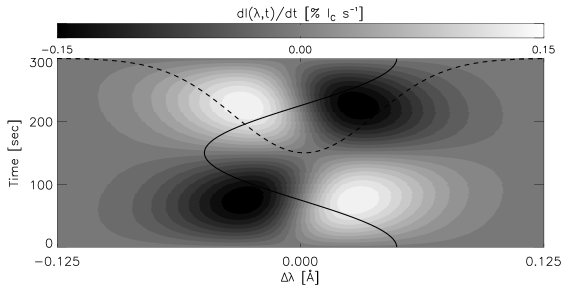
Figure 3: Contour plot of the amount of cross talk per unit time (in units of % of the continuum intensity) induced into the polarization profiles from the total intensity as a consequence of the solar p modes (see Equation (19) and text for details). Horizontal axis indicates relative position with respect to the central laboratory wavelength. Vertical axis indicates time in which the measurement is taken within one oscillatory period of 300 seconds. Relative amplitudes are indicated by the gray scale bar at the top of the plot. For visualization purposes, a magnified example of the Fe I 6173 Å  spectral line has been over plotted in dashed lines. Temporal evolution of the p-mode velocity $\xi(t)$ (see Equation (18)) is indicated by the solid lines.

Besides this analytical estimate, we have carried out a more detailed analysis by taking into account all possible effects and a realistic p-mode function $\xi(t)$ (Figure 2 top panel). For this analysis we used 20 000 Stokes profiles $\widetilde{{\rm{\bf{I}}}}^{\rm obs}(\lambda_{j},t_{n})$ that were converted into $\widetilde{{\rm{\bf{I}}}}^{\rm obs}(\lambda_{i})$ according to Section 2. Polarization levels, defined as ${\rm max}|V|$ and ${\rm max}|\sqrt{Q^{2}+U^{2}}|$ in units of percentage of the continuum intensity, are compared before and after. Results are displayed in Figure 4. The horizontal axis refers to the polarization levels from the original profiles: $\widetilde{{\rm{\bf{I}}}}^{\rm obs}(\lambda_{i},t_{n})$ as in Equation (3). The vertical axis represents the polarization levels of the profiles once the effects of the solar p modes have been taken into account: $\widetilde{{\rm{\bf{I}}}}^{\rm obs}(\lambda_{i})$ as in Equation (4). Random initial times $t_{0}$ are used for sampling the function $\xi(t)$ (see Figure 2; top panel). The experiment is repeated for all modulation schemes (see Section 2). As can be seen, modulation scheme A introduces a large amount of cross talk into the circular polarization while keeping the cross talk into the linear polarization within reasonable limits.

As already mentioned, this effect is ultimately related to the modulation matrix $\mathcal{M}$. In scheme A, $\mathcal{O}_{1}(\lambda_{i},t_{0})=I-0.81Q+0.588V$ it is the first measurement. The next one corresponds to $\mathcal{O}_{2}(\lambda_{i},t_{0}+\Delta t)=I-0.81Q+0.588V$ and therefore, Stokes $Q(\lambda_{i})$ can be constructed with measurements done only $\Delta t=$ four seconds apart from each other, thereby minimizing the amount of cross talk from Stokes $I$. However, Stokes $V$ is built out of a combination of measurements taken far away in time. For example: $\mathcal{O}_{1}(\lambda_{i},t_{0})=I+0.81Q+0.588V$ is measured at $t_{0}$, but $\mathcal{O}_{3}(\lambda_{i},t_{0}+[2M+1]\Delta t)=I+0.81U-0.588V$ is recorded 44 seconds later (see Table I). During this time the solar p modes might introduce large levels of cross talk from Stokes $I$ into Stokes $V$. This also explains why scheme B introduces large cross talk into the linear polarization while leaving the circular polarization almost unchanged. As expected, Modulation scheme C performs well both in linear and circular polarization. The obvious drawback to Scheme C is that it takes longer to scan across the line: $6M\Delta t$ seconds as compared to $4M\Delta t$ seconds from schemes A and B. Thus, scheme C minimizes the short time scale p-mode effect but maximizes the long time scale p-mode effect. In order to study which effect introduces larger errors when retrieving the magnetic field vector, inversion of simulated profiles are required.

Figure 4: Polarization cross talk induced by the short time solar p-mode effect for the three polarization modulations under consideration: scheme A (top panels), scheme B (middle panels) and scheme C (bottom panels). Horizontal axis refer to the original polarization levels (in percentage of the continuum intensity units). Vertical axis indicate the polarization levels after the p-mode effect has been taken into account. Left panels are for the linear polarization: $\sqrt{Q^{2}+U^{2}}$. Right panels for the circular polarization: $V$. See text for further details.

4 Inversion strategy

4.1 OBSERVED PROFILES

Prior to the inversion, we must obtain a sufficiently large number of observed Stokes profiles whose atmospheric parameters are known. To this end we have built up a data base of atmospheric parameters with more than 20 000 atmospheres. Each of those is represented by a set of parameters ${\rm{\bf{X}}}_{\rm r}=[{\rm B},\gamma,\psi,{\rm v}^{\rm LOS},{\rm S},{\rm\dot{S}},\alpha]$. Each ${\rm{\bf{X}}}_{\rm r}$ is used to produced a synthetic (that simulates observed ones) Stokes vector: ${\rm{\bf{I}}}^{\rm obs}(\lambda_{j})$ sampled in 300 wavelength positions to approximate a continuos function (Equation (3)). This is done according to Equation (10). Note that ${\rm{\bf{X}}}_{\rm r}$ is used to synthesize the magnetic atmosphere: ${\rm{\bf{I}}}^{\rm mg}(\lambda_{j})$. To this profile we add a non-magnetic contribution ${\rm{\bf{I}}}^{\rm nm}(\lambda_{j})$ whose shape is known.

A random time ($t_{0}$) and a modulation matrix ($\mathcal{M}$) must also be chosen. According to this and Equation (3) the HMI filter profiles $\mathcal{G}_{i}$ are applied and $\widetilde{{\rm{\bf{I}}}}^{\rm obs}(\lambda_{i},t_{0})$ is obtained at wavelength position $\lambda_{i}$. A linear combination of the components of $\widetilde{{\rm{\bf{I}}}}^{\rm obs}(\lambda_{i},t_{0})$ is produced through Equation (1): $\mathcal{O}_{p}(\lambda_{i},t_{0})$. The next linear combination $\mathcal{O}_{p+1}(\lambda_{i},t_{0}+\Delta t)$ at the same wavelength position is obtained out of $\widetilde{{\rm{\bf{I}}}}^{\rm obs}(\lambda_{i},t_{0}+\Delta t)$, where these profiles have been shifted in wavelength to account for the variation over that time interval $\Delta t$ of the function $\xi(t)$ (see Equation (12) and Figure 2). Note that the only velocity that changes in time is the p-mode velocity $\xi(t)$. In Equation (12) ${\rm v}^{\rm LOS}_{\rm plasma}$ corresponds to ${\rm v}^{\rm LOS}$ from ${\rm{\bf{X}}}_{\rm r}$ and does not change during the observing time. Unless otherwise specified, photon noise is also added to each $\mathcal{O}_{p}(\lambda_{i},t_{0})$ according to Section 3.1.

In Figure 2, the rms amplitude of the p-mode velocity is about 250 m s^-1. This was obtained from a two-hour MDI temporal series in the quiet Sun using the high resolution field of view. For magnetized regions the amplitude of the solar p modes is known to decrease, however. To this end, the rms value of the $\xi(t)$ function in Figure 2 is scaled with the magnetic field $\rm B$ from ${\rm{\bf{X}}}_{\rm r}$ according to (see Norton, 2000):

$$\xi_{rms}(t) = \left\{\begin{array}[]{rr}250-0.155\times{\rm B}&\;\;\;\;{\rm if}\;\;\;{\rm B}\leq 1000~{}G\\ 128-0.033\times{\rm B}&\;\;\;\;{\rm if}\;\;\;{\rm B}>1000~{}G\\ \end{array}\right\}\;\;\;{\rm[m\;s^{-1}]}$$ (22)

Once all needed $\mathcal{O}_{p}(\lambda_{i})$, with $p=1,...,P$, are known at wavelength position $\lambda_{i}$, the final observed vector $\widetilde{{\rm{\bf{I}}}}^{\rm obs}(\lambda_{i})$ is obtaining by demodulating as in Equations (4) - (5). An example of ${\rm{\bf{I}}}^{\rm obs}(\lambda_{j},t_{0})$ is given in Figure 5 (top four panels; dashed line). In circles we also plot the observed profiles, $\widetilde{{\rm{\bf{I}}}}^{\rm obs}(\lambda_{i},t_{0})$, after the filters $\mathcal{G}$ have been applied. In the lower four panels in Figure 5, $\widetilde{{\rm{\bf{I}}}}^{\rm obs}(\lambda_{i},t_{0})$ is plotted again. Here we added $\widetilde{{\rm{\bf{I}}}}^{\rm obs}(\lambda_{i})$, which are the observed profiles after the effects of the solar p modes have been introduced. Modulation schemes A (dotted lines), B (dashed lines) and C (dashed-dotted lines) have been used. In the three cases, the same $t_{0}$ was employed. This plot also shows how the solar p modes affect the circular polarization more when scheme A is used, and have a stronger effect in the linear polarization profiles when scheme B is employed.

Figure 5: Top 4 panels: Normalized original Stokes profiles ${\rm{\bf{I}}}^{\rm obs}(\lambda_{j})$ evaluated in 300 wavelength points (dashed lines). Profiles $\widetilde{{\rm{\bf{I}}}}^{\rm obs}(\lambda_{i})$ after convolution with HMI filter profiles (Equation (3); circles). Bottom 4 panels: circles as in the top panels. Dotted, dashed and dashed-dotted lines corresponds to the profiles observed by HMI, $\widetilde{{\rm{\bf{I}}}}^{\rm obs}(\lambda_{i})$ (see Equation (4)), when modulation schemes A, B, and C, respectively, are used. No photon noise has been considered here.

4.2 INVERSION DETAILS

Once HMI observed profiles $\widetilde{{\rm{\bf{I}}}}^{\rm obs}(\lambda_{i})$ are available, the next step is to try to recover the photospheric parameters ${\rm{\bf{X}}}_{\rm r}$ that produced them. The underlying idea of this inverse process consists in producing a initial synthetic Stokes profiles $\widetilde{{\rm{\bf{I}}}}^{\rm syn}(\lambda_{i})$ out of an initial set of photospheric parameters ${\rm{\bf{X}}}_{\rm 0}$ by solving the analytical Milne-Eddington solutions to the RTE. The synthetic profiles are compared to the observed ones and ${\rm{\bf{X}}}_{\rm 0}$ is modified until the observations are matched. The way this works is by building a $\chi^{2}$ or merit function as follows:

$$\chi^{2} = \frac{1}{L}\sum_{k=1}^{4}\sum_{i=1}^{M}\left[\frac{\widetilde{I}_{k}^{\rm obs}(\lambda_{i})-I_{k}^{\rm syn}({\rm{\bf{X}}},\lambda_{i})}{\sigma_{ik}}\right]^{2}w_{k}^{2}$$ (23)

where $L$ is the total number of free parameters (i.e.: seven parameters defining ${\rm{\bf{X}}}_{\rm r}$), and the indexes k and i run for the four components of the Stokes vector and for all wavelengths in which the spectral line is sampled $M=5$. $\sigma_{ik}$ is a measure of the errors in the observations (i.e.: photon noise) and $w_{k}$ is a factor used to ensure that the contribution on the derivatives of $\chi^{2}$ with respect to the free parameters is not dominated by derivatives with respect to Stokes $I$. To this end, we adopt:

$$w_{k}^{2} = \frac{1}{max\{[I_{k}(\lambda)^{2}]\}}$$ (24)

Once $\chi^{2}$ is built, we numerically calculate the derivatives of the merit function with respect to the free parameters which are then used by a non-linear Levenberg-Marquardt least squares fitting algorithm (Press et al. 1986) together with a modified Singular Value Decomposition method (Ruiz Cobo and Del Toro Iniesta, 1992). The algorithm returns the vector of free parameters X${}_{\rm f}=[\rm B_{f},\gamma_{f},\psi_{f},V^{LOS}_{f},S_{f},\dot{S}_{f},\alpha_{f}]$ that minimizes $\chi^{2}$ and defines the actual (i.e.: real) solar atmosphere: ${\rm{\bf{X}}}_{\rm r}={\rm{\bf{X}}}_{f}$.

As pointed out, the inversion requires the use of an initial guess model ${\rm{\bf{X}}}_{0}$. In order to make the simulation as realistic as possible, we choose to fix the initial set of parameters (see Table V) that will be kept for all inverted profiles. In that way we assume no previous knowledge of the real ${\rm{\bf{X}}}_{\rm r}$. Besides the initial set of parameters (${\rm{\bf{X}}}_{0}$) we run a number of extra inversions of each Stokes vector but using randomly generated ${\rm{\bf{X}}}$’s, and only the one that retrieves the smallest $\chi^{2}$ is kept.

It is important to mention that our set of free parameters (see Table V) does not include the Doppler width, line-to-continuum opacity ratio and damping (parameters also used by the Milne-Eddington model). This strategy has been adopted to mimic the number of free parameters of a full inversion method (see for instance Ruiz Cobo and Del Toro Iniesta, 1992) where the neglected parameters are determined through the temperature stratification $T(\tau)$.

Table V: Initial set of physical parameters X₀ used in the inversion. We only assume a previous knowledge in the magnetic field inclination, where $\gamma<90^{\circ}$ or $>90^{\circ}$ is chosen depending on the sign in Stokes $V$ lobes. Note that the Doppler width, opacity ratio and damping parameters are not considered as free parameters (see text for details).

Physical Parameter	Symbol	Value
Magnetic field strength	B	1000 Gauss
Magnetic field inclination	$\gamma$	60 - 120∘
Magnetic field azimuth	$\psi$	30∘
Line-of-sight velocity	vLOS	2.5 km s-1
Source Function	S	0.3
Source Function Gradient	$\rm\dot{S}$	0.45
Filling Factor	$\alpha$	0.5

5 Effect of Polarization Modulation

In this section we will study which polarization scheme allows for a better recovery of the physical photospheric parameters ${\rm{\bf{X}}}_{\rm r}$ and in particular of the magnetic field vector. To this end, three simulations (see Section 4 for details) were carried out using a different modulation matrix $\mathcal{M}$ (see Equations (6) – (8)). Each of them includes the inversion of 20 000 individual profiles. Those profiles were produced using a set of photospheric parameters (${\rm{\bf{X}}}_{\rm r}$), and a initial random time $t_{0}$ to take into account the solar p modes (as in Figure 2; top panel). The p-mode function $\xi(t)$ was scaled according to Equation (20). At this point, photon noise was not taken into account. The inversion of each profile returns a set of inverted atmospheric parameters (${\rm{\bf{X}}}_{\rm f}$) that can be compared to the real one (${\rm{\bf{X}}}_{\rm r}$). This allows us to study the error in the retrieval of those parameters.

Figure 6 displays the errors in the retrieval of magnetic field strength (top left panel), magnetic field inclination (top right panel), magnetic field azimuth (bottom right panel) and line-of-sight velocity (bottom left panel). The errors are presented as a function of the physical parameter itself. This measure is taken by sorting the differences between the real and inverted values in increasing order and picking the value that leaves 68 % of the 20 000 inverted profiles below it. This provides a robust measure of the standard deviation in the inferred parameters and will be used hereafter as error.

In spite of having the longest observing sequence ($30\Delta t$ seconds), scheme C minimizes the errors in the retrieved parameters. This indicates that the short term p-mode effect is more important than the long one (see Section 3.2). In this sense, scheme C ensures that the induced cross talk is minimized since orthogonal observations are done with only $\hat{t}=\Delta t=$ four seconds delay (see Equations (13) – (14)).

Figure 6: Errors in the retrieval of the different physical parameters as a function of the parameter itself. Top left panel: magnetic field strength; Top right panel: magnetic field inclination; Bottom left panel: line-of-sight velocity; Bottom left panel: magnetic field azimuth. Different line styles correspond to: modulation scheme A (solid; Equation (6)), scheme B (dotted; Equation (7)), scheme C (dashed; Equation (8)).

• Magnetic field strength: scheme A does a better job that scheme B. The main reason for this is to be found in the generally smaller amplitudes of Stokes $Q$ and $U$ with respect to Stokes $V$. The same amount of cross talk will alter more significantly the linear polarization than the circular, thereby affecting in a more severe manner the recovered values for $B_{\perp}$ in scheme B than the retrieved $B_{\parallel}$ in scheme A. Note that all schemes show an increase in the errors when the field strength grows above 1500 Gauss. This is related to saturation effects: for larger fields, the Zeeman splitting is large enough to shift the spectral line out of the scanned region, resulting in a loss of information. For small field strengths the high increase in the errors, in particular for schemes A and B, is mainly due to the larger amplitude of the p modes (Equation (20)).

• Magnetic field azimuth: as expected, scheme A retrieves smaller errors than scheme B. The reason is that the field azimuth angle depends on the ratio $\sim Q/U$ (Jefferies and Mickey, 1991). Since scheme A minimizes the p-mode cross talk into the linear polarization (see Figure 4), it retrieves more accurate azimuthal angles.

• Magnetic field inclination: scheme B gives slightly superior performance as compared to scheme A. This has no trivial explanation, since this parameter depends on both linear and circular polarization. In addition, all three modulation schemes display this kind of behavior in $\sigma_{\gamma}$ as a function of $\gamma$. The error increases towards $\gamma\rightarrow 0^{\circ},180^{\circ}$, while it is minimum at $\gamma\sim 90^{\circ}$.

Another interesting comparison can be made by plotting the error as a function of the filling factor of the magnetic component ($\alpha$). This is done in Figure 7. Errors increase with decreasing $\alpha$ for all physical parameters and for all modulation schemes. The reason in this case is trivial. The closer $\alpha$ is to 0, the less amount of total observed light comes from the magnetic atmosphere ${\rm{\bf{I}}}^{\rm mg}$ (see Equations (10) – (11)), therefore becoming increasingly more difficult to infer its properties. Hereafter we will focus in the modulation schemes A and C, since scheme B can be ruled out due to the larger errors that introduces.

Figure 7: Same as in Figure 6 but as a function of the filling factor of the magnetic component ($\alpha$).

6 Effect of the Photon Noise

The simulations in Section 5 did not include photon noise. Therefore, the next step in our analysis is to consider the simultaneous effect of the solar p modes and the photon noise. To this end we have carried out two new simulations where HMI profiles were obtained using modulation schemes A and C and taking into account the expected photon noise (see Section 3.1). Errors as a function of the filling factor of the magnetic component ($\alpha$) are presented in Figure 8 in thick lines (solid for scheme A and dashed for scheme C). For comparison purposes we plot also the results from schemes A and C from Section 5 (where only solar p modes were considered) in thin lines. By comparing thin and thick lines in Figure 8 one can see that errors introduced by the photon noise are dominant over those induced by the solar p modes.

An interesting effect appears after introducing the photon noise. As already mentioned in Section 5, the errors (when only p modes are considered) decrease with decreasing filling factor. This is generally also the case when p modes and photon noise are considered simultaneously. However, for large filling factors, $\alpha\rightarrow 1$, this effect is less pronounced. For some physical parameters, like the field strength (Figure 8; top left panel) errors even tend to slightly increase. This might be related to the fact that in our simulations, those points of the database with large filling factors are intended to represent umbral points. The reduced light level in those regions translates into a smaller signal-to-noise in the observed profiles, thereby increasing the errors in the retrieval of the magnetic properties.

Figure 8: Errors in the retrieved physical parameters as a function of the filling factor of the non-magnetic component. Thin lines correspond to the results when only p modes are considered (same as in Figure 7). Thick lines corresponds to results when solar p modes and photon noise (pn) are taken into account. Schemes A and C are indicated in solid and dashed lines, respectively.

7 Temporal Averages

In Section 3 we pointed out that at a given wavelength the crosstalk induced by the solar p modes changes sign as the oscillation goes from the increasing velocity regime to the decreasing part of the wave (see Figure 3). By averaging in time the observed signal, the p-mode crosstalk should be minimized. This effect is shown in Figure 9 where we plot in circles the original profiles as if no p modes existed: $\widetilde{{\rm{\bf{I}}}}^{\rm obs}(\lambda_{i})$. Overploted in dashed lines are Stokes $V$ observed during consecutive time intervals: $[t_{0},t_{0}+4PM]$, $[t_{0}+4PM,t_{0}+8PM]$, etc. They are computed considering the p modes. These dashed profiles recorded during $PM\Delta t$ seconds will be referred to as building block profiles. Since they are consecutive in time, the time-dependent behavior of the solar oscillation (see Figure 2; top panel) is sampled, each of them contributing differently to the induced crosstalk. When all building blocks are averaged, the resulting profile (solid lines in Figure 9) closely resembles that without p-mode contribution (circles).

Figure 9 is obtained from a total averaging time of 480 seconds (roughly 1.5 oscillatory periods). Note that, as imposed by Equation (6) and Equation (8), for modulation scheme A (left panel) the individual observations (dashed lines) are much more affected by the solar p modes than for scheme C (right panel). This does nothing but to stress the results from Figure 4. Interestingly, the averaged Stokes $V$ (solid line) are in both cases very similar. The reason for this is that during 480 seconds, scheme A is able to observe Stokes $V$ as many as six times: $P=4\rightarrow\widetilde{t}=80$ seconds. Scheme C is able to record Stokes $V$ only four times: $P=6\rightarrow\widetilde{t}=120$ seconds. This allows scheme A to provide a better sampling of the solar p-mode oscillations, thus reducing more efficiently the induced crosstalk.

Therefore, it is important to quantify how results compare when using different averaging times. In particular, whether scheme A becomes at some point more reliable than scheme C. To this end we have carried out several simulations using different averaging times with modulation schemes A and C. In these simulations photon noise was added to the building block profiles according to Section 3.1. The averaged profiles obviously present a larger signal-to-noise. Some important properties of the simulations are presented in Table VI.

Table VI: Main properties of the simulations carried out in Section 6. First column indicates the modulation scheme used. The asterisk indicates a simulation done with the minimum time required to sample the full Stokes vector for that particular scheme: building block profiles. Second column refers to the amount of total time used to average profiles. Note that it is always an integer multiple of the building block. Third column is the total number of times that the full Stokes vector ${\rm{\bf{I}}}$ is sampled during the time indicated in the second column. Last column shows the noise level ($\sigma_{i}$) in the averaged polarization profiles. This is indicated in units of noise level in the building block observation using scheme C.

Scheme	Averaging time [sec]	# Stokes ${\rm{\bf{I}}}$	$\sigma_{i}$
A	880	10	0.369
A	560	7	0.462
A	240	3	0.707
A∗	80	1	1.22
C	840	7	0.377
C	600	5	0.447
C	240	2	0.707
C∗	120	1	1

Figure 10 shows the errors in the physical parameters as a function of the time used to average. Note that the temporal evolution of solar structures over the averaging time is neglected (except for the solar p modes). In this sense the retrieved physical parameters should be considered as an average of the physical conditions present in the solar atmosphere during the time the data is acquired. Results are presented considering three different solar structures: sunspots, plages and network regions. Those definitions are given according to the filling factor of the magnetic atmosphere. Sunspots: $\alpha\in[0.7,1]$, Plage: $\alpha\in[0.4,0.6]$, Network: $\alpha\in[0.1,0.3]$. With the exception of the velocity, scheme A (thin lines) becomes more reliable than scheme C (thick) using an averaging time as short as 240 seconds. For large averaging times, both observing schemes become almost identical. The HMI scientific goal is to provide the full magnetic field vector with a cadence of ten minutes. At this level the errors for sunspot regions could be as little as $\sigma_{B}\sim 4$ Gauss, $\sigma_{\gamma}\sim 0.2^{\circ}$, $\sigma_{\psi}\sim 0.2^{\circ}$ and $\sigma_{v}\sim 20$ m s^-1 (see Tables VII and VIII for details).

Figure 9: Left panel: example of Stokes $V$ profiles as observed by HMI neglecting the effect of the solar p modes (circles). Dashed lines represent individual observations in consecutive time intervals where solar p modes were accounted for using scheme A. Each observation requires $5P\Delta t$ seconds. The average of all of these observations is represented by the solid line. Right panel: same but using scheme C. Photon noise was not included in these examples.

Figure 10: Errors in the determination of the different physical parameters as a function of the averaging time. Thin lines indicate results for modulation scheme A whereas thick ones are for scheme C. Different line styles correspond to different observed solar regions: sunspots (solid), plage (dotted) and network regions (dashed).

Region	$\sigma_{B}$	$\sigma_{\gamma}$	$\sigma_{\psi}$	$\sigma_{v}$
	[Gauss]	[deg]	[deg]	[m s-1]
Sunspot	4 - 5	0.2	0.2	20
Plage	10	1	1	30
Network	40 - 50	2 - 3	5 - 7	60 - 90

Table VII: Approximate errors in the determination of the properties (magnetic field vector, velocity) of the magnetic component. This corresponds to a ten minute temporally averaged data product.

Region	$\sigma_{B}$	$\sigma_{\gamma}$	$\sigma_{\psi}$	$\sigma_{v}$
	[Gauss]	[deg]	[deg]	[m s-1]
Sunspot	30	1	1	40
Plage	80 - 100	4	6 - 8	100 - 200
Network	400 - 700	30	30 - 50	$>$ 1000

Table VIII: Approximate errors in the determination of the properties (magnetic field vector, velocity) of the magnetic component. This corresponds to a 120 second data product (building block profiles) using Mod C.

8 Conclusions

The HMI instrument intends to provide accurate and continuous full-disk measurements of the solar magnetic field vector in the photosphere. We have identified and carefully studied the main sources of errors in HMI: limited spectral resolution, solar p modes (that affect our data as a consequence of the non-simultaneity in the polarization measurements) and photon noise. The most critical source of error turns out to be the photon noise. Increasing the signal-to-noise ratio of the observations is achieved with longer integration times. This is not trivial. Increasing the exposure time per measurement may lead to saturation effects as we reach the limits of the CCD’s linear behavior. The only possibility left is to combine several measurements. We find that averaging data over ten minutes increases the signal-to-noise by a factor of two to three (see Table VI) plus effectively removes the effect of the solar p modes. This leads to very precise determinations of the time-averaged magnetic field vector, with an accuracy better than five Gauss in field strength and 0.2 degrees in inclination and azimuth.

A faster and better correction for the p modes can be achieved in different ways. On the one hand, the observations can be averaged over time using more sophisticated methods. In Section 7 a simple (unweighted) average was used. More sophisticated ways (e.g.: using appropriate weights) would lead to a faster smearing of the solar p modes. On the other hand, it is possible to interpolate the data so that we combine polarization measurements taken at the same time (see Equation (14)). This might correct the effects of the solar p modes even without time averaging. A last possibility would be to apply a subsonic filter to the raw (i.e.: monochormatic and not demodulated) data (Rutten, Wijn, and Sütterlin, 2004). Although these possibilities are worth investigating, they will not significantly change our results since the main source of errors is the photon noise.

A critical point we have not mentioned concerns the contribution of the non-magnetic atmosphere ${\rm{\bf{I}}}^{\rm nm}$ (see Equation (10)). In all our simulations we have considered ${\rm{\bf{I}}}^{\rm nm}$ as known (with the exception of the filling factor $\alpha$). This is a best case scenario. In reality, the ${\rm{\bf{I}}}^{\rm nm}$ contribution can arise because of scattered light from the optical elements of the instrument, or due to the presence of a real non-magnetic atmospheric component within the resolution element of the observations.

In the first case (instrumental scattered light), it might be possible to characterize ${\rm{\bf{I}}}^{\rm nm}$ with laboratory tests. In the second case, its origin would be solar, and therefore we should have considered new free parameters in our inversion to describe ${\rm{\bf{I}}}^{\rm nm}$, such as: ${\rm v^{\rm LOS}_{\rm nm}},{\rm S_{\rm nm}},{\rm\dot{S}_{\rm nm}}$. We have neglected this in order to keep the number of free parameters (listed in Table IV) within reasonable limits and below the number of data points (20). A necessary extension of this work should address this point carefully by both (a) including the new free parameters and, (b) by using a different ${\rm{\bf{I}}}^{\rm nm}$ in the synthesis and the inversion so that we can quantify the errors introduced by a poorly known ${\rm{\bf{I}}}^{\rm nm}$. Obviously the larger $\alpha$, the smaller these errors will be. Therefore, for sunspot regions (Figure 10 and Tables VII and VIII) the results presented in this work should be robust.

Another very important issue concerns the speed of the inversion process (see Section 4). The employed method is a traditional non-linear least-squares fitting algorithm. This method will not ultimately be used for the inversion of HMI data. Our simulations with the analysis of 20 000 profiles took an average of 24 hours to complete. HMI requires the processing of millions of profiles per minute. Even those methods, considered to be fast, such as Principal Component Analysis (Rees et al., 2000) or Artificial Neural Networks (Socas-Navarro, 2003), will be challenged by HMI requirements. This will be the subject of a future investigation.

References

• Cabrera Solana, D., Bellot Rubio, L.R, and del Toro Iniesta, J.C.: 2005, Astron. Astrophys. , 439, 687.

• Graham, J.D., López Ariste, A., Socas-Navarro, H., and Tomczyk, S.: 2002, Solar Phys., 208, 211.

• Graham, J.D., Norton, A.A, Ulrich, R.K. et al.: 2003, HMI-TN-03-002. http://hmi.stanford.edu/doc/Tech_Notes/TechNoteIndex.html

• Jefferies, J.T. and Mickey, D.L.: 1991, Astrophys. J., 372, 694.

• Landi Degl’Innocenti, E.: 1991, in F. Sánchez, M. Collados and M. Vázques (eds.), Solar Observations: Techniques and Interpretation. First Canary Islands Winter School of Astrophysics.. Cambridge University Press.

• Norton, A.A.: 2000, Ph.D Thesis, Univ. California Los Angeles.

• Norton, A.A., Pietarila Graham, J., Ulrich, J.K., Schou, J., Tomczyk, S., Liu, Y., Lites, B., Lopez Ariste, A., Bush, R., Socas Navarro, H., Scherrer, P., 2006, Solar Phys., in press.

• Press, W.H., Flannery, B.P., Teukolsky, S.A., and Vetterling, W.T.: 1986, Numerical Recipes, Cambridge University Press.

• Rees, D.E., López Ariste A., Thatcher, J., and Semel, M.: 2000, Astron. Astrophys., 355, 759.

• Ruiz Cobo, B. and del Toro Iniesta, J.C.: 1992, Astrophys. J., 398, 375.

• Rutten, R.J., de Wijn, A.G. & Sütterlin, P.: 2004, Astron. Astrophys., 416, 333.

• Scherrer, P.H., Bogart, R.S., Bush, R.I. et al.: 1995, Solar Phys., 162, 129.

• Socas-Navarro, H.: 2003, Neural Networks, 16, 355.

• del Toro Iniesta, J.C. 2003, Introduction to Spectropolarimetry, Cambridge University Press.

• del Toro Iniesta, J.C. and Collados, M.: 2000, Applied Optics, 39, 1637.