A study of Jupiter’s aurorae with XMM-Newton

Abstract

We present a detailed analysis of Jupiter’s X-ray (0.2$-$10 keV) auroral emissions as observed over two XMM-Newton revolutions in Nov. 2003 and compare it with that of an earlier observation in Apr. 2003. We discover the existence of an electron bremsstrahlung component in the aurorae, which accounts for essentially all the X-ray flux above 2 keV: its presence had been predicted but never detected for lack of sensitivity of previous X-ray missions. This bremsstrahlung component varied significantly in strength and spectral shape over the 3.5 days covered by the Nov. 2003 observation, displaying substantial hardening of the spectrum with increasing flux. This variability may be linked to the strong solar activity taking place at the time, and may be induced by changes in the acceleration mechanisms inside Jupiter’s magnetosphere. As in Apr. 2003, the auroral spectra below 2 keV are best fitted by a superposition of line emission most likely originating from ion charge exchange, with OVII playing the dominant role. We still cannot resolve conclusively the ion species responsible for the lowest energy lines (around 0.3 keV), so the question of the origin of the ions (magnetospheric or solar wind) is still open. It is conceivable that both scenarios play a role in what is certainly a very complex planetary structure.

High resolution spectra of the whole planet obtained with the XMM-Newton Reflection Grating Spectrometer in the range 0.5$-$1 keV clearly separate emission lines (mostly of iron) originating at low latitudes on Jupiter from the auroral lines due to oxygen. These are shown to possess very broad wings which imply velocities of $\sim$5000 km s^-1. Such speeds are consistent with the energies at which precipitating and charge exchanging oxygen ions are expected to be accelerated in Jupiter’s magnetosphere. Overall we find good agreement between our measurements and the predictions of recently developed models of Jupiter’s auroral processes.

1 Introduction

The current generation of X-ray observatories, with their unprecedented spatial resolution (Chandra) and sensitivity (XMM-Newton), coupled to moderate (CCD) to high (gratings) spectral resolution, have made it feasible for the first time to study solar system objects in detail. Jupiter has a particularly complex magnetospheric environment, which is governed by its fast rotation and by the presence of Io and its dense plasma torus. Not surprisingly the giant planet became a target of observations since the earliest attempts at X-ray studies of the solar system: Jupiter was first detected in X-rays with the Einstein observatory (Metzger et al. [1983]), and was later studied with ROSAT (e.g. Waite et al. [1994]).

By analogy with the Earth’s aurorae, Jupiter’s X-ray emission was expected to be produced via bremsstrahlung radiation by energetic electrons precipitating from the magnetosphere and scattered by nuclei in the planet’s upper atmosphere. However, the observed X-ray spectrum was softer (0.2$-$3 keV) and the observed fluxes higher than expected for a bremsstrahlung origin, implying unrealistically high electron input power with respect to that required to produce the UV aurora (Metzger et al. [1983]). The alternative is K shell line emission from ions, mostly of oxygen, which are stripped of electrons while precipitating, and then charge exchange: the ions are left in an excited state from which they decay back to the ground state with line emission (see Bhardwaj et al. [2006b] for a recent review of solar system X-ray observations and emission mechanisms). The origin of the precipitating ions was naturally postulated to be in Jupiter’s inner magnetosphere, where an abundance of sulphur and oxygen ions, associated with Io and its plasma torus, could be found (Metzger et al. [1983]). The latter alternative was given support by ROSAT soft X-ray (0.1$-$2.0 keV) observations which produced a spectrum much more consistent with recombination line emission than with bremsstrahlung (Waite et al. [1994], Cravens et al. [1995]).

To test the bremsstrahlung hypothesis, Waite ([1991]) and Singhal et al. ([1992]) carried out model calculations for the energy deposition by primary electrons with a Maxwellian energy distribution precipitating in Jupiter’s upper atmosphere and producing secondary electrons by ionisation: both these works indeed confirmed that the expected bremsstrahlung flux is smaller by up to 3 orders of magnitude compared with the observed $<$2 keV X-ray flux. Singhal et al. concluded that only high-energy ($>$2 keV) X-ray observations could resolve the question of the identity and energy of the particles involved in producing the full spectrum of auroral emissions on Jupiter. The XMM-Newton observations reported in the present paper address precisely this issue.

Chandra observations have given us the sharpest view of Jupiter’s X-ray emission, but have also raised serious questions: HRC-I observations in Dec. 2000 and Feb. 2003 clearly resolve two bright, high-latitude sources associated with the aurorae, as well as diffuse low-latitude emission from the planet’s disk (Gladstone et al. [2002], Elsner et al. [2005], Bhardwaj et al. [2006a]). However, the Northern X-ray hot spot is found to be magnetically mapped to distances in excess of 30 Jovian radii from the planet, rather than to the inner magnetosphere and the Io plasma torus, as originally speculated (see Bhardwaj and Gladstone [2000] for a review). Since in the outer magnetosphere ion fluxes are insufficient to explain the observed X-ray emission, another ion source (likely the solar wind) may be contributing; in any case, an acceleration mechanism needs to be present in order to boost the flux of energetic ions: potentials of $\sim$200 kV and at least 8 MV are needed in case of a solar wind and magnetospheric origin respectively (Cravens et al. [2003]). Strong 45 min quasi-periodic X-ray oscillations were also discovered by Chandra in the North auroral spot in Dec. 2000. No correlated periodicity was seen at the time in Cassini upstream solar wind data, nor in Galileo and Cassini energetic particle and plasma wave measurements (Gladstone et al. [2002]).

The Chandra 2003 ACIS-S observations (Elsner et al. [2005]) show that the auroral X-ray spectrum is made up of line emission consistent with high charge states of oxygen, with a dominant fraction of fully stripped ions. Line emission at lower energies could be from sulphur (0.31$-$0.35 keV) and/or carbon (0.35$-$0.37 keV): were it from carbon, it would suggest a solar wind origin. The high charge states imply that the ions must have undergone acceleration, independently from their origin, magnetospheric or solar wind. Rather than periodic oscillations, chaotic variability of the auroral X-ray emission was observed, with power peaks in the 20$-$70 min range; similar power spectra were obtained from the time history of Ulysses radio data taken at 2.8 AU from Jupiter at the time of the Chandra observations (Elsner et al. [2005]). A promising mechanism which could explain the change in character of the variability, from organised to chaotic, is pulsed reconnection at the day-side magnetopause between magnetospheric and magnetosheath field lines, as suggested by Bunce et al. ([2004]). This process, occurring at the Jovian cusps, would work equally well for ions of magnetospheric origin as for ions from the solar wind.

With its unparalleled photon collecting area up to $\sim$10 keV XMM-Newton has the potential of providing high signal-to-noise spectra with which to try and resolve some of the un-answered issues surrounding Jupiter and its environment. XMM-Newton has observed Jupiter twice: in Apr. 2003 (110 ks; Branduardi-Raymont et al. [2004], BR1 hereafter), and in Nov. 2003 (245 ks).

The Apr. 2003 XMM-Newton European Photon Imaging Camera (EPIC) soft X-ray spectra of Jupiter’s auroral spots can be modelled with a combination of emission lines, including most prominently those of highly ionised oxygen; however, unlike the Chandra ACIS-S spectra where the emission appears to be mostly from OVIII (0.65 keV, or 19.0 Å), the EPIC data require a dominant contribution from OVII He-like transitions (0.57 keV, or $\sim$22 Å). A 2.8$\sigma$ enhancement in the Reflection Grating Spectrometer (RGS) spectrum at 21$-$22 Å is consistent with the OVII identification. At lower energies the EPIC best fit model includes an emission line centred at 0.36 $\pm$ 0.02 keV for the North aurora and at 0.33${}^{\rm+0.02}_{\rm-0.03}$ keV for the South, which would suggest a CVI Ly$\alpha$ transition (0.37 keV) rather than emission from SXI$-$SXIII (0.32$-$0.35 keV). While this would support a solar wind origin, BR1 point out that the rather poor statistical quality of the data make line discrimination uncertain.

The X-ray spectrum of Jupiter’s low latitude disk regions is different, and matches that of solar X-rays scattered in the planet’s upper atmosphere (BR1; see also Maurellis et al. [2000], Cravens et al. [2006]). A temporal study of Jupiter’s low latitude disk emission during the Nov. 2003 XMM-Newton observation and of its relationship to the solar X-ray flux is presented in Bhardwaj et al. ([2005]), while a spectral analysis of the disk emission is given in Branduardi-Raymont et al. ([2006]).

Here we present a detailed study of Jupiter’s auroral emissions from the analysis of the Nov. 2003 XMM-Newton observation, which we compare with that of Apr. 2003, and with the Chandra data, as appropriate: Sect. 2 of this paper covers the analysis of the temporal behaviour; in Sect. 3 we present EPIC images in selected spectral bands; our modelling of the EPIC auroral spectra is described in Sect. 4, and the analysis of the RGS high resolution spectrum of the planet is reported in Sect. 5. Discussion and conclusions follow in Sects 6 and 7 respectively.

2 XMM-Newton Nov. 2003 observation, analysis details and lightcurves

XMM-Newton observed Jupiter for two consecutive spacecraft revolutions (0726 and 0727; a total of 245 ks) between 2003, Nov. 25, 23:00 and Nov. 29, 12:00. As in Apr. 2003, the two EPIC-MOS (Turner et al. [2001]) and the pn (Strüder et al. [2001]) cameras were operated in Full Frame and Large Window mode respectively (with the thick filter, to minimise the risk of optical contamination; see BR1 for further details); the RGS instrument (den Herder et al. [2001]) was in Spectroscopy mode, and the OM (Optical Monitor) telescope (Mason et al. [2001]) had its filter wheel kept in the BLOCKED position, because of Jupiter’s optical brightness exceeding the safe limit for the instrument (thus no OM data were collected). Six pointing trims were carried out during the observation to avoid degrading the RGS spectral resolution. As in Apr. 2003, Jupiter’s motion on the sky (16/hr) was along the RGS dispersion direction, so that optimum separation between the two poles could be achieved (the planet’s apparent diameter was 35.8 during the observation).

After re-registering all detected photons to the centre of Jupiter’s disk, the data were analysed with the XMM-Newton Science Analysis Software (SAS) v. 6.1 (http://xmm.vilspa.esa.es/sas/). EPIC images, lightcurves and spectra were extracted using the task xmmselect, selecting only good quality events (FLAG = 0).

Fig. 1 (left) shows the image of Jupiter obtained combining all the data from the three EPIC cameras in the band 0.2$-$2 keV (where most of the planet’s X-ray emission is detected); superposed are the rectangular boxes (North: 27 $\times$ 18; South: 24 $\times$ 15; Equator: 52 $\times$ 15) used to extract auroral and low latitude disk lightcurves and spectra; the boxes are surrounded by a circle of 27.5 radius, which defines the whole planet. The rectangles are rotated by 33^o from the East-West direction in order to take into account the inclination of the planet’s polar axis with respect to the RA-DEC reference frame; in this way the extraction regions match better the morphology of Jupiter’s emissions than the boxes aligned in RA and DEC used for the Apr. 2003 observation (BR1), thus maximising efficiency in extracting the planetary emission from the different regions.

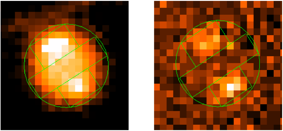
Figure 1: Jupiter’s images from the combined XMM-Newton EPIC cameras data ($\sim$1.4 side; left: 0.2$-$2 keV band; right: 3$-$10 keV) ; North is to the top, East to the left. Superposed are the regions used to extract auroral and low latitude disk lightcurves and spectra.

Periods when high particle background was affecting the data were identified from the lightcurve (top panel of Fig. 2, in 100 s bins) of $>$10 keV events detected over the common fields of view (30 diameter) of the EPIC-MOS and pn cameras combined. Excluding these intervals, which are evident in Fig. 2 at the beginning and/or end of each spacecraft orbit, leaves 210 ks of good quality data on which all subsequent analysis was carried out.

Figure 2: Jupiter’s lightcurves from the combined EPIC-pn and MOS cameras for the Nov. 2003 XMM-Newton observation. The gap of $\sim$60 ks centred at 1.5 $\times$ 10⁵ s into the observation is due to the spacecraft perigee passage between revs 0726 and 0727. ‘Full field’: $>$10 keV events from the whole field of view, in 100 s bins. ‘Disk’, ‘North aurora’ and ‘South aurora’ are the 0.2$-$2 keV low latitude disk emission, North and South auroral spots, respectively (from extraction regions in Fig. 1, in 5 min bins). ‘CML’: System III Central Meridian Longitude.

The 0.2$-$2 keV lightcurves (5 min bins) from the combined EPIC detectors for the disk and the auroral spots are shown in Fig. 2 (second, third and fourth panel from the top, respectively). The planet’s 10 hr rotation period is clearly visible in the lightcurve of the North and South auroral spots, but not so in the disk emission. The modulation appears to be stronger during the first XMM-Newton revolution, especially for the South aurora. Amplitude spectra generated from the data are shown in Fig. 3: a very significant peak, centred at 600 min, is present in both the North and South auroral spot power spectra (with clear sidelobes in the North spot, and beat peaks at 200 and 300 min); for the low latitude disk emission (Equator in Fig. 3) the level of power rises for periods longer than $\sim$300 min, but without the structure seen in the spots: this power may reflect some mixing (see Sect. 4) of auroral emission with the disk. There is a 10% decrease in the average soft X-ray flux from both aurorae between the first and the second spacecraft revolution; instead a 40% increase, noticeable in Fig. 2, takes place in the equatorial flux: this is found to be correlated with a similar increase in solar X-ray flux (see Bhardwaj et al. [2005] for a detailed study of the temporal behaviour of the low latitude disk emission, which appears to be controlled by the Sun). The bottom panel in Fig. 2 shows the System III Central Meridian Longitude (CML). The North spot is brightest around CML = 180^o, just like Chandra found in both Dec. 2000 and Feb. 2003 (Gladstone et al. [2002], Elsner et al. [2005]). The South spot peaks earlier than the North one by $\sim$90^o, i.e. by a quarter of the planet’s rotation, again similar to what seen by Chandra (Elsner et al. [2005]). Chandra also found the South auroral emission to extend in a band rather than being concentrated in a spot. It is hard to test this with XMM-Newton given its lower spatial resolution; the peaks in the lightcurve of the South spot, though, appear more diluted than those in the North in Fig. 2, which may be in line with a more spread-out emitting region.

Figure 3: Amplitude spectra generated from the lightcurves in Fig. 2

A search for periodic or quasi-periodic variability on short timescales in the auroral emissions, of the type observed by Chandra in Dec. 2000 and Feb. 2003, gives a null result (as for the Apr. 2003 XMM-Newton data; BR1): there is no evidence of any enhancement below 100 min in the amplitude spectra of Fig. 3. While it is possible that pulsations were simply absent in Jupiter’s aurorae at the time, we cannot exclude that the broader XMM-Newton Point Spread Function (PSF, $\sim$15 Half Energy Width, or HEW) with respect to that of the Chandra High Resolution Camera ($\sim$0.5) diluted the auroral X-ray emission with that from the planet’s low latitudes to the extent of masking any periodic (or quasi-periodic) behaviour. No periodic or quasi-periodic oscillations have been observed by Chandra in the low latitude disk emission of Jupiter (Bhardwaj et al. [2006a]) and none are found here.

3 EPIC spectral images

3.1 Emission line imaging

The first observation of Jupiter by XMM-Newton in Apr. 2003 (BR1) indicated that the auroral X-ray spectra can be modelled with a superposition of emission lines, including most prominently those of highly ionised oxygen (OVII, at 0.57 keV, and OVIII Ly$\alpha$, 0.65 keV). Instead, Jupiter’s low-latitude X-ray emission displays a spectrum consistent with that of solar X-rays scattered in the planet’s upper atmosphere; predominant components of this emission are lines from FeXVII transitions (at $\sim$0.7 and 0.8 keV) and MgXI (1.35 keV, BR1).

Fig. 4 displays EPIC images from the Nov. 2003 XMM-Newton observation in narrow spectral bands centred on the OVII, OVIII, FeXVII and MgXI lines: the OVII emission peaks clearly on the North and (more weakly) the South auroral spots, OVIII extends to lower latitudes, with an enhancement at the North spot, while MgXI and especially FeXVII display a more uniform distribution over the planet’s disk.

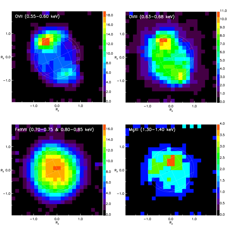
Figure 4: Smoothed XMM-Newton EPIC images of Jupiter in narrow spectral bands: From top left, clockwise: OVII, OVIII, Mg XI, Fe XVII. The colour scale bar is in units of EPIC counts. The image of the planet appears slightly smaller than in Fig. 1 because of the different colour contrast. A graticule showing Jupiter’s orientation with 30^o intervals in latitude and longitude is overlaid. The circular mark with a dot indicates the sub-solar point; the sub-Earth point is at the centre of the graticule.

3.2 High energy spectral components

Although most of the X-ray emission of Jupiter is confined to the 0.2$-$2 keV band, a search at higher energies has produced very interesting results. Fig. 1 (right) is an image of Jupiter in the 3$-$10 keV band, which shows the presence of high energy emission from the auroral spots, but not so from the planet’s disk. A more detailed view of the auroral contributions at different energies (in the bands 0.2$-$1, 1$-$3, 3$-$5 and 5$-$10 keV respectively) is given in Fig. 5. Interestingly, the South spot is brighter than the North spot above 3 keV.

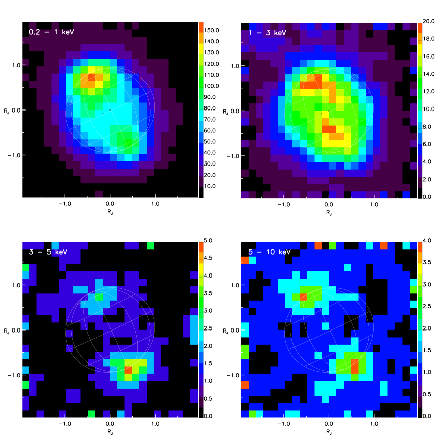
Figure 5: Smoothed XMM-Newton EPIC images of Jupiter in different bands extending to higher energies: From top left, clockwise: 0.2$-$1, 1$-$3, 5$-$10 and 3$-$5 keV. The colour scale bar is in units of EPIC counts. The image of the planet appears slightly smaller than in Fig. 1 because of the different colour contrast. A graticule is overlaid as in Fig. 4.

4 EPIC spectra

4.1 Extraction of the spectra

EPIC CCD data of Jupiter’s auroral zones and of the low-latitude disk emission suffer ‘spectral mixing’ due to the relatively broad XMM-Newton PSF ($\sim$15 HEW, practically independent of energy; see also BR1). Fig. 1 shows the regions used to extract the auroral and disk spectra, overposed to the EPIC images of Jupiter. We approached the task of separating the spectra of the different regions in two ways.

First we extracted spectra for the auroral regions, and then selected only sections of the corresponding lightcurves where the X-ray flux is higher than a given level. This is in practice phase spectroscopy, and results in selecting only phases where the spots are in maximum view, thus minimising contamination from the disk emission. By doing so we get insight to the shape of the true spectrum of the aurorae, but we artificially inflate the flux measurement, in a way that is difficult to correct; this is especially problematic because we want to combine all three EPIC cameras data to maximise the statistical quality of the spectra. Also, in order to extract the true disk emission without contamination by the aurorae, we ought to restrict the data selection to unrealistically short periods of the lightcurve (see Fig. 2).

Thus, for the proper spectral analysis we proceeded in a different way: we simulated the expected XMM-Newton image of Jupiter by convolving the XMM-Newton PSF at 0.5 keV (the planet’s X-ray emission peaks in the soft band) with the summed Chandra ACIS-S and HRC-I surface brightness distribution (Elsner et al. [2005]), and then calculated the number of events contributed to the XMM-Newton extraction boxes (this paper, Fig. 1); this procedure is justified because the relative strengths of the various spectral components do not vary very significantly over time. The same was done for events between 1.05 and 5 $\times$ 1.05 Jupiter radii from the planet’s centre in the ACIS image in order to get an estimate of the contribution of off-planet events to the XMM-Newton boxes (under the assumption that the background is similar for the two spacecraft). Knowing the total number of events in the Chandra selection regions, we could then calculate the percentage of events in each Chandra region that contribute to each XMM-Newton extraction box. The results are shown in Table 1. From this we see that we can expect mixing of disk and background events with auroral ones, and even a small amount of mixing of North and South events in the South and North boxes respectively. Using these results it has been possible to prescribe equations which recover the spectra for Jupiter’s three extraction regions. In order to maintain the ‘de-mixing’ task manageable, we only subtracted the appropriate fractions of disk and auroral spectra from the aurorae and disk respectively, and ignored the less significant contributions, i.e. mixing of off-planet background events and aurora-aurora contamination.

Table 1: Percentages of events from Chandra’s Jovian regions in the XMM-Newton extraction boxes

$\begin{array}[]{cccc}\hline\cr\hline\cr\vskip 3.0pt plus 1.0pt minus 1.0pt\cr{\it Chandra}^{\prime}s~{}region&\lx@intercol\hfil{\it XMM-Newton}~{}extraction~{}box\hfil\lx@intercol\\ \hline\cr&North~{}aurora&South~{}aurora&Disk\\ \hline\cr North~{}aurora&62.0&0.9&7.8\\ South~{}aurora&1.3&57.3&9.4\\ Disk&17.2&12.5&40.8\\ Off-planet~{}X-rays^{a}&1.1&0.8&1.5\\ \vskip 3.0pt plus 1.0pt minus 1.0pt\cr\hline\cr\hline\cr\end{array}$

^a Events falling between 1.05 and 5 $\times$ 1.05 Jupiter radii from the planet’s centre

We did not subtract the diffuse cosmic background from the spectra because Jupiter is foreground to it, nor the residual particle background, which is $<$1% of Jupiter’s flux in the band 0.2$-$2 keV. However, the particle background becomes a significantly higher fraction of the flux at higher energies. This is discussed in Sect. 4.2.

Fig. 6 shows a comparison of the North aurora EPIC-pn spectrum extracted with our first method (in black, ‘Phase spectroscopy’, selecting on time intervals when the X-ray flux is above 0.015 counts s^-1 in the EPIC-pn camera) and the latter ‘De-mixing’ (in red). The de-mixed spectrum has a lower flux because, correctly, is averaged over all flux levels of the source. The general shape is very similar, which suggests that our de-mixing stategy is working. So we used the de-mixed spectra throughout the following spectral analysis.

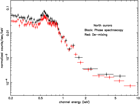
Figure 6: Comparison of the Nov. 2003 EPIC-pn spectra of the North aurora obtained with two different extraction techniques: ‘Phase spectroscopy’ (black) and ‘De-mixing’ (red). The overall shapes of the spectra are very similar, while the flux in the de-mixed spectrum is lower, as expected (see text for details).

4.2 North and South auroral spectra

Before starting detailed spectral fitting, we compared the spectra from the combined EPIC-pn and MOS-1 and -2 cameras, extending to the 10 keV upper bound of the instrumental responses, for Jupiter’s three extraction regions. We used the technique described in Page et al. ([2003]) to combine the spectra from the different cameras, and the corresponding response matrices; these, and the auxiliary response files, had been built using the SAS tasks rmfgen and arfgen with the point source option (following the technique used in BR1).

Fig. 7 shows the North and South spots and the low latitude disk spectra, after de-mixing: as first pointed out by BR1, there are clear differences in the shape of the spectra, with the auroral emission peaking at lower energy (0.5$-$0.6 keV) than the disk (0.7$-$0.8 keV). Emission features in the range 1$-$2 keV are visible in all the spectra, but are stronger in the disk (see Branduardi-Raymont et al. [2006] for a detailed analysis of the disk spectrum). The presence of a high energy component ($>$2 keV) from the aurorae is indeed confirmed, while this is missing in the disk emission. The 2$-$10 keV count rate is 6%, 14% and 5% of that in the 0.2$-$2 keV for North, South and equatorial regions respectively. The horizontal line in Fig. 7 represents the estimated level of the particle background for the combined EPIC cameras: the disk emission dips into it at $\sim$3 keV, while the signal from the aurorae is well above the line out to $\sim$7 keV. The EPIC particle background level was estimated from the analysis of Lumb ([2002]), and was verified for the Jupiter observation by examination of the flux measured in regions of the EPIC-MOS cameras outside the telescope field of view. This background is known to have an essentially flat distribution out to the highest energies (Lumb [2002]). Unfortunately we do not have a precise measurement of its level in the EPIC-pn camera during the Jupiter observation, which prevents us from subtracting it from the combined EPIC spectra. However, in the de-mixing process some 20$-$30% of the particle background is automatically taken away, so we do not expect the residual background to affect significantly our high energy results. In particular, the fits will be mostly constrained by the parts of the spectra with the highest signal to noise, i.e. by the low energy spectral channels.

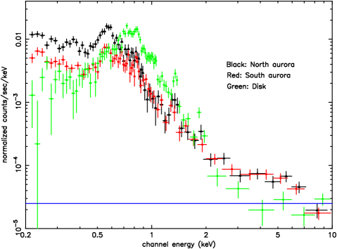
Figure 7: Combined Nov. 2003 EPIC spectra of the North (black) and South (red) aurorae, and of the low latitude disk (green) spectrum. Differences in spectral shape between auroral and disk spectra are clear. The presence of a high energy component in the spectra of the aurorae is very evident, with a substantial excess relative to the disk emission extending to 7 keV. The horizontal blue line shows the estimated level of the EPIC particle background.

4.3 Variability

Another issue to consider, in addition to the spectral complexity already discussed, is that of variability: we have already seen that the lightcurves in Fig. 2 show a 40% increase in the disk emission between XMM-Newton revs 0726 and 0727. Figs 8 and  9 show combined EPIC North and South auroral spectra respectively, accumulated separately over the two XMM-Newton orbits in Nov. 2003, together with the spectra from the Apr. 2003 observation (BR1). The latter have been re-analysed using the extraction regions in Fig. 1 and the de-mixing technique as for the Nov. 2003 data.

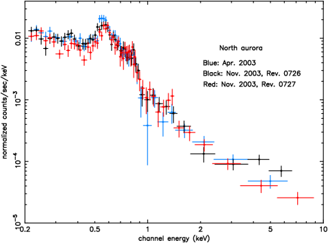
Figure 8: Combined EPIC spectra of the North aurora for the two separate XMM-Newton revolutions, 0726 (black) and 0727 (red), in Nov. 2003, and for the Apr. 2003 observation (blue).

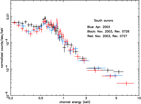
Figure 9: Combined EPIC spectra of the South aurora for the two separate XMM-Newton revolutions, 0726 (black) and 0727 (red), in Nov. 2003, and for the Apr. 2003 observation (blue).

The North and South auroral spectra from the three datasets have very similar overall shapes (this reinforces the validity of our spectral de-mixing). However, both North and South spectra from rev. 0726 show a larger flux (by a factor of $\sim$2) in the high energy component at 4$-$7 keV; also between 0.3 and 0.4 keV the flux appears higher (especially for the South aurora) than those in Apr. 2003 and Nov. 2003, rev. 0727: in fact, the spectra at these two epochs are remarkably similar to each other for both aurorae despite the seven month gap between them. We have checked the stability of the particle background level between the two Nov. 2003 revolutions in regions of the EPIC-MOS cameras outside the telescope field of view and conclude that the flux changes at high energy are intrinsic to the aurorae.

The trend of the auroral emission variability between the two Nov. 2003 XMM-Newton revolutions, with enhancements at both low and high energies in the first part of the observation, is opposite to that of the disk emission, which increases by 40% between revs 0726 and 0727 (Fig. 2). This is consistent with the idea that different mechanisms are responsible for the origin of the X-rays in the auroral and low latitude regions (BR1). Apart from the strong OVII emission line at 0.57 keV (BR1), features at $\sim$0.8 keV are visible in both North and South spectra, while a line at $\sim$1.35 keV, with variable strength, is clearly present only in the North. A MgXI line (actually a He-like triplet, unresolved at the EPIC resolution) appears at this energy in the solar coronal spectrum at times of strong activity (Peres et al. [2000]), suggesting that we are seeing some disk contamination in Jupiter’s aurorae.

4.4 Spectral fits

Given the detailed differences in the spectra collected at different times for the various regions, we analysed the two Nov. 2003 revolutions and re-analysed the Apr. 2003 data separately and then compared the results. We restricted spectral fitting of the auroral emissions to the 0.2$-$7 keV range, to minimise the possibility of particle background contamination becoming an issue. The spectra were binned so as to have at least 40 counts per channel, well above the limit at which the $\chi^{2}$ minimisation technique is applicable in the fits. These were carried out with XSPEC v. 11.3.2.

Following the original analysis of the Apr. 2003 observation (BR1), we started by fitting a combination of continuum models and emission lines to the auroral data of the Apr. 2003 and Nov. 2003, revs 0726 and 0727, individual datasets. Since we have used a different (and more accurate) spectral extraction technique and we are fitting also the high energy part of the spectra, which was ignored in the original analysis of the Apr. 2003 observations, we could expect to obtain results that slightly differ from those reported in BR1. We tried both thermal bremsstrahlung and power law models for the continuum, and we included four and five emission lines in our trials. We first left all model parameters free in the fits, and found that a two bremsstrahlung continuum is a better fit than a single bremsstrahlung or a single power law for all the datasets. In all cases four gaussian lines are required to explain the emission features: their best fit energies are 0.32, 0.57, 0.69 and 0.83 keV for the rev. 0726 spectra; in rev. 0727 and in Apr. 2003 the lowest energy line is not detected, but one is clearly present at 1.35 keV (probable disk contamination; see Sect. 4.3). The 90% confidence range for the 0.32 keV line is 0.23$-$0.37 and 0.21$-$0.35 keV for the North and South aurora respectively. We then fixed the line energies and widths at the best fit values (the line widths are smaller or comparable to the EPIC camera resolution of $\sim$100 eV FWHM) and refitted the data; in this way we limit the number of free parameters in fits with relatively small numbers of spectral bins and are able to achieve an estimate of the free parameters uncertainties. Table 2 lists best fit parameters and 90% confidence errors, and allows us to inspect the differences between the Nov. 2003, rev. 0726 spectra and those from the two other epochs: the former require much higher temperature bremsstrahlung continua in order to describe the excess at high energies; an emission line is also needed to explain a peak at 0.3$-$0.4 keV (the emission in this range is better modelled with a cooler bremsstrahlung continuum at the other two epochs), while, as already mentioned, a line at 1.35 keV is detected in Apr. and Nov. 2003, rev. 0727 only. The large errors, especially on the line equivalent widths, reflect the difficulty of constraining a complex model with relatively few spectral bins.

The very large 90% lower limits to the bremsstrahlung temperatures formally required for both aurorae in rev. 0726 (far exceeding the upper energy bound of the EPIC operational range), rather than measuring a physical quantity, simply indicate that the spectral slope is very flat. In fact, closer inspection of the Nov. 2003, rev. 0726 spectra with the best fit model overposed shows that the slope of the high energy tail is not properly fitted. A much better fit (in appearence, if not in the statistical sense, since the reduced $\chi^{2}$ values are below 1) is obtained substituting the high temperature bremsstrahlung with a flat power law (whose parameters are listed in Table 3). Figs 10 and  11 show the spectra and these best fits for the Nov. 2003, rev. 0726 observation of the North and South aurorae respectively.

Table 2: Best fit parameters (and their 90% confidence errors) for the 0.2$-$7 keV spectra of Jupiter’s auroral regions: thermal bremsstrahlung continua.

$\begin{array}[]{lcccc}\hline\cr\hline\cr\vskip 3.0pt plus 1.0pt minus 1.0pt\cr Nov.~{}2003$-$Rev.~{}0726&\lx@intercol\hfil North~{}aurora\hfil\lx@intercol&\lx@intercol\hfil South~{}aurora\hfil\lx@intercol\\ \chi^{2}/d.o.f.^{a}&\lx@intercol\hfil 37.4/42\hfil\lx@intercol&\lx@intercol\hfil 16.4/24\hfil\lx@intercol\\ Bremsstrahlung&kT^{b}&Norm^{c}&kT^{b}&Norm^{c}\\ \vskip 3.0pt plus 1.0pt minus 1.0pt\cr\hline\cr\vskip 3.0pt plus 1.0pt minus 1.0pt\cr Bremss.~{}1&0.27^{\rm+0.06}_{\rm-0.05}&49.8^{\rm+30.2}_{\rm-19.8}&0.34^{\rm+0.15}_{\rm-0.09}&16.9^{\rm+12.8}_{\rm-4.2}\\ Bremss.~{}2&\geq 50&\geq 2.9&\geq 80&\geq 3.7\\ \vskip 3.0pt plus 1.0pt minus 1.0pt\cr\hline\cr\vskip 3.0pt plus 1.0pt minus 1.0pt\cr Line~{}energy^{d}&Flux^{e}&EW^{f}&Flux^{e}&EW^{f}\\ \vskip 3.0pt plus 1.0pt minus 1.0pt\cr\hline\cr\vskip 3.0pt plus 1.0pt minus 1.0pt\cr 0.32&29.5^{\rm+10.6}_{\rm-5.0}&210^{\rm+70}_{\rm-40}&23.7^{\rm+7.4}_{\rm-7.6}&390^{\rm+120}_{\rm-130}\\ 0.57&10.9\pm 1.7&350\pm 60&5.6^{\rm+1.3}_{\rm-2.0}&360^{\rm+80}_{\rm-130}\\ 0.69&3.6\pm 1.0&230^{\rm+70}_{\rm-60}&2.2\pm 0.7&240\pm 80\\ 0.83&1.1^{\rm+0.5}_{\rm-0.4}&120\pm 50&0.9^{\rm+0.4}_{\rm-0.7}&160^{\rm+70}_{\rm-120}\\ \vskip 3.0pt plus 1.0pt minus 1.0pt\cr\vskip 3.0pt plus 1.0pt minus 1.0pt\cr\hline\cr\hline\cr\vskip 3.0pt plus 1.0pt minus 1.0pt\cr Nov.~{}2003$-$Rev.~{}0727&\lx@intercol\hfil North~{}aurora\hfil\lx@intercol&\lx@intercol\hfil South~{}aurora\hfil\lx@intercol\\ \chi^{2}/d.o.f.^{a}&\lx@intercol\hfil 55.4/48\hfil\lx@intercol&\lx@intercol\hfil 29.9/27\hfil\lx@intercol\\ Bremsstrahlung&kT^{b}&Norm^{c}&kT^{b}&Norm^{c}\\ \vskip 3.0pt plus 1.0pt minus 1.0pt\cr\hline\cr\vskip 3.0pt plus 1.0pt minus 1.0pt\cr Bremss.~{}1&0.10\pm 0.01&560^{\rm+220}_{\rm-80}&0.10\pm 0.01&270^{\rm+3610}_{\rm-110}\\ Bremss.~{}2&3.7^{\rm+1.7}_{\rm-1.0}&2.7\pm 0.4&13.5^{\rm+53}_{\rm-13.5}&1.9^{\rm+0.3}_{\rm-0.4}\\ \vskip 3.0pt plus 1.0pt minus 1.0pt\cr\hline\cr\vskip 3.0pt plus 1.0pt minus 1.0pt\cr Line~{}energy^{d}&Flux^{e}&EW^{f}&Flux^{e}&EW^{f}\\ \vskip 3.0pt plus 1.0pt minus 1.0pt\cr\hline\cr\vskip 3.0pt plus 1.0pt minus 1.0pt\cr 0.57&8.8^{\rm+1.0}_{\rm-1.4}&380^{\rm+40}_{\rm-60}&3.0^{\rm+1.0}_{\rm-0.8}&230^{\rm+80}_{\rm-60}\\ 0.69&6.2\pm 1.0&910\pm 150&3.6^{\rm+0.7}_{\rm-1.0}&420^{\rm+80}_{\rm-120}\\ 0.83&1.5^{\rm+0.6}_{\rm-0.5}&160^{\rm+60}_{\rm-50}&3.2^{\rm+0.6}_{\rm-0.7}&650^{\rm+120}_{\rm-140}\\ 1.35&0.2\pm 0.1&140\pm 70&0.2^{\rm+0.1}_{\rm-0.2}&180^{\rm+90}_{\rm-180}\\ \vskip 3.0pt plus 1.0pt minus 1.0pt\cr\vskip 3.0pt plus 1.0pt minus 1.0pt\cr\hline\cr\hline\cr\vskip 3.0pt plus 1.0pt minus 1.0pt\cr Apr.~{}2003&\lx@intercol\hfil North~{}aurora\hfil\lx@intercol&\lx@intercol\hfil South~{}aurora\hfil\lx@intercol\\ \chi^{2}/d.o.f.^{a}&\lx@intercol\hfil 29.6/34\hfil\lx@intercol&\lx@intercol\hfil 12.2/15\hfil\lx@intercol\\ Bremsstrahlung&kT^{b}&Norm^{c}&kT^{b}&Norm^{c}\\ \vskip 3.0pt plus 1.0pt minus 1.0pt\cr\hline\cr\vskip 3.0pt plus 1.0pt minus 1.0pt\cr Bremss.~{}1&0.12\pm 0.01&400^{\rm+630}_{\rm-70}&0.08\pm 0.02&780^{\rm+3550}_{\rm-650}\\ Bremss.~{}2&18.1^{\rm+40.0}_{\rm-12.6}&2.5^{\rm+2.1}_{\rm-0.5}&100^{\rm+140}_{\rm-60}&3.5^{\rm+2.0}_{\rm-0.6}\\ \vskip 3.0pt plus 1.0pt minus 1.0pt\cr\hline\cr\vskip 3.0pt plus 1.0pt minus 1.0pt\cr Line~{}energy^{d}&Flux^{e}&EW^{f}&Flux^{e}&EW^{f}\\ \vskip 3.0pt plus 1.0pt minus 1.0pt\cr\hline\cr\vskip 3.0pt plus 1.0pt minus 1.0pt\cr 0.57&12.9\pm 1.6&530\pm 70&3.8\pm 1.0&320\pm 80\\ 0.69&5.3^{\rm+0.9}_{\rm-1.0}&630\pm 120&3.3\pm 0.9&570\pm 160\\ 0.83&1.6\pm 0.5&390\pm 120&1.9\pm 0.7&310\pm 120\\ 1.35&0.1\pm 0.1&60^{\rm+130}_{\rm-60}&0.2\pm 0.2&210\pm 210\\ \vskip 3.0pt plus 1.0pt minus 1.0pt\cr\vskip 3.0pt plus 1.0pt minus 1.0pt\cr\hline\cr\hline\cr\end{array}$

^a $\chi^{2}$ value and degrees of freedom
^b Bremsstrahlung temperature in keV
^c Bremsstrahlung normalisation at 1 keV in units of 10^-6 ph cm^-2 s^-1 keV^-1
d Energy of the emission features in keV (fixed in the fits)
^e Total flux in the line in units of 10^-6 ph cm^-2 s^-1
f Line equivalent width in eV

Table 3: Best fit parameters (and their 90% confidence errors) for the 0.2$-$7 keV spectra of Jupiter’s auroral regions from Nov. 2003, rev. 0726 (high energy power law).

$\begin{array}[]{lcccc}\hline\cr\hline\cr\vskip 3.0pt plus 1.0pt minus 1.0pt\cr Nov.~{}2003$-$Rev.~{}0726&\lx@intercol\hfil North~{}aurora\hfil\lx@intercol&\lx@intercol\hfil South~{}aurora\hfil\lx@intercol\\ \chi^{2}/d.o.f.^{a}&\lx@intercol\hfil 29.2/42\hfil\lx@intercol&\lx@intercol\hfil 8.9/24\hfil\lx@intercol\\ Bremss./Powerlaw&kT^{b}/{\it\Gamma}^{c}&Norm^{d}&kT^{b}/{\it\Gamma}^{c}&Norm^{d}\\ \vskip 3.0pt plus 1.0pt minus 1.0pt\cr\hline\cr\vskip 3.0pt plus 1.0pt minus 1.0pt\cr Bremss.&0.40^{\rm+0.08}_{\rm-0.07}&25.9^{\rm+7.0}_{\rm-11.7}&0.58^{\rm+0.29}_{\rm-0.13}&11.0^{\rm+6.6}_{\rm-4.8}\\ Powerlaw&0.20^{\rm+0.19}_{\rm-0.17}&0.4^{\rm+0.2}_{\rm-0.1}&0.13^{\rm+0.19}_{\rm-0.12}&0.4^{\rm+0.6}_{\rm-0.1}\\ \vskip 3.0pt plus 1.0pt minus 1.0pt\cr\hline\cr\vskip 3.0pt plus 1.0pt minus 1.0pt\cr Line~{}energy^{e}&Flux^{f}&EW^{g}&Flux^{f}&EW^{g}\\ \vskip 3.0pt plus 1.0pt minus 1.0pt\cr\hline\cr\vskip 3.0pt plus 1.0pt minus 1.0pt\cr 0.32&37.9^{\rm+10.0}_{\rm-10.1}&410\pm 110&25.8^{\rm+6.5}_{\rm-7.0}&570^{\rm+140}_{\rm-160}\\ 0.57&12.2^{\rm+1.8}_{\rm-1.9}&490^{\rm+70}_{\rm-80}&5.7\pm 1.3&380\pm 90\\ 0.69&3.3^{\rm+1.0}_{\rm-0.9}&230^{\rm+70}_{\rm-60}&2.5\pm 0.8&280\pm 90\\ 0.83&1.2\pm 0.5&140\pm 60&0.7\pm 0.4&110\pm 70\\ \vskip 3.0pt plus 1.0pt minus 1.0pt\cr\vskip 3.0pt plus 1.0pt minus 1.0pt\cr\hline\cr\hline\cr\end{array}$

^a $\chi^{2}$ value and degrees of freedom
^b Bremsstrahlung temperature in keV
^c Power law photon index
^d Bremsstrahlung/Power law normalisation at 1 keV in units of 10^-6 ph cm^-2 s^-1 keV^-1
e Energy of the emission features in keV (fixed in the fits)
^f Total flux in the line in units of 10^-6 ph cm^-2 s^-1
g Line equivalent width in eV

Figure 10: XMM-Newton EPIC spectrum of Jupiter’s North aurora from the Nov. 2003, rev. 0726 observation, fitted with thermal bremsstrahlung and power law continua, plus four lines (see text for details).

Figure 11: XMM-Newton EPIC spectrum of Jupiter’s South aurora from the Nov. 2003, rev. 0726 observation, fitted with thermal bremsstrahlung and power law continua, plus four lines (see text for details).

Table 4 lists the 0.2$-$2.0 and 2.0$-$7.0 keV energy fluxes for both aurorae in Nov. 2003, revs 0726 and 0727, and in Apr. 2003. We first note that the fluxes derived for the two bremsstrahlungs and the bremsstrahlung + power law models (rev. 0726) are fairly similar, as one would expect since the fits are statistically equally good; the differences can be taken as an indication of the uncertainties affecting the results. While the North aurora is always between 60 and 90% brighter than the South in the 0.2$-$2 keV range, the two aurorae are comparable in flux in the 2$-$7 keV range: this is consistent with what we see in Fig. 5, where the South aurora even outshines the North in the range 3$-$5 keV. Finally, Table 4 confirms the factor of $\sim$2 decrease in strength of the high energy component in both aurorae between revs 0726 and 0727, while the Apr. 2003 level lies in between the two. The behaviour is different in the range 0.2$-$2 keV, where the energy flux of the North aurora is larger in rev. 0727, and both aurorae are brightest in Apr. 2003: this is at odds with the decrease by $\sim$10% observed in the lightcurves between revs 0726 and 0727 (Fig. 2 and Sect. 2), and probably reflects a change in spectral shape (Table 2). The combined North and South auroral luminosities in the 0.2$-$2 keV band are 0.48, 0.41 and 0.46 GW in Apr. and Nov. 2003, revs 0726 and 0727, respectively. As a comparison, in Feb. 2003 Chandra ACIS measured an X-ray luminosity of 0.68 GW from the North aurora in the energy range 0.3$-$1 keV (Elsner et al. [2005]).

Fig. 12 shows the high energy continuum model components fitted to the Nov. 2003 auroral data (flat power law for rev. 0726 and steeper bremsstrahlung for rev. 0727) and compares them with the predictions of Singhal et al. ([1992]) for bremsstrahlung emissions by electrons with characteristic energies between 10 and 100 keV. The bremsstrahlung fits of rev. 0727 for both the North and South aurorae lie remarkably close to the predicted spectra; the same is true for the models fitted to the Apr. 2003 data, which are not shown to avoid making the diagram too crowded. The models for rev. 0726, however, are very much at variance with the predictions, and suggest a very different electron distribution for both aurorae. For all datasets (Apr. and Nov. 2003) essentially all the observed flux at $>$2 keV (and a maximum of 10% of that between 0.2 and 2 keV) is accounted for by the high energy auroral components. The combined North and South auroral luminosities in the 2$-$7 keV band are 58, 90 and 38 MW for the Apr. and Nov. 2003, revs 0726 (power law fit) and 0727, respectively.

We have also searched for the presence of a high energy component in the Chandra ACIS spectra of 2003, Feb. 24$-$26 (Elsner et al. [2005]): a weak, but significant signal is detected in the band 2$-$7 keV, with flux in the range 1.9$-$3.2 $\times$ 10^-14 erg cm^-2 s^-1 (for the two Chandra orbits respectively), corresponding to a luminosity of 52$-$88 MW for both North and South aurorae combined.

From extrapolation of the best fit spectral models in Tables 2 and 3 we can estimate the X-ray flux and thus the emitted luminosity in the aurorae at higher energies; in particular we can compare with the predictions of Waite et al. ([1992]) and the upper limits determined by Hurley et al. ([1993]) with the Ulysses Gamma Ray Burst (GRB) instrument in the 27$-$48 keV band. If we adopt the best fit values of bremsstrahlung temperature and normalisation found for rev. 0727, the combined output of the North and South aurorae in the 27$-$48 keV range corresponds to a luminosity of 4.3 MW: this compares well with Waite et al. ([1992]) most optimistic prediction of 3.3 MW and is consistent with the GRB most stringent upper limit ($<$ 100 MW) (Hurley et al. [1993]). If instead we extrapolate the Apr. 2003 best fit, we obtain a luminosity $\sim$10 times larger, still consistent with the Hurley et al. upper limits. Using the best fit parameters for rev. 0726, extrapolation of the very flat power law leads to a luminosity $\sim$2 GW, clearly in excess of predictions and upper limits. This extreme result, however, could be mitigated if the spectral slope (determined over the narrow energy band 2$-$7 keV), and thus the electron energy distribution, has a downturn below $\sim$50 keV.

Table 4: X-ray fluxes from Jupiter’s aurorae in the energy ranges 0.2$-$2.0 and 2.0$-$7.0 keV for the three available XMM-Newton datasets. For rev. 0726 fluxes are reported for both two-bremsstrahlung and bremsstrahlung + power law fits.

$\begin{array}[]{lccc}\hline\cr\hline\cr\vskip 3.0pt plus 1.0pt minus 1.0pt\cr&&\lx@intercol\hfil Flux^{a}\hfil\lx@intercol\\ \vskip 3.0pt plus 1.0pt minus 1.0pt\cr\hline\cr\vskip 3.0pt plus 1.0pt minus 1.0pt\cr&Energy~{}range&North~{}aurora&South~{}aurora\\ &({\rm keV})&&\\ \vskip 3.0pt plus 1.0pt minus 1.0pt\cr\hline\cr\vskip 3.0pt plus 1.0pt minus 1.0pt\cr Nov.~{}2003,~{}rev.~{}0726&0.2$-$2.0&6.1&3.7\\ Two~{}brem.&2.0$-$7.0&0.8&0.9\\ \vskip 3.0pt plus 1.0pt minus 1.0pt\cr\hline\cr\vskip 3.0pt plus 1.0pt minus 1.0pt\cr Nov.~{}2003,~{}rev.~{}0726&0.2$-$2.0&5.9&3.6\\ Brem.~{}+~{}power~{}law&2.0$-$7.0&1.0&1.1\\ \vskip 3.0pt plus 1.0pt minus 1.0pt\cr\hline\cr\vskip 3.0pt plus 1.0pt minus 1.0pt\cr Nov.~{}2003,~{}rev.~{}0727&0.2$-$2.0&7.0&3.7\\ Two~{}brem.&2.0$-$7.0&0.4&0.5\\ \vskip 3.0pt plus 1.0pt minus 1.0pt\cr\hline\cr\vskip 3.0pt plus 1.0pt minus 1.0pt\cr Apr.~{}2003&0.2$-$2.0&7.9&4.5\\ Two~{}brem.&2.0$-$7.0&0.7&0.8\\ \vskip 3.0pt plus 1.0pt minus 1.0pt\cr\hline\cr\hline\cr\end{array}$

^a Flux in units of 10^-14 erg cm^-2 s^-1

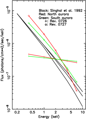
Figure 12: High energy model components fitted to the Nov. 2003 auroral data, compared with Singhal et al. ([1992]) bremsstrahlung X-ray flux predictions for three characteristic electron energies (10, 30 and 100 keV, from bottom to top curve). The Apr. 2003 models lie close to the predictions and are not shown to avoid crowding the diagram.

4.5 Combined Apr. and Nov. 2003 spectra

In an attempt to establish more accurately the energy, and thus the origin, of the soft X-ray line present in the EPIC spectra at $\sim$0.3 keV, we first combined all the data of the North aurora from the two observing campaigns, then we combined the South aurora data with them too (using the technique described by Page et al. [2003]; Sect. 4.2), and analysed the resulting spectra. In the first case (all data for the North aurora) we find a best fit line energy of 0.32 keV, and in the second (North and South aurorae combined) of 0.30 keV. Even with the increased signal-to-noise ratio of the data, it is very difficult to establish the energy of the feature securely. Figs 8 and 9 show that there are changes in the shape of the low energy spectrum over the datasets, especially in the South aurorae, which contribute to the uncertainty of the results. As a final trial, we combined the North and South aurora data for the individual epochs and re-fitted, obtaining a best fit energy of 0.31${}^{\rm+0.03}_{\rm-0.06}$, 0.30${}^{\rm+0.03}_{\rm-0.08}$ and 0.30${}^{\rm+0.01}_{\rm-0.06}$ keV for Apr. and Nov. 2003, revs 0726 and 0727, respectively. Thus, only by combining both auroral spectra can we detect the line in two of the three datasets. The best fit model for rev. 0726 in the range 0.2$-$2 keV is shown in Fig. 13. We conclude that the results of the analysis of the Nov. 2003 data and of the re-analysis of those from Apr. 2003 are more consistent with SXI (0.32 keV) or SXII (0.34 keV) transitions than CVI (0.37 keV), although only data at higher sensitivity and spectral resolution will provide the definite answer and separate the ion species involved.

Figure 13: XMM-Newton EPIC spectrum of Jupiter’s North and South aurorae combined from the Nov. 2003, rev. 0726 observation.

5 RGS spectra

After re-registration to Jupiter’s frame of reference, good quality RGS data from the Nov. 2003 XMM-Newton observation were selected by excluding intervals of high background from further analysis. Fig. 14 shows the spectrum of Jupiter obtained by combining the RGS1 and 2 first order data from both XMM-Newton revolutions in Nov. 2003: along the vertical axis is the spatial distribution of the emission in the cross dispersion direction (colour coded according to the detected flux), while X-ray wavelength is plotted along the horizontal axis. Because the cross dispersion coordinate for every event is referred to spacecraft on-axis, and Jupiter was 25 off-axis during the observation, its centre is shifted downwards from the zero level by the same amount. The RGS clearly separates the emission from OVII (the triplet at 21.6$-$22.1 Å, or 0.56$-$0.57 keV), OVIII Ly$\alpha$ (19.0 Å, or 0.65 keV) and FeXVII (15.0 and $\sim$17.0 Å, or $\sim$0.73 and 0.83 keV).

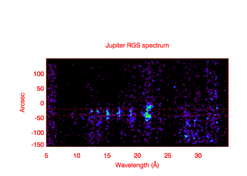
Figure 14: RGS spectrum of Jupiter from the combined RGS1 and 2 datasets (first order only) of both XMM-Newton revolutions in Nov. 2003. Y-axis: Spatial extent of the emission in the cross dispersion direction (colour coded such that light blue and green represent brighter pixels); x-axis: X-ray wavelength. The two dashed horizontal lines mark the approximate location of Jupiter’s aurorae (the planet’s N$-$S axis is essentially perpendicular to the RGS dispersion direction, with N at the bottom of the figure).

Interestingly, the RGS spectrum also shows evidence for the different spatial extension of the line emitting regions, in agreement with the EPIC spectral mapping of Fig. 4: OVII photons are well separated spatially into the two aurorae, while the other lines are filling in the low latitude/cross dispersion range. In particular, this is true for the FeXVII lines at 15 and 17 Å, which are known to be associated with the planet’s disk and are thought to be scattered solar X-rays (BR1, Maurellis et al. [2000], Cravens et al. [2006]). Unfortunately, the combination of lower RGS sensitivity and low source flux at the short and long wavelength ends of the instrument operational range is such that Jupiter’s spectrum is only significantly detected in the range 13$-$23 Å (0.54$-$0.95 keV), to which we have restricted subsequent spectral fitting.

Spectral distributions were extracted using the SAS task rgsspectrum, which selects source and background events from spatial regions adjacent in cross-dispersion direction. Since Jupiter is an extended source (although small enough not to degrade the RGS energy resolution significantly) the selection area for its spectrum was augmented (from the standard value of 90%) to include 95% of the RGS PSF in the cross-dispersion direction, corresponding to a size of 87 on the sky. No background subtraction was carried out, as in the EPIC case, because Jupiter is a foreground object. After the spatial selection is carried out, rgsspectrum applies the RGS dispersion relation to further select true X-ray photons on the basis of their CCD energy values. RGS1 and 2 first order spectra, and corresponding matrices, were then combined according to the same procedure followed for the EPIC spectra (Sect. 4.2). The final spectrum was grouped by a factor of 3, resulting in channels $\sim$30 mÅ wide, which still sample well the RGS resolution of $\sim$70 mÅ FWHM. Modelling of the RGS spectrum was carried out with SPEX 2.00.11 (Kaastra et al. [1996]).

We started by adopting a composite model including a plasma in collisional ionisation equilibrium (to represent Jupiter’s disk emission and account in particular for the FeXVII line emission), a thermal bremsstrahlung component and gaussian emission lines at the wavelengths of the OVII triplet and OVIII Ly$\alpha$ (to account for the auroral emission from ion charge exchange): this falls short of explaining the broad wings of the oxygen lines, which are clearly evident in the RGS data (blue crosses) shown in Figs 15 and 16. Only by adding two broad gaussian components centred on the OVII and OVIII emissions can we achieve an acceptable fit. In the final best fit ($\chi^{2}$ = 360 for 280 d.o.f.) we also included gaussian lines corresponding to higher order OVII and OVIII transitions, to help modelling some residual emission still un-accounted for.

The only parameters left free to vary in the fit were the normalisations of all the model components, and the wavelengths and widths of the broad gaussians. The temperature of the disk plasma was fixed at 0.41 keV, which is the average of the values measured over the two XMM-Newton revolutions in Nov. 2003 (Branduardi-Raymont et al. [2006]), and the bremsstrahlung temperature was set to 0.2 keV, again the average measured by EPIC over the two revolutions for the North and South aurorae (Table 2). Since the fits are insensitive to altering the intrinsic widths of the narrow gaussian lines, these were fixed at 0.1 Å (the planet’s spatial extension broadens the lines by $\sim$80 mÅ). Table 5 lists the best fit values and the 1$\sigma$ r.m.s. errors for the line fluxes and the wavelengths and widths of the broad gaussians. The wavelength of the OVII broad component is consistent with that of the intercombination line, while the centre of the OVIII broad line is shifted to the red of that of the narrow line by 0.3 Å (corresponding to a speed of $\sim$4500 km s^-1). The FWHM widths of the two lines correspond to $\sim$9000 and 11000 km s^-1 for the OVII and OVIII emissions respectively. We have searched for possible changes in the centroids of the oxygen features as the aurorae move in and out of view, to try and investigate their dynamics further, but unfortunately the data signal-to-noise is too low.

Table 5: Best fit parameters for the auroral lines (narrow and broad) in the RGS spectrum of Jupiter. The errors are 1$\sigma$ r.m.s. The reference frame wavelengths and energies of the FeXVII lines and the MgXI triplet from the planet’s disk are also listed for comparison.

$\begin{array}[]{lcccc}\hline\cr\hline\cr\vskip 3.0pt plus 1.0pt minus 1.0pt\cr Line~{}id.&Line~{}wavelength^{a}&Line~{}energy^{b}&Flux^{c}&FWHM^{d}\\ \vskip 3.0pt plus 1.0pt minus 1.0pt\cr\hline\cr\vskip 3.0pt plus 1.0pt minus 1.0pt\cr OVII(r)^{e}&21.602&0.574&1.5^{\rm+2.3}_{\rm-1.5}&0.1\\ OVII(i)^{f}&21.807&0.568&0.2^{\rm+2.9}_{\rm-0.2}&0.1\\ OVII(f)^{g}&22.101&0.561&2.0^{\rm+2.1}_{\rm-1.9}&0.1\\ OVIIILy\alpha&18.970&0.654&0.0+0.4&0.1\\ OVIIILy\beta&16.006&0.775&0.5^{\rm+0.6}_{\rm-0.5}&0.1\\ OVIIILy\gamma&15.176&0.817&3.6\pm 0.9&0.1\\ OVIIILy\delta&14.821&0.836&0.5^{\rm+0.8}_{\rm-0.5}&0.1\\ OVIIHe\beta&18.627&0.666&0.9^{\rm+0.8}_{\rm-0.9}&0.1\\ OVIIHe\gamma&17.768&0.698&1.1\pm 0.6&0.1\\ OVIIHe\delta&17.396&0.713&0.9\pm 0.6&0.1\\ OVII~{}broad&21.80\pm 0.08&0.569\pm 0.002&20.6^{\rm+4.9}_{\rm-6.7}&0.68^{\rm+0.20}_{\rm-0.15}\\ OVIII~{}broad&19.26^{\rm+0.14}_{\rm-0.20}&0.644^{\rm+0.006}_{\rm-0.005}&6.0^{\rm+3.1}_{\rm-2.3}&0.71^{\rm+0.34}_{\rm-0.30}\\ FeXVII&15.015&0.826&&\\ FeXVII&15.262&0.812&&\\ FeXVII&16.776&0.739&&\\ FeXVII&17.074^{h}&0.726&\\ MgXI(r)^{e}&9.169&1.352&\\ MgXI(i)^{f}&9.230&1.343&\\ MgXI(f)^{g}&9.314&1.331&&\\ \vskip 3.0pt plus 1.0pt minus 1.0pt\cr\vskip 3.0pt plus 1.0pt minus 1.0pt\cr\hline\cr\hline\cr\end{array}$

^a Wavelength of the emission line in Å (fixed in the fits, except for the broad components)
^b Energy of the emission line in keV (fixed in the fits, except for the broad components)
^c Total flux in the line in units of 10^-6 ph cm^-2 s^-1
d FWHM width of the gaussian model in Å (fixed in the fits, except for the broad components)
^e Resonance line of the triplet
^f Intercombination line
^g Forbidden line
^h Average of two lines separated by 0.045 Å 

Fig. 15 shows the combined RGS spectrum and the best fit model derived above, while Fig. 16 displays the data and only the disk model component.

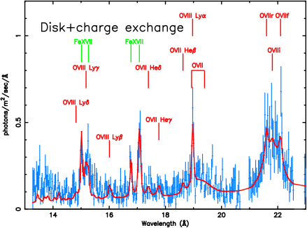
Figure 15: Combined RGS1 and 2 spectrum of Jupiter (blue crosses) with the best fit model (shown in red; see text for details).

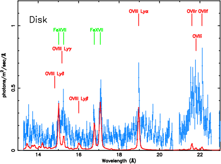
Figure 16: Combined RGS1 and 2 spectrum of Jupiter (blue crosses) with the best fit disk model component only (shown in red; see text for details).

Visual comparison of the RGS spectrum and of the model fits in Figs 15 and 16 provides interesting insights. The RGS clearly resolves the two FeXVII lines at 15.01 and 15.27 Å, and those at 16.77 and 17.10 Å. The flux observed around the 15.27 Å line is much larger than predicted from the disk only spectrum, so the fit forces an unrealistically large contribution from OVIII Ly$\gamma$ (15.18 Å) compared to those of lower order OVIII transitions. Letting the disk temperature free in the fit drives it to a higher value (0.66 keV) but does not alleviate the problem. Examination of the individual RGS spectra from revs 0726 and 0727 indicates that the flux at 15.27 Å was about a factor of two larger in the latter, suggesting that variability may be contributing to the discrepancy, since the disk component was modelled with the spectrum averaged over the two revolutions.

There is some evidence that the OVII triplet may be resolved, with high flux points at the locations of the resonance (21.60 Å) and forbidden (22.10 Å) lines, but the profile is complicated by the presence of the broad component which may be filling in between the two lines.

The narrow OVIII Ly$\alpha$ emission appears to be completely accounted for in the disk spectrum, so that we only derive an upper limit for any additional gaussian contribution of auroral origin (Table 5). For the strong auroral OVII emission at $\sim$22 Å, however, the situation is reversed: the disk contribution (Fig. 16) is very small, so essentially all the emission must be produced by charge exchange in the aurorae.

Because of the spatial extent of Jupiter emission in the RGS cross dispersion dimension, we can try and extract more information on the different spectral components by comparing the spectra obtained selecting spatial bands of different cross dispersion width.

Figure 17: Combined RGS 1 and 2 spectrum of Jupiter for different widths of the spatial extraction region in the cross dispersion dimension (half width of 8, 26 and 43 from bottom to top).

Fig. 17 shows the combined RGS1 and 2 spectra extracted over bands of cross dispersion half width of 8, 26 and 43 from bottom to top respectively; the narrowest band is expected to be dominated by the disk spectrum, while the largest one will contain both, disk and auroral emissions. Some interesting differences are apparent: the profile of the OVII triplet from the narrowest band peaks at the position of the resonance line (21.6 Å) while in both the larger bands the profile is more flat-topped, suggesting a more significant contribution by the forbidden line in the aurorae. The strength, and in particular the width, of the OVIII line at 19 Å increase dramatically by widening the extraction region, as more of the aurorae are included, while the appearence of the disk Fe lines is very similar in all regions, suggesting that the emission must be concentrated predominantly in the inner, narrower extraction band.

6 Discussion

Our XMM-Newton observations of the auroral X-ray emissions of Jupiter provide important new insights in the physical phenomena taking place on the planet, in its interactions with the magnetospheric plasma that surrounds it and in the effects that solar activity has on them. We summarise and discuss our main findings in the following sections, separating the ion and electron components which dominate at the low and high energy ends of the EPIC spectra respectively, and which are found to be variable. We conclude with a discussion of the RGS data and their implications.

6.1 The ion component

The EPIC spectra from Nov. 2003 and the re-analysis of the Apr. 2003 data confirm most of the results of BR1: the soft X-ray (0.2$-$2 keV) emission of Jupiter’s aurorae is best modelled by a continuum and the superposition of emission lines, which are most likely to be produced by energetic ions undergoing charge exchange as they precipitate in the planet’s upper atmosphere. We confirm that the majority of the emission in all spectra at both epochs emerges from OVII transitions at 0.57 keV ($\sim$22 Å). The underlying continuum, which we fit with a 0.1$-$0.3 keV bremsstrahlung model, may also be the result, at least in part, of line blending, by analogy with the X-ray emission observed from comets (Dennerl et al. [2003], Kharchenko et al. [2003]). Unlike comets, however, the origin of the ions, if solar wind or Jupiter’s magnetosphere, or both, is still a matter of debate.

Four other lines are detected in the EPIC spectra, but not all in all spectra. The best fit energies (Table 2) point to transitions of: a) SXI$-$SXII (0.32 keV; see discussion in Sect. 4.5); b) OVIII Ly$\alpha$ blended with higher orders of OVII (0.69 keV; see Table 5 for line energies); c) Higher orders of OVIII, possibly contaminated by some FeXVII emission (0.83 keV; see Table 5 and discussion of the excess emission at the FeXVII 15.27 Å line in Sect. 5); d) MgXI (1.35 keV; Table 5). Apart from the different (but still tentative) identification of the 0.32 keV line, the others are consistent with the interpretations given by BR1.

Recently, Kharchenko et al. ([2006]) have modelled the X-ray spectrum produced by energetic sulphur and oxygen ions precipitating into the Jovian atmosphere and compared it to those observed by Chandra and XMM-Newton, finding satisfactory agreement. We recall here that both the studies by Cravens et al. ([2003]) and Bunce et al. ([2004]) are able to explain Jupiter’s X-ray auroral emission by ions either from the planet’s magnetosphere or the solar wind, given appropriate acceleration is in place. A pure solar wind scenario, however, may be excluded by the excessive intensity of Ly$\alpha$ emission expected by protons also undergoing acceleration and precipitating in the atmosphere (Cravens et al. [2003]). While our present results still cannot resolve the dicothomy, we conclude that, also by analogy with the Earth, both magnetospheric and solar wind ions may well play a part in the process. In the case of the Earth it has not yet been possible to show conclusively that ion precipitation (whether of magnetospheric or solar wind origin) produces X-rays in the aurorae. However, recent work by Bhardwaj et al. ([2006c]), who have used the Chandra HRC-I to make the first soft X-ray observations of the Earth’s aurorae, has provided evidence for electron bremsstrahlung emission at energies below 2 keV.

The MgXI line at 1.35 keV is detected in Apr. 2003 and only in rev. 0727 in Nov. 2003. The line is likely to be residual contamination by the disk emission, which may become more evident above $\sim$1 keV where the ion contribution to the auroral emission is decreasing rapidly. We know that the disk acts as a mirror for solar X-rays (Maurellis et al. [2000], Cravens et al. [2006]): Bhardwaj et al. ([2005]) have shown that a very large solar flare took place at a time such that Jupiter’s response to it would have been observable by XMM-Newton had it not been switched off during perigee passage between revs 0726 and 0727. Possibly part of this response to the flare, Jupiter’s disk emission is seen to be overall brighter by $\sim$40%, and the flux of the MgXI line from the disk to be three times larger, in rev. 0727 than in rev. 0726 (Branduardi-Raymont et al. [2006]). The enhancement in the FeXVII 15.27 Å mentioned in Sect. 5 takes place at the same time as this brightening of the disk.

6.2 High energy electron component

A major, novel result of our analysis of Jupiter’s EPIC spectra is the discovery of a high energy continuum component which dominates the emission above $\sim$2 keV. The flux in this component, for both aurorae, is practically the same in Apr. and Nov. 2003, rev. 0727, while it is much higher (by more than a factor of 2 at $\sim$4 keV in the North aurora; Fig. 8) in rev. 0726. Thus the trend of the variability at energies above 2 keV is exactly opposite to that of the disk emission, which increases between the two revolutions. The spectral shape of the high energy component is best approximated by a thermal bremsstrahlung model when the flux is low, and by a very flat power law when it is brighter. A bremsstrahlung emission mechanism is expected to involve electrons, precipitating over the poles in Jupiter’s upper atmosphere and also likely to be responsible for the main ‘UV auroral oval’, which lies at lower latitudes (or L values) than the polar cap emission. This scenario is supported by another XMM-Newton result. We have already pointed out how the high energy component in the South aurora appears to be substantially brighter than in the North relative to the soft part of the spectrum (Fig. 5 and Table 4). We suggest that this reversal of brightness could be due to the larger offset of the North magnetic pole from Jupiter’s rotation axis (Gladstone et al. [2002]), which provides better sampling of the soft X-ray ion emission over the rotation period than at the South pole. Alternatively, or in conjunction with this, the South auroral oval is always much closer to the limb than the large, offset North auroral oval is, so from Earth we have a better chance of seeing emissions at 90^o to the electron deceleration direction. For this same reason the emissions seem to move out towards the limb at higher energy (Fig. 5): when the auroral regions are on the disk, the precipitating electrons are moving away from us, making it hard to see the bremsstrahlung emission they are producing. At or beyond the limb, the electrons are moving at more or less 90^o to us, i.e. in the direction at which the bremsstrahlung emission is at its peak.

The significant change in spectral slope between the two XMM-Newton revolutions (over a timescale of a couple of days) implies a severe hardening in the electron energy distribution with increasing flux: our spectral fits indicate characteristic electron energies of tens of keV, which, interestingly, are consistent with those implied for the precipitating electrons producing the cusp/polar cup FUV emissions on Jupiter (Bhardwaj and Gladstone [2000]). The change from a thermal to a non-thermal X-ray spectrum also suggests a substantial event has taken place to modify the basic character of the electron distribution.

Bremsstrahlung X-ray emission from primary electrons with a Maxwellian energy distribution, producing secondaries by ionisation in Jupiter’s upper atmosphere, has been predicted at very similar flux levels and very similar characteristic energies to those we observe in rev. 0727 (Waite [1991], Singhal et al. [1992] and Fig. 12). Thus our XMM-Newton observations of Jupiter have finally revealed what researchers have been speculating upon for more than a decade. The dramatic change in slope of the X-ray continuum above 2 keV between revs 0726 and 0727 suggests that the primary electron energy distribution may be the one mostly implicated in the variability. We note that at the same time a change occurs in the shape of the low energy spectra, attributed to ion emission (including the appearence of a line at $\sim$0.3 keV; Figs 8 and 9 and Table 2), so one can speculate that whatever affects the electrons may affect the ions too. Variability of this kind may follow a change in the plasma acceleration mechanism within Jupiter’s magnetosphere: large electric potentials are needed to accelerate the electrons and to explain the presence of the high energy stripped ions required for the charge exchange production of the auroral soft X-ray emission. This scenario has been studied in detail by Bunce et al. ([2004]) in the context of their model of pulsed magnetic reconnection at the dayside magnetopause between magnetospheric and magnetosheath field lines: they predict average potentials of $\sim$100 kV and 5 MV for electrons and ions respectively in their solar wind ‘fast flow’ case, appropriate to high density, high field solar wind conditions. The very different levels of potential required to accelerate the two particle populations could explain why in rev. 0726 the electron variability is much more marked than that of the ions.

A period of a couple of months of very strong solar activity began at the end of October 2003, with a rare ’Sun quake’ event (Donea and Lindsey [2005]), typical of the decaying phases of the solar cycle. Compression of Jupiter’s magnetosphere by energetic solar events is expected to result in the generation of potentials and currents leading to stronger acceleration of the ion and electron plasma inside it, which in turn can energise more powerful auroral emissions. Interestingly, about eight days before the XMM-Newton rev. 0726 observation took place, a large enhancement in solar wind electron, proton and ion fluxes was recorded by ACE, which orbits in the vicinity of the Sun-Earth L1 point (e.g. Skoug et al. [2004]). The solar ejecta causing this event are expected to have reached Jupiter around the time of our observation, if they were travelling at 1000 km s^-1 (this is a highly uncertain calculation, though, depending on the relative geometry of Jupiter and Earth, on the ejecta propagation direction and on the variable speed of the solar wind). In conclusion, the auroral phenomena may ultimately be solar-driven at some level, even if the emitting ions/electrons are not directly injected by the solar wind, and if we do not find strict correlations with solar behaviour. For example, solar activity immediately preceding the XMM-Newton observations in Apr. 2003 was at a lower level than in Nov. 2003. Nevertheless, a high energy auroral component was present in the spectra, and with a larger flux than in Nov. 2003 rev. 0727.

6.3 RGS results

The RGS spectrum enables us to resolve some of the blend of lines observed in Jupiter’s EPIC data into the dominant auroral emission contributions of OVII and OVIII ions, and those of FeXVII (15.0 and $\sim$17.0 Å) originating from the planet’s disk. Moreover, broad components of the OVII and OVIII lines are revealed for the first time. Their widths imply speeds of the order of $\pm$5000 km s^-1, which correspond to energies of $\sim$2.5 MeV for oxygen ions. This is not far off the level of energies required by the models of Cravens et al. ([1995], [2003]; 1 MeV/amu for magnetospheric ions, or 100 keV/amu for solar wind ions) and those implied by the potentials calculated by Bunce et al. ([2004]), suggesting that we are indeed seeing a population of accelerated ions precipitating from Jupiter’s outer magnetosphere to the polar caps. Since the observed oxygen line widths correspond to velocities along the line of sight, the total ion energies may accommodate a magnetospheric as well as a solar wind origin.

Despite the large errors on their fluxes (Table 5), it is clear, also from inspection of Figs 15 and 17, that the auroral OVII resonance and forbidden lines have similar strengths; this may seem at variance with expectations, considering Jupiter’s H₂ atmospheric density in the auroral regions: collisional de-excitation would most likely occur before the OVII ions had time to decay through the forbidden transition. However, as shown by Kharchenko and Dalgarno ([2000]), some of the brightest lines to emerge following charge transfer collisions are indeed from forbidden transitions of helium-like oxygen ions, which is consistent with our findings.

7 Conclusions

We have presented the analysis of Jupiter’s auroral X-ray emissions as observed over two XMM-Newton revolutions in Nov. 2003 and we have compared the results with those from an earlier observation in Apr. 2003 (BR1). The majority of the earlier results are confirmed, and in particular that ion charge exchange is likely to be responsible for the soft X-ray emission, with OVII providing the dominant contribution.

A major outcome of the present work is the discovery of a high energy X-ray bremsstrahlung component in the aurorae, a component which had been predicted but had never been detected for the lack of sensitivity of previous X-ray missions. The bremsstrahlung interpretation is supported by both spectral and morphological considerations. Moreover, we find that this component varied significantly in strength and spectral shape over the course of the Nov. 2003 observation. We suggest that the variability may be linked to the strong solar activity taking place at the time, and may be induced by changes in the potentials, and thus the acceleration mechanism, inside Jupiter’s magnetosphere. This could, to a lower degree, affect the ions too. As far as the question of the origin of the ions, we still cannot resolve the species responsible, if sulphur (likely to be of magnetospheric origin), or carbon (from the solar wind). It is conceivable that both scenarios play a role in what is certainly a very complex planetary structure.

The XMM-Newton RGS data add a new dimension to this study in that they allow us to examine the X-ray spectrum of the whole planet at high resolution for the first time. We clearly separate iron emission lines originating at low latitude on the disk of Jupiter from the bright oxygen lines most likely produced by charge exchange in the aurorae. The latter are found to be broad, implying that the ions are travelling with speeds (of the order of 5000 km s^-1) consistent with the levels of acceleration predicted by models recently developed to account for Jupiter’s auroral processes.

The data presented in this paper give an important contribution to the understanding of the physical environment where auroral emissions on Jupiter are generated: they show a good degree of consistency with theoretical models developed in recent years, and thus give us confidence that we broadly understand the basic processes powering Jupiter’s aurorae. Yet, the details are far from clear, such as those of the complex relationships between ion and electron populations in Jupiter’s magnetospheric environment, and the way these react to external influences such as solar activity. Given the limitations of current X-ray observations carried out remotely, in-situ measurements, also in the X-ray band, from future planetary missions will offer a very promising way forward.