Periodic radial velocity variations in RU Lupi

Abstract

Context. RU Lup is a Classical T Tauri star with unusually strong emission lines, which has been interpreted as manifestations of accretion. Recently, evidence has accumulated that this star might have a variable radial velocity.

Aims. We intended to investigate in more detail the possible variability in radial velocity using a set of 68 high-resolution spectra taken at the VLT (UVES), the AAT (UCLES) and the CTIO (echelle).

Methods. Using standard cross-correlation techniques, we determined the radial velocity of RU Lup. We analysed these results with Phase-dispersion minimization and the Lomb-Scargle periodogram and searched for possible periodicities in the obtained radial velocities. We also analysed changes in the absorption line shapes and the photometric variability of RU Lup.

Results. Our analysis indicated that RU Lup exhibits variations in radial velocity with a periodicity of 3.71 days and an amplitude of $2.17$ km s^-1. These variations can be explained by the presence of large spots, or groups of spots, on the surface of RU Lup. We also considered a low-mass companion and stellar pulsations as alternative sources for these variations but found these to be unlikely.

Conclusions.

1 Introduction

T Tauri stars (TTS) show hydrogen emission lines superimposed on relatively normal late-type photospheric spectra in the optical spectral region. A fraction of the TTS have very strong and broad emission lines, and in addition emission lines of neutral and once ionised metals, and in some cases He. These stars are nowadays referred to as the classical T Tauri stars (CTTS) since they were the first to be studied spectroscopically by Joy (joy (1945)). CTTS are identified with pre-main-sequence low-mass stars, and many of their observed characteristics can be explained within the framework of magnetospheric accretion (see for example, Hartmann hartmann (1998)). According to this model, gas is ionised at the interior of a circumstellar, dusty disk, after which the plasma is accreted along stellar dipole magnetic field lines, and eventually dumped under virtually free fall at high latitudes, creating a shocked region that heats the photosphere locally. The energy released in this hot accretion shock then manifests itself as excess continuous emission. The model of magnetospheric accretion has gained support through the detection of relatively strong (several kG) magnetic fields around CTTS (Guenther et al. guenther99 (1999); Johns-Krull et al. 1999a ; Valenti & Johns-Krull valenti04 (2004)).

Among the CTTS, there is a small group of stars with extremely rich emission line spectra and veiling, which on occasions can obliterate the photospheric spectrum completely. Some of these “enhanced” CTTS vary dramatically and randomly in brightness, line profiles and veiling on time scales as short as hours, which is often interpreted as being related to changes in the instantaneous accretion rate. Still, what the driving force is behind these strongly enhanced accretion signatures is unclear.

Several of the enhanced CTTS have turned out to be close, double-lined spectroscopic binaries. In DQ Tau (Basri et al. basri (1997)), UZ Tau E (Martin et al. martin (2005)) and V4046 Sgr (Stempels & Gahm st04 (2004)), accretion signatures appear to be modulated by the binary orbit. Other “enhanced” CTTS show velocity changes of small amplitude in single photospheric lines and may be single-lined spectroscopic binaries (Melo me03 (2003); Gahm gahm06 (2006)). It is also possible that the changes in radial velocity are caused by starspots moving across the stellar disk. It may be difficult to discriminate between the two scenarios. An example is the extreme CTTS RW Aur A for which Petrov et al. (petrov01 (2001)) considered a low-mass binary companion. However, they also found reasonable fits to the line variations by modeling spot-induced absorption line variations.

Within this framework we will discuss the well-known and extremely active CTTS RU Lup, for which we recently discovered a possible periodicity in radial velocity (Gahm et al. gahm05 (2005)). RU Lup is well-studied both spectroscopically and photometrically, displaying very strong and variable accretion signatures. The properties of RU Lup were described in depth by Herczeg et al. (herczeg05 (2005)) and Stempels & Piskunov (st02 (2002)).

2 Observations

We observed RU Lup with the UVES spectrograph at the 8-m VLT/UT2 in Chile during three observing runs, April 15 – 16, 2000, April 15 – 18, 2002 and August 14 – 17, 2005. We used UVES in dichroic-mode, to obtain simultaneous exposures with the blue and red arm of the spectrograph. In this way, the wavelength coverage is almost continuous, and ranges from $3500$ to $6700$ Å. High-quality spectra, normally at a resolution of $R\approx 60\,000$, could be obtained in exposures as short as 15 – 30 minutes with the blue arm (S/N-ratio $\sim 50$), and $10$ minutes with the red arm (S/N-ratio $\sim 150$). In total we obtained 29 blue and 66 red spectra.

In addition to the UVES data, we also obtained one spectrum of RU Lup taken with the echelle spectrograph at the 4-m CTIO, on July 17, 1998, and one spectrum taken with the UCLES spectrograph at the 4-m AAT, on July 11, 2005.

All data were reduced with the IDL-based package REDUCE (Piskunov & Valenti pi02 (2002)). This package uses advanced techniques for accurate bias-subtraction, modelling of scattered light and flat-fielding, and performs optimal order extraction through 2D modelling of the individual orders.

3 Analysis

3.1 A synthetic template spectrum for RU Lup

The spectrum of RU Lup contains a large number of strong emission lines of e.g. H, Ca ii H & K, Fe i and ii, [O i] and [S ii]. Although line emission and veiling contaminate large parts of the spectrum, there are shorter regions where narrow, photospheric absorption lines can be seen. In these regions we determined the photospheric contribution in RU Lup by calculating synthetic template spectra (see Stempels & Piskunov st02 (2002), st03 (2003)). This method assumes that the “stellar” spectrum can be described by the sum of a featureless excess continuum and a normal late-type photospheric spectrum. The model atmosphere, stellar parameters and atomic line data used are the same as in Stempels & Piskunov (st03 (2003)). Other advantages of a synthetic template spectrum is that it allows to accurately determine the stellar radial velocity and absorption line shapes from cross-correlation.

Table 1: Modified Julian Date, measured radial velocities and the Bisector Inverse Slope (BIS, see Sect. 3.4) for RU Lup. The error ($\sigma$) of our radial velocity measurements is $0.16$ km s^-1. Values marked with ^∗ are taken from Melo (me03 (2003)), but transferred to MJD. The observation marked with ^∗∗ was obtained at the CTIO, and the observations marked with ^∗∗∗ at the AAT.

MJD	$v_{\rm rad}$	BIS	MJD	$v_{\rm rad}$	BIS
	(km s-1)			(km s-1)
51003.2106	-1.92∗		52381.215	-2.58	0.86
51316.1549	-1.77∗		52381.301	-2.38	1.11
51321.1779	-0.35∗		52381.309	-2.36	1.43
51666.2141	-1.02∗		52381.312	-2.35	0.80
51672.1329	-2.48∗		52381.383	-2.40	0.85
51674.2709	0.49∗		52381.391	-2.28	0.51
51685.1903	0.47∗		52381.398	-2.35	0.42
			52382.203	-0.57	-1.12
51651.211	-0.38	0.12	52382.211	-0.25	-1.52
51651.219	-0.46	0.04	52382.219	-0.37	-1.11
51651.227	-0.60	0.33	52382.293	-0.19	-1.00
51651.262	-0.80	-0.01	52382.301	-0.18	-1.05
51651.270	-0.73	-0.09	52382.309	-0.19	-1.19
51651.277	-0.67	-0.02	52382.359	-0.19	-0.90
51651.316	-0.48	0.02	52382.367	-0.23	-0.78
51651.324	-0.43	0.38	52382.375	-0.22	-0.97
51651.328	-0.34	0.16	52383.203	0.16	-0.52
51651.414	-0.33	-0.11	52383.211	0.06	-0.61
51651.422	-0.35	0.52	52383.219	0.41	-0.91
51652.184	1.04	-0.50	52383.301	-0.50	-0.79
51652.191	1.08	-0.26	52383.309	-0.33	-0.68
51652.195	0.96	-0.28	52383.316	-0.52	-0.62
51652.293	0.67	-0.59	52383.367	-0.50	-0.89
51652.301	0.65	-0.33	52383.375	-0.46	-0.94
51652.309	0.60	-0.12	52383.383	-0.56	-0.83
51652.371	0.43	-0.42	53596.992	-2.19	0.93
51652.379	0.13	-0.01	53597.051	-2.90	-0.17
51652.387	0.50	-0.15	53598.039	-2.74	0.74
52380.207	-3.38	-0.11	53598.082	-2.62	0.57
52380.215	-3.52	0.11	53598.969	-0.13	-0.52
52380.223	-3.59	0.29	53599.016	0.16	-0.89
52380.297	-3.74	1.04	53599.066	0.40	-0.59
52380.305	-3.79	1.16	53599.969	1.06	-0.38
52380.312	-3.59	0.41	53600.000	1.14	-0.94
52380.383	-4.03	0.96	53600.062	0.42	-0.48
52380.391	-3.87	0.90
52380.398	-3.94	1.52	51011.984	-2.55∗∗
52381.199	-2.42	1.12
52381.207	-2.57	0.79	53562.373	-1.69∗∗∗

3.2 Veiling

RU Lup exhibits both photometric and spectroscopic variations. An important contributor to this variability is the veiling continuum. Veiling manifests itself as a featureless continuum that decreases the depth of photospheric absorption lines. The veiling factor is defined as the ratio of the pseudo-continuum and the stellar continuum.

Part of the current dataset (the data from 2000) were used by Stempels & Piskunov (st02 (2002)) for a detailed analysis of the veiling in RU Lup. We applied the same method on the entire dataset and found an average veiling factor of 3.4, but with strong short-term variability. Some observations of RU Lup obtained in 2005 have veiling factors as high as 9.

3.3 Radial velocities

We used traditional cross-correlation with a (synthetic) template spectrum over the spectral region $6000$ to $6030$ Å, which is entirely free from line emission. Here, the S/N-ratio of our observed spectra is $\sim 125$, and the $\chi^{2}$-statistics of our measurements yield typical errors of $\sigma=\sqrt{2/{\nabla^{2}\chi^{2}}}\approx 0.16$ km s^-1. Correction for possible instrumental drifts was done by cross-correlating the telluric oxygen lines around $6300$ Å with the corresponding lines in the NSO solar spectrum (Kurucz et al. kurucz84 (1984)). The corrections turned out to be about $\pm 0.2$ km s^-1 within a night. These corrections, as well as the heliocentric velocity correction, were applied to each observed spectrum. Finally, we obtained radial velocities for RU Lup by cross-correlating the (corrected) observed spectra with the synthetic template spectrum.

The obtained velocities, given in Table 1, range from about $-4.0$ to $+1.0$ km s^-1, which clearly shows that RU Lup displays changes in radial velocity that are much larger than the velocity corrections due to instrumental drifts or any other uncertainty.

We also checked the quality of our reduction method by performing a similar analysis on spectra of a radial velocity standard star. The scatter in radial velocity was less than 0.05 km s^-1, indicating that the internal precision of our radial velocity measurements is satisfactory.

3.4 Line bisectors

The observed amplitude of $v_{\rm rad}$ is $\sim$ 2.2 km s^-1. This is well within RU Lup’s $v\sin i$ value of $9.0$ km s^-1. It is thus important to consider whether these are genuine line shifts or possibly due to asymmetries within the line profile.

At medium resolution or low $v\sin i$ it may be difficult to determine asymmetries from individual line profiles. Instead of using single lines, an “average” line profile can be obtained from the cross-correlation function (CCF) of the photospheric absorption lines. The bisector of the CCF then provides a measure for the “average” line asymmetry. The method of calculating CCF bisectors and its applications are described in more detail by Dall et al. (dall06 (2006)). In our analysis we used the same CCF as the one we recovered from the radial velocity measurements in the previous section, except that we used a template without rotational broadening. Cross-correlation with such a narrow template enhances any asymmetries in the CCF.

There exist several definitions of measures to quantify the asymmetry of a CCF bisector. In our analysis we will use the so-called Bisector Inverse Slope (BIS, see Queloz et al. queloz01 (2001)) defined as $\mbox{BIS}=v_{t}-v_{b}$, where $v_{t}$ is the mean bisector velocity between 10% and 40% of the line depth, and $v_{b}$ is the mean bisector velocity between 55% and 90% of the line depth. We found that that there is a detectable line asymmetry in RU Lup, and that the BIS varies between approximately $+1$ and $-1$ km s^-1, see Table 1. The relation between the BIS and the observed radial velocities is discussed in Sect. 5.1.

4 Periodicity

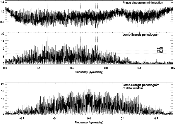
Figure 1: Upper panel: Comparison of the results of phase dispersion minimization and the Lomb-Scargle periodograms based on the observed data from Table 1. Some of the possible solutions, with periods of 3.63293, 3.71058, 4.45633, 5.58098, and 7.94913 days are highlighted. For the Lomb-Scargle periodogram, three levels of the false-alarm probability are indicated. Lower panel: The Lomb-Scargle periodogram of the data window function, with the peak at zero frequency removed. For purpose of clarity, a different frequency domain was used for this panel.

4.1 A 3.7-day period in the radial velocity

The relatively smooth changes in radial velocity within a night prompted us to search for periodic radial velocity changes. We also searched the literature for published radial velocity measurements of RU Lup, and we included data published by Melo (me03 (2003)) in our analysis (see Table 1). Other published velocities of RU Lup lack information on exact times of observation.

The combined dataset we have at our disposal is inhomogeneously sampled in time, sometimes with several observations in short periods of time. The differences between the radial velocities of consecutive spectra is small. Therefore, in order to focus on the long-term evolution of the radial velocity, rather than to contaminate the period analysis with the very short-term variations, we averaged all consecutively observed observations, leaving us with a set of 38 radial velocity measurements, including the 7 values published by Melo. For our analysis we assumed an uncertainty in the radial velocities of $\sigma=\pm 1$ km s^-1.

We analysed the data using two different period-detection methods. These methods are the Lomb-Scargle periodogram (according to the prescription of Horne & Baliunas hb86 (1986)) and phase-dispersion minimization (Stellingwerf pdm (1978)). The resulting diagrams for these methods are shown in Fig. 1.

An important feature of the Lomb-Scargle periodogram is that the height of the peaks in the periodogram allows to make an estimate of the false-alarm probability (FAP). We performed Monte-Carlo simulations to determine the probability that, for a given signal in the periodogram, normally-distributed random fluctuations give rise to a false detection of periodicity (i.e. the FAP). In Fig. 1 we indicate the levels in the periodogram corresponding to a FAP of 0.05, 0.01 and 0.001. The peaks in our periodogram clearly exceed these levels, indicating that there is detectable periodicity in our data, although it is not directly clear which period fits the data best.

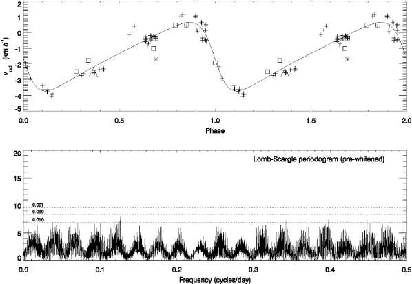
Figure 2: Upper panel: All observations of RU Lup, folded with the 3.71058 day period. Observations marked with $+$ are taken at the VLT, with $*$ at the AAT and $\triangle$ at the CTIO. Observations by Melo (me03 (2003)) are marked with $\square$. Lower panel: The Lomb-Scargle periodogram after pre-whitening of the data with the 3.71058 day period. Levels of the false-alarm probability are indicated.

The difficulty in determining the correct period with the Lomb-Scargle periodogram is for a large part due to the inhomogeneous distribution of our observations in time, producing a broad window function with strong sidelobes. (See Fig. 1). Also, the Lomb-Scargle periodogram relies on the implicit assumption that the signal is purely sinusoidal. Non-sinusoidal signals might be detected, but with lower peaks of significance. Phase-dispersion minimization is unbiased towards the shape of the radial velocity curve, and might detect signals that are difficult to detect with the Lomb-Scargle periodogram.

As can be seen from Fig. 1, the Lomb-Scargle periodogram and Phase-dispersion minimization gave a number of possible solutions. Presented with more than one clear solution, we performed pre-whitening of the radial velocity data and recalculated the periodograms. We found that the pre-whitened periodogram of all periods contained significant levels of power, except for the solution with $P=3.71058$ days. The pre-whitened periodogram for this period is shown in the lower panel of Fig. 2. The remaining power is clearly less than the lowest levels of the FAP. After pre-whitening, we can also estimate the uncertainty in the period (Horne & Baliunas, hb86 (1986)) finding that $P=3.71058\pm 0.0004$ days.

Although this period is well identified by Phase-dispersion minimization, it does not produce a strong peak in the Lomb-Scargle periodogram. However, recalculating the Lomb-Scargle periodogram using calculated radial velocities produced a diagram very similar to the periodogram of the observed data, including peaks of other candidate periods found in the original Lomb-Scargle periodogram This supports our conclusion that the most likely period that fits our data has $P=3.71058$ days.

If the period derived above is identical to the rotational period, this allows us to determine the inclination of RU Lup. Herczeg et al. (herczeg05 (2005)) derived a radius of $1.64$ R_☉ and a mass of $0.65$ M_☉ from the stellar luminosity, and if $P_{\rm rot}\approx 3.71$ days and $v\sin i=9.0\pm 0.9$ km s^-1 (Stempels & Piskunov st02 (2002)) then $i\approx 24\degr$. This is compatible with other observational arguments (Herczeg et al. herczeg05 (2005); Stempels & Piskunov st02 (2002)) that indicate that RU Lup is observed close to pole-on.

4.2 Photometric periodicity?

RU Lup is well-known to exhibit strong erratic photometric variability. Early on, Hoffmeister (hoffmeister65 (1965)) and Plagemann (plagemann (1969)) reported a photometric period of 3.7 days. Giovannelli et al. (giovannelli91 (1991)) found a weak signal corresponding to 3.7 days in the power spectrum when re-analysing the early data, and Drissen et al. (drissen89 (1989)) found some evidence of a 3.7 day period in their linear polarization measurements. However, later analyses including newer data indicated that the 3.7 day photometric period is not significant (Gahm et al. gahm93 (1993); Giovannelli et al. giovannelli94 (1994)).

From 2001 until 2005, RU Lup was also monitored in the $V$-band by the All Sky Automated Survey (ASAS, see Pojmanski asas (2002)). This period of time covers most of our spectroscopic observations of RU Lup. We have analysed the ASAS dataset of RU Lup, obtaining $V=11.23\pm 0.26$, but no periodicity. Neither did we find any short-term correlation between the measured radial velocities in individual observing runs and simultaneous photometric data. We performed several numerical tests on the ASAS data and found that the semi-amplitude of any possible photometric periodicity must be less than 0.12 mag. Periodic variations larger than this would have been detected from these data with high probability.

5 Discussion

Periodic radial velocity changes in photospheric absorption lines may be generated in different ways, and below we will discuss possible sources such as rotational modulation of dark and/or bright spots on the stellar surface, binarity and pulsations.

5.1 Spots

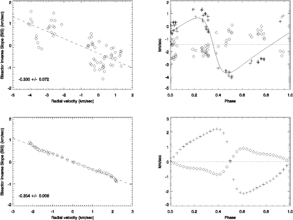
Figure 3: Upper panel — left: The relation between the Bisector Inverse Slope (BIS, see text) and the observed radial velocity of RU Lup. The slope of the best least-squares fit is shown. Upper panel – right: The observed radial velocity ($+$) and the BIS ($\Diamond$) folded with the $3.71058$ day period. The values of the BIS have been plotted with respect to the mean average radial velocity. Lower panel: As in the upper panel, but for a set of synthetic spectra of a star with a photosphere of $T=4000$ K and a spot of $T=3400$ K, a latitude of $60\degr$ and a radius of $35\degr$.

Spots can distort the shape of photospheric line profiles, an effect exploited in Doppler Imaging. Unfortunately, RU Lup has a $v\sin i$ of only 9 km s^-1 making it unsuitable as a target for Doppler Imaging. Still, spots may be an important candidate to consider as a cause of the observed velocity changes in RU Lup.

A critical test of the effects of spots on the stellar line profiles can be performed using line bisector analysis. An inhomogeneous distribution of spots on the stellar surface will make the line profiles appear asymmetric, which is detectable as a change in the line bisector. In addition to changes to the line bisector, spots may cause variations in the apparent radial velocity of the star, within a fraction of its $v\sin i$ value.

Any correlation between the BIS and the apparent radial velocity is often used as a strong indication that the shape of the line profiles changes are due to some process other than genuine shifts in radial velocity. For example, Queloz et al. (queloz01 (2001)) used an anti-correlation between the BIS and the observed radial velocity to show that spots can cause a periodic signal in the apparent radial velocity. Similarly, Santos et al. (santos02 (2002)) used a positive correlation between the BIS and the observed radial velocity to argue that faint light from an undetected companion changes the intrinsic line profile. Dall et al. (dall06 (2006)) also found a positive correlation for EK Eri, and related this to surface activity, or possibly an unseen companion. The absence of a correlation is normally interpreted as a strong argument for genuine changes in radial velocity due to a companion (for example Santos et al. santos03 (2003)).

In the top-left panel of Fig. 3 we show the relation between the BIS and the radial velocity we obtained for RU Lup. As one can see there is an anti-correlation between the BIS and the apparent radial velocity of RU Lup. The anti-correlation is more evident in the top-right panel, where we show both the BIS and the radial velocity as a function of phase.

Although the anti-correlation between the BIS and the radial velocity is a strong indication that surface structures might be responsible for the observed changes in radial velocity, it is important to quantify this effect in terms of spot size and changes in brightness. Therefore, we simulated the effect of starspots on the shape of photospheric lines using a simple model of a spotted star (see Hatzes hatzes02 (2002)).

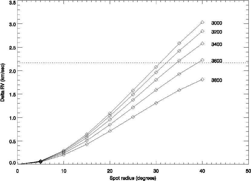
Figure 4: Calculated effect of a stellar spot located at a latitude of 60$\degr$ on the amplitude of radial velocity variations for a range of temperatures and spot radii. The dotted line indicates the observed amplitude of variations in RU Lup.

In this model we assume parameters typical for RU Lup, $T_{\rm eff}$ = 4000 K, $v\sin i$ = 9 km s^-1 and $i=24\degr$. The photosphere was represented by a synthetic K7 V spectrum, while for the spots we used synthetic spectra across a range of temperatures (3000 – 3800 K). The photospheric and spot spectra were then combined to construct disk-integrated synthetic spectra of a spotted star for several rotational phases and spot radii (0 – 40$\degr$). The resulting spectra cover the spectral region 6000 – 6050 Å and have a spectral resolution of about 60 000. For each spectrum we determined the corresponding radial velocity $v_{\rm rad}$, as well as the brightness and the bisector shape through cross-correlation with the spectrum of an unspotted K7 V star.

From our model we find that one single spot at a latitude of $\approx 60\degr$ and on an otherwise undisturbed stellar surface will cause the most dominating effect (i.e. on radial velocity, brightness and line asymmetry). Although using one single spot is the simplest possible model to reflect the observed variations, this does not necessarily reflect the actual distribution. Doppler Imaging of other CTTS has shown that a distribution with several (groups of) spots is more realistic. We therefore interpret the results of our simulation only as a first-order indication of the effect of an asymmetric distribution of spots on the observed line profile.

The shift in observed radial velocity due to a spot is a function of both the spot size and the temperature contrast between the spot and the stellar photosphere, as is illustrated in Fig. 4. This figure shows that, in order to explain the observed amplitude in radial velocity, the surface of RU Lup must have a relatively large spot coverage (similar to a single spot with a radius of $>30\degr$), and that these spots can have (average) surface temperatures in the range 3000 – 3600 K.

We did similar calculations for hot spots, assuming the spot to emit a featureless spectrum (black-body continuum) of 7000 K (Calvet & Gullbring calvet98 (1998)). Because hot spots have a much larger surface brightness than the rest of the photosphere, their contribution to the total spectrum is much stronger than is the case for cool spots. We found that, although asymmetric hot spot may explain changes in radial velocity, the implied spot radius ($\ga 40\degr$) would cause very strong levels of veiling ($\ga 10$), which would correlate strongly with phase. Hot spots would also cause strong phase-related changes in the blue part of the spectrum. We found no evidence for either effect in our observations of RU Lup. In addition, CTTS tend to have typical values of hot spot filling factors around 0.1 – 5% (Calvet & Gullbring calvet98 (1998); Calvet et al. calvet04 (2004)), and not 25 – 50%. Non-polar hot spots also are transient phenomena related to (variable) accretion. We find it therefore unlikely that these short-lived, hot surface features could be responsible for the long-term velocity variations in RU Lup. This, of course, does not rule out active accretion and small hot spots on RU Lup.

Our simulations also allowed us to estimate the magnitude of brightness variations due to spots. Although a cool spot with a radius of $40\degr$ will induce a relatively strong modulation in brightness, it will be difficult to detect this effect from photometry alone, since high levels of veiling will strongly reduce the brightness contrast of such variations. This reduction in brightness contrast between spot and star is also the reason why we were unsuccessful in detecting other spectroscopic signatures of spots, such as molecular bands from TiO.

For each set of simulated spectra we determined the behavior of the BIS, using the same method and template as for the observed spectra. We found that the BIS of the simulated spectra shows an anti-correlation with rotational phase, and that the slope of this correlation depends weakly on both the spot size and temperature. From our set of models, a star with a 35$\degr$ spot of $T=3400$ K shows the best agreement with the observations, fitting the slope of the anti-correlation, as well as the shape and amplitude of the velocity curve. This is illustrated in the lower panels of Fig. 3.

We conclude that it is possible to explain the observed changes in radial velocity in RU Lup with cool spots, and that this requires relatively large surface areas covered with spots. The consistency of the radial velocity variations, which allowed us to establish the rotational period, indicates a long lifetime for the spot structures on RU Lup. Other CTTS for which approximate spot sizes have been determined seem to follow this pattern. Doppler Imaging studies of Sz 68 (Johns-Krull & Hatzes johns97 (1997)), DF Tau (Unruh et al. unruh98 (1998)), SU Aur (Petrov et al. petrov96 (1996); Unruh et al. unruh04 (2004) and MN Lup (Strassmeier et al. strassmeier05 (2005)) all recover large surface areas covered by spots. Modelling of the spot coverage fraction in active stars using molecular band analysis suggests that Doppler Imaging, and thus also bisector analysis, may underestimate the true spot filling factor due to features that do not change the line profile (O’Neal et al. oneil04 (2004)).

The large spot filling factor we find for RU Lup could also be in agreement with the empirical relation between spot filling factor, photospheric temperatures and magnetic field strengths on active dwarfs derived by Berdyugina (berdyugina05 (2006)). This relation would imply a strong magnetic field of the order of 3 kG in this star.

5.2 Binarity

One alternative explanation of the radial velocity variations in RU Lup may be that a low-mass secondary component orbits the star. An elliptic binary orbit with $P=3.71058$ days and $e=0.41$ is compatible with the periodic radial velocity variations observed in RU Lup (see Fig. 2). Both the amplitude and the shape of the velocity curve match the effect of a low-mass secondary orbiting RU Lup.

The mass of the secondary can be determined under the assumption that the axis of rotation are lined up, and that the system rotates synchronously. This is a normal assumption for close binary systems, because the time-scale for synchronization for such systems is relatively small (see Hilditch hilditch (2001) and references therein). The mass function for a single-lined spectroscopic binary is $f(m)={m_{2}^{3}}\sin^{3}i/{(m_{2}+m_{1})^{2}}=1.0361\cdot 10^{-7}\,(1-e^{2})^{3/2}K_{1}^{3}P$, where $e$ is the ellipticity, $K_{1}$ is the amplitude of the velocity variations of the primary in km s^-1, and $P$ the period of the system in days. Using $m_{1}=0.65$ M_☉, $K_{1}=2.17$ km s^-1 and $i=24\degr$, we derive a secondary mass of $m_{2}=0.027$ M_☉, which is well within the brown dwarf regime. The semi-major axis of the primary follows from $a_{1}\sin i=1.9758\cdot 10^{-2}\,(1-e^{2})^{1/2}K_{1}P$ giving $a_{1}=0.36$ R_☉ and $a_{2}=m_{1}/m_{2}\cdot a_{1}=8.5$ R_☉.

Although the orbital solution fits the observed radial velocity of RU Lup, we find the solution of a brown dwarf secondary unlikely. The obtained solution does not allow us to reproduce the observed correlation between the BIS and the radial velocity. While a brown-dwarf binary seems unlikely, our observations cannot dismiss a possible RS CVn-like scenario in which spots and a binary companion cause simultaneous and phased modulation of the radial velocity.

5.3 Pulsations

The loci of fundamental pulsation periods of contracting stars over the HR-diagram were calculated by Gahm & Liseau (gahmlis (1988)). The position of RU Lup in the HR-diagram indicates possible periods on time-scales of hours rather than days (Gahm gahm06 (2006)). Unless there is a not yet identified mode of surface oscillations, it appears that pulsation is not the agent of periodic radial velocity changes.

6 Conclusions

Using standard cross-correlation techniques we have found radial velocity variations in very high resolution spectra of the CTTS RU Lup. The variations span a small range of velocities ($-4$ to $+0.5$ km s^-1) and appear to be periodic ($P\approx 3.71$ days).

These radial velocity variations correlate with the slope of the bisector, indicating that they are probably related to spots on the stellar surface. We quantified this effect by simulating these variations with a model of a spotted star. We find that a large part of the surface of RU Lup has to be covered with long-lived spots of $T\approx 3400$ K to explain the observed changes in the bisector and radial velocity. A large spot coverage indicates that a surface magnetic field of about 3kG can be expected in RU Lup.

We also considered binarity and pulsations as other possible sources of radial velocity variations, but these turned out to be unlikely candidates.

The 3.71 day period in radial velocity we recovered is similar to what was reported in some very early photometric studies of RU Lup. Even though later investigations, including this work, do not confirm any photometric periodicity, it would be of value to repeat multi-colour monitoring, especially in the blue part of the spectrum, to search for underlying weak signals of periodic nature.

- (1) Basri, G., Johns-Krull, C. M., & Mathieu, R. D. 1997, AJ 114, 781
- (2) Berdyugina, S. V., 2005, Living Rev. Solar Phys. 2, 8. URL: http://www.livingreviews.org/lrsp-2005-8
- (3) Calvet, N., & Gullbring, E. 1998, ApJ 509, 802
- (4) Calvet, N., Muzerolle, J., & Brice o, C. 2004, AJ 128, 1294
- (5) Dall, T. H., Santos, N. C., Arentoft, T., Bedding, T. R., & Kjeldsen, H. 2006, A&A 454, 341
- (6) Drissen, L., Bastien, P., & St.-Louis, N., 1989, AJ 97, 814
- (7) Gahm, G. F. 2006, in Proc. Close Binaries in the 21st Century: New Opportunities and Challenges, eds. A. Gimenez, et al., in press
- (8) Gahm G. F., & Liseau, R. 1988, in Proc. Activity in Cool Star Envelopes, eds. O. Havnes, et al., Kluwer Academic Publ., p. 99
- (9) Gahm, G. F., Gullbring, E., Fischerström, C., Lindroos, K. P., Lodén K., 1993, A&AS 100, 371
- (10) Gahm G. F., Petrov, P. P., & Stempels, H. C. 2005, Proc. 13th Cambridge Workshop on Cool Stars, Stellar Systems and the Sun, eds. Favata, F., et al., ESA-SP 560, p. 563
- (11) Giovannelli F. 1994, Space Sci. Rev. 69, 1
- (12) Giovannelli F., Errico, L., Vittone, A. A., & Rossi, C. 1991, A&AS 87, 89
- (13) Guenther, E. W., Lehmann, H., Emerson, J. P., & Staude, J. 1999, A&A 341 768
- (14) Hartmann, L. 1998, Accretion Processes in Star Formation (Cambridge University Press)
- (15) Hatzes, A. P. 2002, Astron. Nachr. 323, 392
- (16) Herczeg, G. J., Walter, F. M., Linsky, J. L., et al. 2005, AJ 129, 2777
- (17) Hilditch, R. W. 2001, An Introduction to Close Binary Stars (Cambridge University Press)
- (18) Hoffmeister, C. 1965, Veröff. Sternwarte Sonneberg 6, 97
- (19) Horne, J. H., & Baliunas, S. L. 1986, ApJ 302, 757
- (20) Johns-Krull, C. M., & Hatzes, A. P. 1997, ApJ 487, 896
- (21) Johns-Krull, C. M., Valenti, J. A., Hatzes, A. P. & Kanaan, A. 1999, ApJ 510, L41
- (22) Joy, A. H. 1945, ApJ 102, 168
- (23) Kurucz, R. L., Furenlid, I., Brault, J., & Testerman, L. 1984, National Solar Observatory Atlas No. 1 (Tucson: NSO)
- (24) Martin, E. L., Magazzù, A., Delfosse, X., & Mathieu, R. D. 2005, A&A 429, 939
- (25) Melo, C. H. F. 2003, A&A 410, 269
- (26) O’Neal, D., Neff, J. E., Saar, S. H., & Cuntz, M. 2004, AJ 128, 1802
- (27) Petrov, P. P., Gullbring, E., Ilyin, I., et al. 1996, A&A 314, 821
- (28) Petrov, P. P., Gahm, G. F., Gameiro, J. F., et al. 2001, A&A, 369, 993
- (29) Piskunov, N. E., & Valenti, J. A. 2002, A&A 385, 1095
- (30) Plagemann, S., 1969, Mem. Soc. Roy. Sci. Liège, 5th series, No 19, p. 331
- (31) Pojmanski, G. 2002, Acta Astronomica, 52, 397
- (32) Queloz, D., Henry, G.W., Sivan, J.P., et al. 2001, A&A 379, 279
- (33) Santos, N.C., Mayor, M., Naef, D., et al. 2002, A&A 392, 215
- (34) Santos, N.C., Udry, S., Mayor, M., et al. 2003, A&A 406, 373
- (35) Stellingwerf, R. F., AJ 224, 953
- (36) Stempels H. C., & Gahm G. F. 2004, A&A 421, 1159
- (37) Stempels H. C., & Piskunov N. 2002, A&A 391, 595
- (38) Stempels H. C., & Piskunov N. 2003, A&A 408, 693
- (39) Strassmeier, K. G., Rice, J. B., Ritter, A., et al. 2005, A&A 440, 1105
- (40) Unruh, Y. C., Collier Cameron, A., & Guenther, E. 1998, MNRAS 295, 781
- (41) Unruh, Y. C., Donati, J.-F., Oliveira, J. M., et al. 2004, MNRAS 348, 1301
- (42) Valenti, J. A. & Johns-Krull, C. M. 2004, Ap&SS 292, 619