A Solution to the Galactic Foreground Problem for LISA

Abstract

Low frequency gravitational wave detectors, such as the Laser Interferometer Space Antenna (LISA), will have to contend with large foregrounds produced by millions of compact galactic binaries in our galaxy. While these galactic signals are interesting in their own right, the unresolved component can obscure other sources. The science yield for the LISA mission can be improved if the brighter and more isolated foreground sources can be identified and regressed from the data. Since the signals overlap with one another we are faced with a “cocktail party” problem of picking out individual conversations in a crowded room. Here we present and implement an end-to-end solution to the galactic foreground problem that is able to resolve tens of thousands of sources from across the LISA band. Our algorithm employs a variant of the Markov Chain Monte Carlo (MCMC) method, which we call the Blocked Annealed Metropolis-Hastings (BAM) algorithm. Following a description of the algorithm and its implementation, we give several examples ranging from searches for a single source to searches for hundreds of overlapping sources. Our examples include data sets from the first round of Mock LISA Data Challenges.

I Introduction

Galactic compact binary systems are expected to be the major source of gravitational waves detected by the LISA observatory lppa . Tens of millions of such binaries will be emitting gravitational waves in the LISA band evans ; lip ; hils ; hils2 ; gils . Though most will be have a signal-to-noise ratio (SNR) too low to be detectable, tens of thousands are expected to be resolvable if optimal signal analysis algorithms are available seth . The signals from unresolved binary systems will constitute a gravitational wave confusion noise. Identification of the brighter galactic binaries will be an important aid to resolving other sources for LISA, such as supermassive black hole binaries (SMBHBs) vech ; lang ; bbw ; rw ; kz and extreme mass ratio inspirals of compact objects into supermassive black holes (EMRIs) cutbar ; emri ; drasco ; drasco_hughes . The SMBHB, EMRI and compact binary signals have small, but non-vanishing overlap with one another, so we will ultimately want a simultaneous fit to all sources and source types.

Various techniques have been proposed to extract the parameters of sources from the LISA data stream. The methods include Markov Chain Monte Carlo Methods MCMC ; MCMC_ed_neil ; vecchio_1 ; vecchio_2 , genetic algorithms genetic , iterative methods gclean ; slicedice , grid-based template searching curt_michele_duncan , tomographic reconstruction browns and time-frequency methods time_freq . For most of these methods (tomography and time-frequency analysis being the exceptions) optimal filtering is accomplished through the construction of templates describing the signals from all sources in the data stream. For LISA, the vast number of sources involved makes a direct approach (such as a grid-based template bank) computationally impractical. It is for this reason ergodic methods such as MCMC and genetic algorithms have been applied to the LISA data analysis problem.

In this work we develop an extension of the MCMC method metro ; haste ; gamer that is able to search the entire LISA band and simultaneously solve for thousands of galactic binaries. Our approach is based on the observation that while some signals can have significant overlap, signals that are well separated in frequency have little or no overlap. We exploit this quasi-locality by breaking the search up into sub-regions in frequency, taking care with edge effects. In a departure from our previous approach MCMC , we do not try and update all the source parameters simultaneously at each iteration. This greatly reduces the computational cost, while still providing a global solution as the full meta-template comprising all the search templates is used to evaluate the likelihood. The parameter updates are now done in small blocks of highly correlated parameters, and the solution is updated using Metropolis-Hastings sampling. Simulated annealing is employed during the search phase to improve the mixing of the chains. We demonstrate this “Blocked Annealed Metropolis-Hastings” (BAM) algorithm on simulated LISA data that contains the signals from monochromatic white dwarf binary systems (WD-WD) immersed in Gaussian instrumental noise.

The paper is organized as follows: In Section II we review the MCMC algorithm and the Metropolis-Hastings sampling kernel. Additionally, we give a description of the BAM algorithm and demonstrate how its computational cost scales with the number of sources being searched for. Section III discusses various aspects of using the BAM algorithm, such as hierarchical searching, optimal choices for search ranges, stopping criteria, and rates of occurrence for false positives and false negatives. Example searches are performed in Section IV, ranging from individual sources to hundreds of sources in a restricted range of the LISA band. Concluding remarks are made in Section V.

II Algorithm Overview

In this section we describe the BAM algorithm and the issues and difficulties that we worked through in the development process. We start with a brief review of the basic MCMC approach and Metropolis-Hastings importance sampling. This is followed by a review of how the extrinsic source parameters are analytically solved for using the F-Statistic. We then describe how the speed of the BAM algorithm scales with the number of sources that are being searched for.

II.1 The Markov Chain Monte Carlo Algorithm and Metropolis-Hastings Sampling

The MCMC algorithm is becoming a familiar tool in gravitational wave data analysis. Initially introduced to the field by Christensen and Meyer cm1 , its application to ground-based interferometers has been explored in the context of parameter extraction of coalescing binaries christ and spinning neutron stars woan . With its ability to explore large parameter spaces while simultaneously performing model selection and noise estimation, the MCMC method is ideally suited to the LISA data analysis problem. The Reverse Jump MCMC algorithm has been applied to the LISA-like problem of identifying a large, yet unknown number of sinusoids in simulated Gaussian noise andrieu ; woan2 . It was shown that the method could correctly identify the number of resolvable signals present in the data and recover the signal parameters and an estimate of the noise level. The MCMC approach was first applied to simulated LISA data in the context of galactic binaries MCMC , and it has since been applied to SMBHBs MCMC_ed_neil ; vecchio_1 ; vecchio_2 .

In using an MCMC approach one wants to generate a sample set, $\{\vec{x}\}$ that corresponds to draws made from the posterior distribution of the system, $p(\vec{\lambda}|s)$. The algorithm to develop such a set is surprisingly simple.

We begin at a point in the parameter space of the binary system(s), $\vec{x}$, (which may or may not be chosen at random) and propose a jump to a new position, $\vec{y}$, based on some proposal distribution, $q(\cdot|\vec{x})$. The Hastings ratio is calculated using,

$$H=\frac{p(\vec{y})p(s|\vec{y})q(\vec{x}|\vec{y})}{p(\vec{x})p(s|\vec{x})q(\vec{y}|\vec{x})}\,,$$ (1)

where $p(\vec{x})$ is the prior of the parameters at $\vec{x}$, $q(\vec{x}|\vec{y})$ is the value of the proposal distribution for a jump from $\vec{x}$ to $\vec{y}$, and $p(s|\vec{x})$ is the likelihood at $\vec{x}$. The likelihood function, if the noise is a normal process with zero mean, is given by sam

$$p(s|\vec{x})=C\exp\left[-\frac{1}{2}\left((s-h(\vec{x}))|(s-h(\vec{x}))\right)\right]\,,$$ (2)

where the normalization constant $C$ is independent of the signal, $s$, and $(a|b)$ denotes the noise weighted inner product

$$(a|b)=2\int_{0}^{\infty}\frac{\tilde{a}^{\ast}(f)\tilde{b}(f)+\tilde{a}(f)\tilde{b}^{\ast}(f)}{S_{n}(f)}\,df,$$ (3)

where $a$ and $b$ are the gravitational waveforms, and $S_{n}(f)$ is the one-sided noise spectral density. The jump will be accepted with probability $\alpha={\rm min}(1,H)$. If the jump is rejected (Metropolis rejection metro ) the chain remains at its current state, $\vec{x}$. Repeated jumps will produce a Markov chain whose stationary distribution is equal to the posterior distribution in question, $p(\vec{x}|s)$. Andrieu et al mcmc_hist ; andrieu provide a more general and thorough review of MCMC methods.

The convergence to the correct posterior will occur for any (non-trivial) proposal distribution gilks . However, the more accurate the proposal distribution is at modeling the posterior distribution the quicker the chain will convergence. Since we do not know the form of the posterior in advance of running the chain, we instead opt for maximum flexibility in our choice of proposal distribution. We accomplish this by using a mixture of proposal distributions, including occasional “bold” proposals that attempt large changes in the parameter values along with many “timid” proposals that attempt small changes in the parameter values of the chain (for a detailed description of some of these proposals see MCMC ). Also added to our list of proposals are a few “tailored” proposals. These are proposed jumps based on our knowledge of the symmetries and degeneracies of the likelihood surface. For example, for LISA there is a secondary maxima in the likelihood surface of a binary system that corresponds to a reflection about the ecliptic equator combined with a shift of $\pi$ in the ecliptic longitude. Thus, we include a proposal that attempts such a reflection.

Another tailored proposal that was highly effective uses the fact that local maxima occur in the likelihood surface at multiples of the modulation frequency ($f_{m}=1/{\rm year}$). The presence of these maxima are easily understood. The detector response imparts sidebands on the monochromatic Barycenter signal to produce a comb whose teeth are spaced by the modulation frequency. A template with a Barycenter frequency offset from the signal by a multiple of $f_{m}$ will produce a similar comb whose teeth align with those of the signal. The fit can be improved by adjusting the other template parameters to better match the shape of the source comb. Figure 1 shows the power spectrum of a source and a template offset by $1f_{m}$ in frequency, while in Figure 2 the template has had its other parameters altered to better fit the source comb. This improves the log likelihood from $16.7\%$ to $66.4\%$ of the true parameter value. It proved to be difficult to find an analytic description of how the other parameters should be modified to improve the fit, so we went with a simple proposal that shifted the frequency of the source by $1f_{m}+\epsilon$, and shifted the other parameters using a uniform draw in a small range around the current binary parameters.

Since the search used an F-statistic to extremize over the amplitude, inclination angle, polarization angle and initial phase, we only needed to assign priors to the frequency and sky location. For the frequency we used a uniform prior across the search range, and for the sky locations we used a distance weighted galactic distribution.

Figure 1: Spectrum of a source and template with the same parameters save their frequencies, which differ by one modulation frequency. The source has $f=3.0{\rm mHz}$, $A=1.4\times 10^{-22}$, $\theta=1.0$, $\phi=3.14159$, $\psi=0.5$, $\iota=0.785398$, and $\varphi_{o}=0.0$.

Figure 2: Spectrum of a sources and a template with frequencies that differ by one modulation frequency. The parameters of the template have been adjusted to maximize the overlap. The source has the same parameters as in Figure 1, while the template has $A=1.47254\times 10^{-22}$, $f=3.000031688{\rm mHz}$, $\theta=0.787087$, $\phi=3.18781$, $\psi=0.51218$, $\iota=0.89419$, and $\varphi_{o}=0.179034$.

While a general MCMC algorithm functions as both a means to search the likelihood surface and sample from the posterior distribution, the Markovian nature is only required for the sampling portion of the process. If one is able to find the neighborhood of the true parameters by other means, and then implements an MCMC algorithm from that point, the subsequent samples will recover the correct posterior distribution. It is with this in mind that we chose to relax the requirement that all of our proposal distributions be Markovian. The algorithm described above remains the same, but is now open to non-Markovian proposal distributions. We refer to this non-MCMC approach as Metropolis-Hastings importance sampling. One example of a non-Markovian proposal involves how we implement the previously described $1f_{m}$ jump. Early in the search phase, if one of these proposals was accepted, a second (identical) jump was attempted. The reason for this is that just as a local maximum occurs $\sim 1f_{m}$ away from the global maximum, another (smaller) local maximum occurs $\sim 2f_{m}$ away. In fact, a chain of maxima occur spaced about one modulation frequency apart from each other in likelihood space (see Figure 3). This non-Markovian move allowed searchers to “island-hop” around the likelihood surface if it found itself on one of the maxima in the island chain.

For the purpose of searching to determine the neighborhood of the true parameters, which is the focus of this work, we allow ourselves the extra freedom provided by non-Markovian Metropolis-Hastings importance sampling and simulated annealing (described below). Once the search phase is complete the non-Markovian moves are suspended, and the algorithm performs a standard MCMC exploration of the posterior distribution.

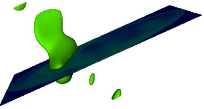
Figure 3: Contours of constant likelihood for a single, monochromatic WD-WD binary system. Sky position directions lie in the plane shown, while frequency is directed orthogonal to the plane. The visible maxima are separated by approximately one modulation frequency.

To encourage the chains to explore the full parameter space and to discourage the chains from getting stuck a local maxima we employ simulated annealing during the search phase. This is done by multiplying the noise-weighted inner product by an “inverse temperature” $\beta$, and applying the cooling schedule

$$\beta=\left\{\begin{tabular}[]{ll}$\beta_{0}\left(\frac{1}{\beta_{0}}\right)^{i/N_{c}}$&$0\leq i\leq N_{c}$\\ 1&$i>N_{c}$\end{tabular}.\right.$$ (4)

Here $\beta_{0}$ is the initial heating factor and $N_{c}$ is the length of the annealing phase. The choice of $\beta_{0}$ depends on the SNR of the sources. When very bright sources are present we set $\beta_{0}\sim 10^{-3}$, while smaller values of $\beta_{0}\sim 10^{-2}$ work better once the brightest sources have been removed. Our criteria for choosing $\beta_{0}$ was that the chains should explore the full parameter range during the first 1000 or so iterations. If full range movement was not seen we dialed up the heat. The choice of $N_{c}$ depends on $\beta_{0}$, and can be set by demanding that it takes, say, 500 steps for $\beta$ to decrease by a factor of two.

II.2 F-Statistic

The F-statistic fstat uses multiple linear filters to obtain the extremum for the likelihood over the extrinsic parameters of the signal. Using the F-statistic one can search the intrinsic parameters, and recover the extrinsic parameters as a last step in the process. For a monochromatic binary detected by LISA, this reduces the search space to three parameters: frequency and sky location ($\theta$, $\phi$). Note: the tumbling orbit of LISA induces modulations of the frequency into the signal, thus creating and interdependency in the signal between frequency and sky location that prevents $\theta$ and $\phi$ from being treated as purely extrinsic quantities.

At low-frequencies in the LISA response to a gravitational wave can be written:

$$h(t)=h_{+}(t)F^{+}(t)+h_{\times}(t)F^{\times}(t)\,,$$ (5)

where $h_{+}(t)$ and $h_{\times}(t)$ are the two polarizations of the incident gravitational wave cc ; cr , which for a monochromatic binary, to leading post-Newtonian order, are given by:

$$h_{+}(t) = A(1+\cos^{2}\iota)\cos(\Phi(t)+\varphi_{0})$$

$$h_{\times}(t) = -2A\cos\iota\,\sin(\Phi(t)+\varphi_{0}).$$ (6)

$F^{+}(t)$ and $F^{\times}(t)$ are the beam pattern factors:

$$F^{+}(t) = \frac{1}{2}\left(\cos 2\psi\,D^{+}(t)-\sin 2\psi\,D^{\times}(t)\right)$$

$$F^{\times}(t) = \frac{1}{2}\left(\sin 2\psi\,D^{+}(t)+\cos 2\psi\,D^{\times}(t)\right)$$ (7)

where $D^{+}(t)$ and $D^{\times}(t)$ are the detector pattern functions, whose mathematical form can be found in equations (36) and (37) of Ref.rigad .

In the gravitational wave phase

$$\Phi(t;f,\theta,\phi)=2\pi ft+2\pi f{\rm AU}\sin\theta\cos(2\pi f_{m}t-\phi),$$ (8)

one can see the coupling of the sky location and the frequency through the term that depends on the radius of LISA’s orbit, 1 AU, and its orbital modulation frequency, $f_{m}=1/{\rm year}$. For the low frequency galactic sources we are considering, the gravitational wave amplitude, $A$, is effectively constant. Thus (5) can be rearranged as:

$$h(t)=\sum_{i=1}^{4}a_{i}(A,\psi,\iota,\varphi_{0})A^{i}(t;f,\theta,\phi)\,,$$ (9)

where the time-independent amplitudes $a_{i}$ are given by

$$a_{1} = \frac{A}{2}\left((1+\cos^{2}\iota)\cos\varphi_{0}\cos 2\psi-2\cos\iota\sin\varphi_{0}\sin 2\psi\right),$$

$$a_{2} = -\frac{A}{2}\left(2\cos\iota\sin\varphi_{0}\cos 2\psi+(1+\cos^{2}\iota)\cos\varphi_{0}\sin 2\psi\right),$$

$$a_{3} = -\frac{A}{2}\left(2\cos\iota\cos\varphi_{0}\sin 2\psi+(1+\cos^{2}\iota)\sin\varphi_{0}\cos 2\psi\right),$$

$$a_{4} = \frac{A}{2}\left((1+\cos^{2}\iota)\sin\varphi_{0}\sin 2\psi-2\cos\iota\cos\varphi_{0}\cos 2\psi\right),$$

and the time-dependent functions $A^{i}(t)$ are given by

$$A^{1}(t) = D^{+}(t;\theta,\phi)\cos\Phi(t;f,\theta,\phi)$$

$$A^{2}(t) = D^{\times}(t;\theta,\phi)\cos\Phi(t;f,\theta,\phi)$$

$$A^{3}(t) = D^{+}(t;\theta,\phi)\sin\Phi(t;f,\theta,\phi)$$

$$A^{4}(t) = D^{\times}(t;\theta,\phi)\sin\Phi(t;f,\theta,\phi)\,.$$ (11)

Writing LISA’s signal as a superposition of gravitational waves and noise,

$$s_{\alpha}(t)=h_{\alpha}(t,\vec{\lambda})+n_{\alpha}(t)=\sum_{i=1}^{N}h^{i}_{\alpha}(t,\vec{\lambda}_{i})+n_{\alpha}(t)\,,$$ (12)

and defining the four constants $N^{i}=(s|A^{i})$ and the $M$-matrix, $M^{ij}=(A^{i}|A^{j})$, one can express (9) as a matrix equation:

$$M_{ij}a^{j}=N_{i}\,.$$ (13)

Therefore, with a signal from LISA and the three intrinsic parameter values, one can solve (by iteration or inversion) for the the amplitudes, and thus the extrinsic parameters. The values of the intrinsic parameters are found by use of iterative Metropolis-Hastings importance sampling. The extrinsic parameter values are given by:

$$A = \frac{A_{+}+\sqrt{A_{+}^{2}-A_{\times}^{2}}}{2}$$

$$\psi = \frac{1}{2}\arctan\left(\frac{A_{+}a_{4}-A_{\times}a_{1}}{-(A_{\times}a_{2}+A_{+}a_{3})}\right)$$

$$\iota = \arccos\left(\frac{-A_{\times}}{A_{+}+\sqrt{A_{+}^{2}-A_{\times}^{2}}}\right)$$

$$\varphi_{0} = \arctan\left(\frac{c(A_{+}a_{4}-A_{\times}a_{1})}{-c(A_{\times}a_{3}+A_{+}a_{2})}\right)$$ (14)

where

$$A_{+} = \sqrt{(a_{1}+a_{4})^{2}+(a_{2}-a_{3})^{2}}$$

$$+\sqrt{(a_{1}-a_{4})^{2}+(a_{2}+a_{3})^{2}}$$

$$A_{\times} = \sqrt{(a_{1}+a_{4})^{2}+(a_{2}-a_{3})^{2}}$$

$$-\sqrt{(a_{1}-a_{4})^{2}+(a_{2}+a_{3})^{2}}$$

$$c = {\rm sign}(\sin(2\psi))\,.$$ (15)

This description of the F-statistic automatically incorporates the two independent LISA channels through the use of the dual-channel noise weighted inner product:

We generalize the F-statistic to handle $N$ overlapping sources by writing $i=4K+l$, where $K$ labels the source and $l=1\rightarrow 4$ labels the four filters for each source. The F-statistic has the same form, but with $4N$ linear filters $N^{i}$, and $M^{ij}$ is a $4N\times 4N$ dimensional matrix. For slowly evolving galactic binaries, which dominate the confusion problem, the limited bandwidth of each individual signal means that the $M^{ij}$ is band diagonal, which lessens the difficulty in solving (13) for the large numbers of sources that are expected to be detected.

II.3 The Blocked Annealed Metropolis-Hastings Algorithm

A Gibbs Sampler gemans is a special case of the Metropolis-Hastings algorithm described above in which each parameter, in the set of all parameters, is updated sequentially using a proposal distribution that is the conditional of the posterior evaluated at the current values of the other parameters. The mixing rate can be improved by simultaneously updating blocks of highly correlated parameters, to give what is know as the Blocked-Gibbs algorithm jensen . Since it can be difficult to evaluate the full conditionals required for Gibbs sampling, we decided to stick to Metropolis-Hastings sampling.

The blocks in the BAM algorithm are small sub-units of the frequency range being searched. As can be seen in Figure 4, which shows a schematic representation of a search region in our BAM algorithm, the search region is broken up into equal sized blocks. The algorithm steps through these blocks sequentially, updating all sources within a given block simultaneously. After all blocks have been updated, they are shifted by one-half the width of a block for the next round of updates. This allows two correlated sources that might happen to be located on opposite sides of a border between two neighboring blocks to be updated together on every other update. This blocking provides a means to handle highly correlated searchers/sources, and provides an even greater benefit which is covered in  II.4.

Figure 4: A schematic representation of a search region in frequency space, showing the block structure of some the BAM algorithm.

This simple extension to an MCMC algorithm allowed for quick and robust searching of isolated data snippets with up to $\sim 100$ templates (the limit on the number of templates is due to the computational cost of the multi-source F-statistic). In order to be able to handle the entire LISA band, we have to break the search up into sub-regions containing a manageable number of sources. This introduced the problem of edge effects from sources whose frequency lay just outside the chosen search region, but deposited power into the search region. To combat the edge effects we introduced “wings” and an “acceptance window.” The purpose of the wings is to create a buffer between the chosen search region and the regions beyond, so that sources in those outer regions would not adversely affect the searchers in the acceptance window. The search would be run the same as before, but at the end only those searchers inside the acceptance window would be considered as having been found. Searchers that ended up in the wings were discarded (even though many might be perfectly good fits to actual sources). This would allow us step through frequency space, using multiple search regions. But that was not enough.

A problem, which we call “slamming,” can occur when a bright source lies just outside the range of the chosen search region. Slamming is the tendency of the searchers to migrate to the edge of the search region as the searchers try to fit to the portion of the power from the source outside the search region which is bleeding into the search region. Since the search region contains only a portion of the signal from that particular source, a single searcher is a poor match, and so other searchers soon are recruited to fix-up the fit. Figure 5 shows a case of slamming, where four searchers (in a data snippet with four sources) are drawn off to the edge of the search region by a bright source just outside the search region. A tell-tale feature of slamming is the large amplitudes of the searchers and their high degree of correlation or anti-correlation.

One fix to the slamming problem is to weight the matches in the wings less than matches in the acceptance window. We do this by attenuating the contribution from the wings in the noise weighted inner product. The attenuation is done by increasing the noise spectral density in the wings, which we call “wing noise.” We exponentially increase the noise spectral density, starting at the edge of the acceptance window, as shown in Figure 4. This addition to the algorithm is quite effective at lessening the impact on the likelihood of a searcher fitting power bleeding into wings of the search region. Figure 6 shows a search using wing noise in the same region as Figure 5. As can be seen there is no slamming, and the searchers were able to find the true sources.

Another fix to the slamming problem is to use information about bright sources that lay outside the search region, but close enough that their signals overlap with the search region, in the search process (e.g. subtracting the signal of such sources from the data snippet). This requires knowledge of the bright sources, but such knowledge can be gained by performing initial, exploratory searches for a few sources in the area surrounding the search region in question. As one is free to choose the number of searchers and the ranges of the search, one can use the BAM algorithm hierarchically, if desired, to seek out the brightest sources in a pilot search of the data. Information gleaned from the pilot searches can then be used to subtract bright sources that might lead to slamming. This hierarchical approach will be described in more detail in the Section III.1. In general use of our BAM algorithm, we use both wing noise and information about bright sources outside the search regions to lessen the chance of slamming.

Figure 5: An example of slamming, in which four searchers are drawn to the edge of the search region by a bright source placed just outside the search region.

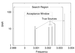
Figure 6: The same search shown in Figure 5, but with the inclusion of wing noise. The wing noise has cured the slamming.

II.4 Time Scaling

Since there are expected to be $15,000^{+}$ resolvable galactic binary systems in the LISA data, we need to be sure that any algorithm developed will be able to search for such a large number of sources in a practical period of time. A pure BAM algorithm that employed a meta template that is the sum of templates from individual sources and simple proposal updates would have a computational cost that scaled linearly in the the number of sources since the cost per source would be constant. The goal of a purely linear scaling is unrealizable in the current version of the BAM algorithm for two reasons.

First, in using the F-statistic to calculate the likelihood values we are required to solve equation (13) for the time-independent amplitudes $a_{i}$. Inverting this equation would scale as $N^{3}$, and while solving for the amplitudes using an iterative method is significantly better it does not scale linearly with $N$. The next update to the algorithm will be to discontinue use of the F-statistic and return to a seven parameter (per binary system) search.

The second impediment is that some proposal distributions, such as a multivariate normal distribution jumping along the eigendirections of the variance-covariance matrix are inherently non-linear in computational cost (calculation of the Fisher Information Matrix alone scales as $N^{2}$). It is here that the use of the blocks shows great benefit. Figure 7 shows how the time to perform a searcher update is affected by the number of searchers. The plot shows the average cost per individual searcher that is updated in a search using only multivariate normal proposal distributions. In one case, all searchers are updated simultaneously (i.e. the entire search region is treated as one block). In the other case, breaking the updates into the blocks lessens the number of searchers being updated simultaneously, greatly reducing the overall computational cost as the number of sources grows. The search was performed on a one year data stream in a $0.01{\rm mHz}$ snippet starting at frequency of $3{\rm mHz}$ with blocks that were $4/year$ wide. Up through $N=20$, no blocks contained more than one search template and the increase in computational cost per search template update was just $1.25$ times greater than a single template search, due solely to the use of the multi-source F-statistic. Beyond $N=20$ the blocks began to contain more than one searcher, and the non-linear nature of the normal proposal started to drive up the cost per update.

Figure 7: Plot of the average computational time per update per search template for two cases, one where all sources are updated simultaneously, and the other where block updates are used. The computational time (y-axis) has been scaled by the average time per update for a single source search. The increase in cost per template update grows much more slowly for the blocked search. To achieve linear scaling in the total cost of the BAM algorithm we would need a constant computational cost per individual template update.

III Issues when Using the Algorithm

Thus far we have described the features of the BAM algorithm, and discussed how those features aid in optimizing the algorithm. In this section some of the implementation issues will be addressed. We will discuss choices of the sizes of search regions, the sizes of the wings, hierarchical searching, stopping criteria, and false-positive/false-negative levels.

III.1 Hierarchical Method

We are able to perform searches in a hierarchical manner simply by choosing to use less search templates than their are sources. For example, if we search a region that contains $10$ sources with a meta-template built from $2$ galactic binary templates, the algorithm will generally recover the $2$ sources that return the highest likelihood value (usually they will correspond to the highest SNR sources in the region). In this hierarchical approach the solution for the brightest sources will be thrown off by the sources that were neglected, but this bias can be corrected at subsequent stages in the hierarchy. At the next stage in the hierarchy more galactic binary templates are used, with the information from the earlier searches providing starting locations for some of the search templates.

Figure 8 describes an example where a $1000f_{m}$ data snippet containing $281$ sources with a observation time of one year was searched using $10$, $30$, and $50$ searchers. In the case using $10$ searchers, the $10$ sources with the highest SNRs were found, while for the case with $30$ searchers only $25$ of the $30$ highest SNR sources were among those found (the other $5$ searchers did find true sources, albeit with lower SNRs).

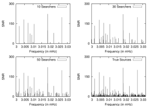
Figure 8: Plot of the recovered (and true) parameter frequencies and their respective SNRs for the sources recovered by the BAM algorithm searching a $1000f_{m}$ data snippet containing $281$ sources with a $1$ year time of observation using $10$, $30$, and $50$ searchers.

One may be tempted to subtract the signals of sources found in the pilot search, before looking for more sources in the region, but our experience leads us to believe that this is not the best way to proceed. In a hierarchical search the initial solution for the bright sources will be thrown off by dimmer sources that they overlap with. To stop these errors from propagating it is better to allow the algorithm to refine the fit to the bright sources at subsequent stages in the hierarchy.

Instead of removing the signal from the data stream, we include the information in the meta-template represented by the combination of the search templates. Within the framework of our algorithm one has several options of how to include the information at subsequent stages. One option is to begin the next search with some of the search templates at the source locations determined at the previous iteration, then allowing them to behave like any other searchers from that point on. Another option is to hold the intrinsic parameters of the previously determined signals fixed during the high heat portion of the annealing phase (the extrinsic parameters of all templates are still updated since we are using a multi-template F-Statistic). The advantage of the later approach is that it protects the information gleaned from earlier stages in the hierarchy, as there is a danger that a previously determined template will be dislodged during the annealing phase. When the temperature reaches a selected value, the constraints are withdrawn and the inherited search templates get treated like any other. This allows the information gathered in the earlier runs to be preserved, and also allows for adjustments to be made to the parameters as needed due to the inclusion of other searchers.

Another benefit is that such hierarchical searching can be used to improve efficiency. Knowing where the very bright sources are in the data snippet can be used to lessen the sizes of the wings of the search regions. This will be discussed in more detail in the next subsection.

III.2 Choosing Window Sizes

There are several factors that influence the choice of window size. In Subsection II.4 we saw that the cost per template update grows with the number of templates in a window. This argues for using small search windows. However, in Subsection II.3 we saw that it was necessary to include a wing region to mitigate edge effects, and any signals recovered in the wings had to be discarded. Thus, we would like for the wings to cover a small fraction of the search window, so that the fraction of templates assigned to wings is small. The size of the wings is determined by the typical bandwidth of a source. A natural choice is to set the wing size equal to the typical half-bandwidth as this ensures that little power leaks into the acceptance window. The source bandwidth is determined by two factors, the width of the sideband comb:

$$B_{c}\approx 2\left(5+2\pi f\frac{1{\rm AU}}{c}\right)f_{m}$$ (16)

and the degree of spectral leakage caused by the finite observation time. The spectral leakage depends on the amount the carrier frequency differs from being an integer multiple of $1/T_{\rm obs}$, and falls off inversely with the number of frequency bins. For observation times on the order of years and for frequencies in the milli-Hertz range, the two contributions to the bandwidth are of similar size. Somewhat larger wings are needed if very bright sources have not been regressed from neighboring frequency windows.

These physical considerations dictate a total wing size of $\sim 15\rightarrow 30f_{m}$, and we would like to use snippets considerably larger than this in order to maximize the fraction of the templates that appear in the acceptance window. The problem with this is that in regions of high source density we end up with template densities of 1 per $\sim 4$ frequency bins, so for a 1 year data stream the wings alone account for $4\rightarrow 7$ templates. Thus, to keep us in the regime where the cost per update is close to that of a single source, we were forced to use snippets where the acceptance window was comparable in size to the wings. In future upgrades we hope to improve the scaling of the algorithm so that we can use larger search windows.

III.3 Stopping Criteria

In LISA data analysis we will not only have to determine source parameters, but also the number of sources that can be resolved. Studies of the galactic confusion noise levels hils ; hils2 ; gils ; sterl ; seth ; bc provide some answers concerning source populations across the LISA band, as well as estimates of the number of resolvable binaries as a function of frequency seth . However, this information is better suited to determining the number of source templates to start with, than the number with which to end. In order to discover where we must stop we will have to listen to the data.

Models with more parameters will always produce better fits to the data, but beyond a certain point the recovered parameters become meaningless. What we seek is the best fit to the data with the simplest possible model. For a model with uniform priors we seek to minimize

$$\chi^{2}=(s-h|s-h)\,,$$ (17)

using the smallest number of source templates. Using Fisher matrix techniques it can be shown that the expectation value of this quantity is given by

$$\langle\chi^{2}\rangle={\cal N}-D\,,$$ (18)

where ${\cal N}$ is the total number of data points and $D$ is the model dimension. As one might have anticipated, it does not make sense to use a model with more parameters than there are data points. This sets an upper limit of 1 source template every $\sim 2$ frequency bins, as there are 4 data points per frequency bin (2 independent data channels, each with a real and imaginary part), and 7 parameters per template. More refined criteria, such as the Bayesian evidence, set more stringent stopping criteria.

There have been many different suggestions of how to weight goodness of fit against model complexity. Two in common use are the Akaike Information Critera (AIC) and the Bayesian Information Criteria (BIC) schwarz . We tried both, and found neither to be particularly satisfactory, settling instead on the Laplace approximation to the full Bayesian evidence. The evidence $p_{X}(s)$ for a model $X$ given data $s$ is given by the integral

$$p_{X}(s)=\int p(s|\vec{\lambda},X)p(\vec{\lambda},X)d\vec{\lambda}\,.$$ (19)

Computing this integral is extremely expensive for high dimension models, but the Laplace approximation provides the estimate:

$$p_{X}(s)\simeq p(s|\vec{\lambda}_{\rm ML},X)\left(\frac{\Delta V_{X}}{V_{X}}\right)\,,$$ (20)

where $p(s|\vec{\lambda}_{\rm ML},X)$ is the maximum likelihood for the model, $V_{X}$ is the volume of the model’s parameter space, and $\Delta V_{X}$ is the volume of the uncertainty ellipsoid (which we estimate using a Fisher Information Matrix). In general, adding another source template to the model will increase the likelihood, however, the $\Delta V_{X}/V_{X}$ term penalizes larger models and serves as a built in Occam factor.

As an example we will look at a data snippet containing $4$ sources. The source parameters and SNRs are shown in Table 1. There is one dim source which is not expected to be recovered (see Section III.4 for more details). Figure 9 plots the logarithms of the evidence and likelihood for models of increasing size. One can see that the evidence is peaked at the model with 3 source templates, while the likelihood continues to climb as the model dimension is increased. This tells us that the data favors a model with $3$ sources over one with $4$.

Table 1: Source Parameter for the $4$ sources in the data snippet

SNR	$A$ ($10^{-24}$)	$f$ (mHz)	$\theta$	$\phi$	$\psi$	$\iota$	$\varphi_{0}$
1.23	2.05	3.001514406	1.259	4.012	0.759	1.183	2.551
7.67	10.8	3.000315843	2.437	2.753	2.484	2.173	2.550
9.65	12.1	3.000454748	2.198	0.422	2.880	2.263	2.991
10.76	9.27	3.001985584	1.336	5.863	0.931	2.805	4.048

Figure 9: Plot of the magnitude of the logarithms of the likelihood and evidence for increasing numbers of searchers, searching a data snippet with sources whose parameters are listed in Table 1 injected into it.

An alternative approach to model selection is to use the Reverse Jump MCMC algorithm, which allows for transitions between models of different dimension. The fraction of the time the chain spends exploring each model is used as a measure of the relative evidence for the different models. We plan to use the RJMCMC approach in future versions of the algorithm.

One limitation of the way we have formulated our Bayesian model selection is that the evidence for a zero source model is ill defined, so we cannot compare models with 0 and 1 source templates. This limitation can be removed if we expand our models to include the instrument noise parameters, which we plan to do in future versions of the algorithm.

For those that favor the Frequentist approach to data analysis we provide some rough estimates of the false alarm and false dismissal rates in the following subsections.

III.4 False Negatives

Here we study the detection rate for the BAM algorithm as a function of the SNR of an isolated source. To this end we performed searches of data snippets between $3{\rm mHz}$ and $3.031688{\rm mHz}$ (a $1000f_{m}$ segment of the LISA band), each containing a single source. A set of parameters for $100$ sources were chosen at random. Keeping all other parameters constant, the amplitudes were varied to increase the SNR. Simulated data sets for each of the 100 sources were created at different SNR levels. The BAM algorithm was then applied to the simulated data using short chains of $15,000$ steps ($10,000$ steps in the annealing phase and $5,000$ set in the sampling phase of each run). The searches were also run using longer chains, consisting of $75,000$ steps ($50,000$ annealing/$25,000$ sampling). For each of two types of chains two analysis methods were used to determined the parameter values. In one method the parameter values were determined by using average values of the parameters in the chain from the sampling phase (i.e. Bayes estimates). In the second method the parameter values were determined from the mode of the parameter histograms from the sampling phase (i.e. MAP estimates). Figure 10 shows the detection probabilities for these searches based on the two analysis methods. The resulting parameter set is called a detection when they deviate by less than $5-\sigma$ in each of the true source’s intrinsic parameters (for more discussion on this cut-off see Section IV).

As expected, the detection probability depends on the length of the chain, with the longer chains giving higher detection rates. However, a single very long chain is not the best way to ensure detection. Consider the search for sources with ${\rm SNR}=5$ using the MAP parameter estimates. The detection rate for the shorter chains were $0.45$, while for the the longer chain the rate was $0.57$. However, if the search for a single ${\rm SNR}=5$ source is repeated multiple times, the detection rate also comes out at $\sim 0.45$. Thus, if the short chain search is run twice and the results from the two runs are combined, the detection probability improves to $\sim 1-0.55^{2}=0.7$, at a total cost of 30,000 steps, which is still less than half the cost of the long chain searches.

Figure 10: Probability of detection of a source using the BAM algorithm as a function of source SNR.

Of the two methods for determining the source parameters, the MAP performed better than the Bayes estimate in the low SNR region. On the other hand, the MAP is harder to compute, especially when there are a large number of sources, so the current implementation of the full scale BAM algorithm still uses Bayes estimates. This will be corrected in future versions.

III.5 False Positives

We now turn our attention to computing the false alarm rate by searching data streams that contain only instrument noise. We employed two approaches: in the first we perform multiple searches with differing noise realizations and in the second we performed an extended search of one noise realization.

For the first test we performed $20,000$ searches using a single search template in the same frequency band we used to study the false negatives. Figure 11 shows a histogram of the SNRs for the finishing points of the searches. This can be used to give an idea as to the level where false positive begin to become a concern. In this frequency range, the histogram tells us that more than $99\%$ of the searches ended on parameters leading to a SNR less than $5$. So in accepting any result from a search with SNR above $5$ in this regime there is roughly a $1\%$ chance of accepting a false positive, with the probability dropping precipitously for searchers returning higher SNRs. We repeated the analysis at different frequencies and found the false positive level to be much the same across the LISA frequency band.

Figure 11: Histogram of the SNRs for searches on source-free noise in a $100f_{m}$ band starting at $3{\rm mHz}$.

The second test used the same $1000f_{m}$ band at $3{\rm mHz}$, but now a single long chain of one million steps was performed. Figure 12 shows the frequency parameter over $100,000$ steps in the chain. One notices that the chain does not lock in on any particular frequency, rather it continually wanders about the entire search region. While this is common, it is not always the case, as instrument noise can sometimes mimic a monochromatic source well enough to slow or even stop such exploratory movement in a chain. Two other reliable indicators of a false positive are the amplitude and the inclination angle of the binary system. Figures 13 and 14 show their respective histograms. The cosine of the inclination angle is peaked around zero, and the amplitude is peaked at a level that gives templates whose spectral density has the same magnitude as the noise. The reason for these preferences is that they allow the template to optimally match the noise in the two LISA data channels. An inclination angle of $\pi/2$ gives equal weight to the two channels, which allows the template to match the noise level in both channels equally well.

Figure 12: Plot of the frequency steps in a chain searching source-free noise in a $1000f_{m}$ band starting at $3{\rm mHz}$.

Figure 13: Histogram of the cosine of the inclination angle for a chain searching source-free noise in a $1000f_{m}$ band starting at $3{\rm mHz}$.

Figure 14: Histogram of the amplitude parameter for a chain searching source-free noise in a $1000f_{m}$ band starting at $3{\rm mHz}$.

To summarize, if the BAM algorithm recovers a source with ${\rm SNR}\geq 5$ it is unlikely to be a false positive. Moreover, the chains show some very characteristic features when the templates are just matching noise, and these features can be used as a diagnostic to exclude false positives. Lastly, one can always run the search multiple times, and if the same same set of parameters are recovered over and over again it is less likely that we have found a false positive.

IV Example Searches

In this section we show the results of several types of searches performed with the BAM algorithm. While results for single source searches are easy to describe, when the search is for hundreds of sources, and there are hundreds of successes, the numbers are much harder to present in a condensed manner. To that end, we will present multiple search cases using plots like those in Figure 8, where the frequency values are shown, and we will list the deviations of the recovered intrinsic parameters scaled by the uncertainties given by the Fisher Information Matrix for the sources. Since we are mostly interested in the search phase of the algorithm the post-search MCMC runs we chosen to be rather short, so the recovered posteriors are a little ragged. With this in mind we set our cut-off criteria for “finding” a source at a deviation of $5-\sigma$ from any one of the true source’s intrinsic parameters. In practice this cut-off was fairly robust as any template that did not have all parameters within a few $\sigma$ of the source typically had one or more parameters that were tens to hundreds of $\sigma$ out. We also imposed was a SNR minimum of $5$ in addition to the Bayesian evidence criteria. This was perhaps stricter than necessary to keep down the possibility of a false positive (and in fact did lead to one actual detection being discounted), but with that cut-off there were no instances of false positives in any of the searches presented here.

IV.1 Searches of the Mock LISA Data Challenge Training Sets

The Mock LISA Data Challenge (MLDC) consists of several types of challenges for the LISA data analysis community to test search algorithms using simulated LISA data. The first round in the MLDC consists of challenges for three source types: galactic binaries, supermassive black holes, and extreme mass ratio inspirals. For this work we will focus on the challenges dealing with galactic binaries. Provided with each challenge are two data sets, one is a blind test where the source parameters are unknown, while the other is an open test where the source parameters are provided so that one may synchronize conventions. In this paper we will only be discussing results from the open data sets, as the MLDC Taskforce has asked that all results for the blind challenges be embargoed until December 2006.

IV.1.1 Single binary searches

The first challenges consist of single binary systems injected into a LISA data stream with instrumental noise. In the Challenge 1.1.1 there are three tests. The first is a monochromatic binary with frequency, $f=1.0\pm 0.1{\rm mHz}$, the second has a frequency of $f=3.0\pm 0.1{\rm mHz}$, and the third a frequency of $f=10.0\pm 1.0mHz$. While the BAM algorithm is designed to handle multiple source searches these single source challenges provide a means to test our conventions as well check for any modeling errors. One source of modeling error is that we used a low frequency detector response model, which restricts us to searching for signals below 7 mHz. Thus we have only performed searches on the first two of these single source challenges.

In the $1{\rm mHz}$ case the true source parameters and the results from the BAM algorithm are given in Table 2. For this work all uncertainties will be calculated using a Fisher Information Matrix at the parameter values given by the chain. A longer run of the data chains after burn-in could also provide a means to calculate these uncertainties, but as was shown in MCMC for the intrinsic parameters these will be a very good match to those from the Fisher calculation. Here the deviations (or discrepancies) between the true parameters value of the three intrinsic parameters and the values determined through the search are less than $1\sigma$: ${\Delta f}\equiv(f_{true}-f_{search})=-0.7530\sigma_{f}$, ${\Delta\theta}=-0.5563\sigma_{\theta}$, and ${\Delta\phi}=-0.20498\sigma_{\phi}$.

Table 2: Results of a search of the MLDC Training Data Set 1.1.1a

	$A$ ($10^{-22}$)	$f$ (mHz)	$\theta$	$\phi$	$\psi$	$\iota$	$\varphi_{0}$
True Parameters	1.789229908	0.9930348535	0.4741143268	5.19921	3.975816	0.1793956	5.781211
Recovered Parameters	2.364	0.993034139	0.4575	5.196	4.475	0.7364	4.832
Parameter Uncertainties	0.3876	9.493e-07	0.02983	0.01754	0.3126	0.2095	0.6234

For the $3{\rm mHz}$ case the search returned mean parameter values that were also discrepant from the true source parameters by less than $1\sigma$ (${\Delta f}=0.2164\sigma_{f}$, ${\Delta\theta}=-0.09466\sigma_{\theta}$, ${\Delta\phi}=-0.7860\sigma_{\phi}$).

In these two searches the algorithm is performed exactly as expected. This suggests that our current implementation of the algorithm is free of any significant systematic errors in either waveform generation or calculation of the likelihood values, as the MLDC data was created with an independently developed code.

IV.1.2 Low Source Confusion

Challenge 1.1.4 for the MLDC is a test for algorithms in the low source confusion regime, where the source density is $\sim 1$ source per $10f_{m}$. Results for a search of the training data set are presented here.

Using only the frequency range given in the challenge ($3.000{\rm mHz}<$ f $<3.015{\rm mHz}$), the BAM was run on the data stream (an approximate range of the number of source was given in the challenge, and indeed the exact number in the training data is known to be $50$, but that information was not used in directing the algorithm). The log evidence was used as the stopping criteria for each search region. The frequency range of the data snippet was divided into $20$ search regions such that each acceptance window was $0.75\mu{\rm Hz}$ in width, and the width of the wings were $0.1$ times the bandwidth of a typical source with a frequency in the search region.

Figure 15 shows a plot of the locations in frequency of the $50$ individual sources in the data snippet. The heights of the bars show the SNR of each source, while the width of the bars is $1f_{m}$. Results of the search are similarly expressed in Figure 16. As these two plots are very similar Figure 17 has been provided to highlight the difference between the them.

The five sources shown in Figure 17 represent the false negatives of this particular search. Three of these sources had SNRs $<5$ and thus were not expected to be recovered given the results of subsection III.4. The remaining two unrecovered sources had SNRs $<5.6$. Figure 18 shows how well the search algorithm fit the true source parameters. It is a histogram of the differences in the $135$ intrinsic parameters of the recovered sources in units of their respective variances (as calculated via a Fisher Information Matrix located at the recovered parameter values). Nearly $92\%$ of the parameters recovered by the algorithm differed from their true values by less than $2\sigma.$ This fit might be improved some with a so-called ’finisher’ step, which will be briefly discussed in more detail in the following subsection.

Figure 15: Plot of the true parameter frequencies and their respective SNRs for the sources injected into a LISA data stream for Training data set 1.1.4 of the Mock LISA Data Challenge.

Figure 16: Plot of the recovered parameter frequencies and their respective SNRs for the sources recovered by the BAM algorithm searching Training data set 1.1.4 of the Mock LISA Data Challenge.

Figure 17: Plot of the true parameter frequencies and their respective SNRs for the sources that were not recovered by the BAM algorithm searching Training data set 1.1.4 of the Mock LISA Data Challenge.

Figure 18: Histogram of the discrepancies between the true intrinsic source parameters and the intrinsic parameters recovered by the BAM algorithm searching Training data set 1.1.4 of the Mock LISA Data Challenge. Differences are given in units of the parameter variances.

IV.1.3 Strong Source Confusion

Challenge 1.1.5 for the MLDC is a test for algorithms in the high source confusion regime, where the source density is $\sim 1$ source per $\sim 2.5f_{m}$. Results for a search of the training data set are presented here.

The BAM algorithm was run on the data streams using the frequency range given in the challenge ($2.9985{\rm mHz}<f<3.0015{\rm mHz}$). Again, the approximate range of the number of sources that was given in the challenge was not used in directing the algorithm. The log evidence was used as the stopping criteria for each search region. The frequency range of the data snippet was divided into $10$ search regions such that each acceptance window was $0.3\mu{\rm Hz}$ in width, and the width of the wings were $0.5$ times the bandwidth of a typical source in the search region, ${\rm BW}=28f_{m}$. The wing size of this search is considerably larger than was used in the previous example. Initial runs on this data set with smaller wings showed signs of slamming, so the wing size was increased.

Figure 19 shows a plot of the locations in frequency of the individual sources in the data snippet. The heights of the bars show the SNR of each source, while the width of the bars is $1f_{m}$. The density of sources is even higher than first appears in the plot, however, since four sources share an identical frequency ($2.998999384{\rm mHz}$) as do three other pairs of sources ($3.000085802$, $3.000629082$, and $3.001173008{\rm mHz}$).

Results of the search are displayed in Figure 20. As can be seen in the plot, the extremely high density of sources prevent the algorithm from recovering all of the sources. Of the $44$ sources injected into the data stream, $27$ were recovered, which corresponds to a recovered source density of 1 per 4 frequency bins. Figure 22 shows a histogram of the differences in the $81$ intrinsic parameters of the recovered sources in units of their respective variances (as calculated via a Fisher Information Matrix located at the recovered parameter values). The spread of the discrepancies for the recovered sources is larger than those for the case of low source confusion shown in Figure 18. Just over $76\%$ percent of the parameters recovered by the algorithm differed from their true values by less than $2\sigma.$ This departure from the Fisher matrix predictions is due to the additional confusion noise from unrecovered sources.

Figure 21 shows the sources that were not recovered by algorithm. Of the $17$ unrecovered sources, $13$ had a nearest neighbor that was within $1f_{m}$, including $5$ of the unrecovered sources that shared an identical frequency with at least one other source. Sources that are close in frequency are much more likely to be highly correlated than those that are well separated (e.g. the brightest of the sources at $f=2.998999384{\rm mHz}$ anti-correlates with two of the other sources at that frequency at the level of $-0.81$ and $-0.67$). This high density and corresponding high levels of correlation introduces two problems for the current implementation of the BAM algorithm. First, is that analysis of the chains was done using the mean values of a particular search template. With nearby sources, the individual searchers can jump between the sources and the calculated mean value is a weighted mean of the two, or more, close sources (weighted by the number of steps in the chain spent at each source). In the next implementation of the algorithm we combine the all the parameter chains of a given type into a single histogram and use standard spectral line fitting software to fit the combined PDF by multiple Gaussians. Second, the current implementation of the algorithm includes a “blast” proposal distribution that separates highly anti-correlated sources ($\kappa<-0.9$). This proposal was included to lessen the effect of slamming (by performing a uniform draw on one of the two anti-correlated searchers). With the inclusion of the wing noise and returning to a $7$ parameter search (per template), this proposal will most likely not be needed. This should allow the search templates to spend more time in areas with highly anti-correlated sources.

Lastly, the fit could be improved using a ’finisher’ step in the analysis process. While the full details of such a finisher are beyond the scope of this paper, one can think of it as continuing the search algorithm using proposals specific to providing efficient mixing of the chain (such as a drawing from a multivariate gaussian distribution) that will allow for searchers to work through the issues created by the high levels of correlation and reach the posterior distribution. Also, in this step sources can be introduced to the fit given by the BAM algorithm to provide a better fit.

Figure 19: Plot of the true parameter frequencies and their respective SNRs for the sources injected into a LISA data stream for Training data set 1.1.5 of the Mock LISA Data Challenge.

Figure 20: Plot of the recovered parameter frequencies and their respective SNRs for the sources recovered by the BAM algorithm searching Training data set 1.1.5 of the Mock LISA Data Challenge.

Figure 21: Plot of the true parameter frequencies and their respective SNRs for the sources that were not recovered by the BAM algorithm searching Training data set 1.1.5 of the Mock LISA Data Challenge.

Figure 22: Histogram of the discrepancies between the true intrinsic source parameters and the intrinsic parameters recovered by the BAM algorithm searching Training data set 1.1.5 of the Mock LISA Data Challenge. Differences are given in units of the parameter variances.

IV.2 A Large $N$ Search for Resolvable Binaries

In this subsection we will discuss the results of a search for sources in a $1000f_{m}$ data snippet at $3{\rm mHz}$. These sources were chosen from a galactic model described by Nelemans et al gils . For this realization there are $281$ sources in the data snippet.

Unlike the previous searches, the observation time is $3$ years. This provides a test of the algorithm for multi-year observation times, and models a search through a non-trivial section of the galactic background (nearly $1\%$ of the overall frequency range, and $>1\%$ of the expected resolvable sources). With a three year observation time all but four of the sources have a SNR $>5$. Figure 23 shows a histogram of the SNRs for sources below $100$ (another $9$ sources have SNRs $>100$).

Figure 24 shows a plot of the locations in frequency of the individual sources in the $1000f_{m}$ data snippet. The heights of the bars show the SNR of each source, while the width of the bars is $1f_{m}$. The results of the search are shown in Figure 25. As these two plots are very similar, Figure 26 has been provided (and re-scaled) to highlight the difference between the them. The search was able to find $265$ of the $281$ sources, with all but $3$ of the unrecovered sources having a SNR $<6$. One of these “unrecovered” sources was an instance of the SNR cut-off inadvertently omitting a detected source (the source at f $=3.02634519$ has a SNR $=4.50$, and it was recovered with a SNR $=4.62$). It is interesting to note that these results are consistent with the prediction in Section III.4 regarding the rate of false negatives. This suggests that most of the $12$ sources that were not recovered and have a SNR $>5$ might be found with repeated searches.

Figure 27 shows a histogram of the differences in the $795$ intrinsic parameters of the recovered sources in units of their respective variances (as calculated via a Fisher Information Matrix located at the recovered parameter values). Slightly more than $91\%$ of the parameters recovered by the algorithm differed from their true values by less than $2\sigma$.

Figure 23: Partial histogram of the SNRs for the true source parameters of a $1000f_{m}$ data snippet containing $281$ sources with a $3$ year time of observation.

Figure 24: Plot of the true parameter frequencies and their respective SNRs for the sources injected into a LISA data stream for $281$ sources drawn from a galactic distribution with a $3$ year time of observation.

Figure 25: Plot of the $270$ recovered parameter frequencies and their respective SNRs for the sources recovered by the BAM algorithm searching a $1000f_{m}$ data snippet containing $281$ sources with a $3$ year time of observation.

Figure 26: Plot of the $16$ true parameter frequencies and their respective SNRs for the sources that were not recovered by the BAM algorithm searching a $1000f_{m}$ data snippet containing $281$ sources with a $3$ year time of observation.

Figure 27: Histogram of the discrepancies between the true intrinsic source parameters and the intrinsic parameters recovered by the BAM algorithm searching a $1000f_{m}$ data snippet containing $281$ sources with a $3$ year time of observation. Differences are given in units of the parameter variances.

V Conclusion

We have developed and tested an algorithm that is capable of locating and characterizing galactic binaries across the entire LISA band. In regions of strong source confusion we found that the algorithm could recover 1 source every 4 frequency bins. We found that the algorithm performs very well on snippets taken from a full galactic foreground model, and since the BAM algorithm develops a global solution by sewing together searches over subsets of the LISA data, completing the full analysis of the galactic simulation is just a matter of computer time.

While the current algorithm is very effective, we identified many improvements and extensions that are now being implemented. The waveform modeling has been updated to include the full LISA response and frequency evolution, and we have reverted to performing full parameter searches due to the computational cost incurred by the multi-source F-statistic. Work is currently in progress to extend the search to include parameters that describe the noise in each data channel. This extension will be particularly important below 3 mHz as the effective noise level will be set by unresolved sources, so we will not know in advance what weighting to use in the inner products. Our current stopping criteria using the Laplace approximation to the Bayes evidence could be eliminated if we switch to a transdimensional Reverse-Jump MCMC method rj . The analysis of the post-search chains can also be improved using spectral line fitting techniques.

Even with our current algorithm we estimate that it would take less than two weeks to process a full galactic foreground on a 3 GHz, 128 node cluster. With the modifications we are implementing we expect both the speed and fidelity of the algorithm to be much improved. We will have an opportunity to test the updated BAM algorithm on a full galactic simulation in the second round of Mock LISA Data Challenges, which are set for release in December 2006.

References

- (1) P. Bender et al., LISA Pre-Phase A Report, (1998).
- (2) C. R. Evans, I. Iben & L. Smarr, ApJ 323, 129 (1987).
- (3) V. M. Lipunov, K. A. Postnov & M. E. Prokhorov, A&A 176, L1 (1987).
- (4) D. Hils, P. L. Bender & R. F. Webbink, ApJ 360, 75 (1990).
- (5) D. Hils & P. L. Bender, ApJ 537, 334 (2000).
- (6) G. Nelemans, L. R. Yungelson & S. F. Portegies Zwart, A&A 375, 890 (2001).
- (7) S. Timpano, L. J. Rubbo & N. J. Cornish, Phys. Rev. D73 122001 (2006).
- (8) A. Vecchio, Phys. Rev. D70, 042001 (2004).
- (9) R. N. Lang, S. A. Hughes, gr-qc/0608062 (2006).
- (10) E. Berti, A. Buonanno & C. M. Will, Class. Quant. Grav. 22 S943 (2005).
- (11) K. J. Rhook & J.S. B. Wyithe, Mon. Not. Roy. Astron. Soc. 361, 1145 (2005).
- (12) S. M. Koushiappas & A. R. Zentner, Astrophys. J. 639 7,(2006).
- (13) L. Barack & C. Cutler, Phys. Rev. D69, 082005 (2004).
- (14) J. R. Gair, L. Barack, T. Creighton, C. Cutler, S. L. Larson, E. S. Phinney & M. Vallisneri, Class. Quant. Grav. 21, S1595 (2004).
- (15) S. Drasco, gr-qc/0604115 (2006).
- (16) S. Drasco & S. Hughes, gr-qc/0509101 (2005)
- (17) N.J. Cornish & J. Crowder, Phys. Rev. D72 043005 (2005).
- (18) N.J. Cornish & E.K. Porter, Class. Quant. Grav. 23 S761 (2006).
- (19) E.D.L. Wickham, A. Stroeer & A. Vecchio, Class. Quant. Grav. 23 S819 (2006).
- (20) N.J. Cornish & E.K. Porter, gr-qc/0605135 (2006).
- (21) A. Stroeer, J. Gair & A. Vecchio, gr-qc/0609010 (2006).
- (22) J. Crowder & N.J. Cornish Phys.Rev. D 73 063011 (2006).
- (23) N.J. Cornish & S.L. Larson, Phys. Rev. D67, 103001 (2003).
- (24) L.J. Rubbo, N.J. Cornish & R.W. Hellings, gr-qc/0608112 (2006).
- (25) C.J. Cutler, M. Vallisneri, & D.A. Brown (in preparation).
- (26) S. D. Mohanty & R. K. Nayak, Phys. Rev. D73, 083006 (2006).
- (27) J. Gair & L. Wen, Class. Quant. Grav. 22 S445 & S1359 (2005).
- (28) N. Metropolis, A. W. Rosenbluth, M. N. Rosenbluth, A. H. Teller & E. Teller, J. Chem. Phys. 21, 1087 (1953).
- (29) W. K. Hastings, Biometrics 57, 97 (1970).
- (30) D. Gamerman, Markov Chain Monte Carlo: Stochastic Simulation of Bayesian Inference, (Chapman & Hall, London, 1997).
- (31) N. Christensen & R. Meyer, Phys. Rev. D58, 082001 (1998)
- (32) N. Christensen & R. Meyer, Phys. Rev. D64, 022001 (2001); N. Christensen, R. Meyer & A. Libson, Class. Quant. Grav.21, 317 (2004); C. Roever, R. Meyer, & N. Christensen, Class. Quant. Grav.23, 4895 (2006); J. Veitch, R. Umst tter, R. Meyer, N. Christensen & G. Woan. Class. Quant. Grav.22, S995 (2005); R. Umst tter, R. Meyer, R.J. Dupuis, J. Veitch, G. Woan & N. Christensen, Class. Quant. Grav.21, S1655 (2004).
- (33) N. Christensen, R. J. Dupuis, G. Woan & R. Meyer, Phys. Rev. D70, 022001 (2004); R. Umstatter, R. Meyer, R. J. Dupuis, J. Veitch, G. Woan & N. Christensen, gr-qc/0404025 (2004).
- (34) Andrieu, C. and Doucet, A. (1999). Joint Bayesian model selection and estimation of noisy sinusoids via reversible jump MCMC. IEEE Trans. Signal Process. 47 2667–2676
- (35) R. Umstatter, N. Christensen, M. Hendry, R. Meyer, V. Simha, J. Veitch, S. Viegland & G. Woan, gr-qc/0503121 (2005).
- (36) L. S. Finn, Phys. Rev. D 46 5236 (1992).
- (37) C. Andrieu, N. De Freitas, A. Doucet & M. Jordan, Machine Learning 50, 5 (2003).
- (38) Markov Chain Monte Carlo in Practice, Eds. W. R. Gilks, S. Richardson & D. J. Spiegelhalter, (Chapman & Hall, London, 1996).
- (39) P. Jaranowski, A. Krolak & B. F. Schutz, Phys. Rev. D58 063001 (1998).
- (40) C. S. Jensen, A. Kong & U. Kjaerulff, International Journal of Human Computer Studies, 42, 647 (1995).
- (41) C. Cutler, Phys. Rev. D 57, 7089 (1998).
- (42) N. J. Cornish & L. J. Rubbo, Phys. Rev. D67, 022001 (2003).
- (43) L. J. Rubbo, N. J. Cornish & O. Poujade, Phys. Rev. D69 082003 (2004).
- (44) S. Geman & D. Geman. ”Stochastic Relaxation, Gibbs Distributions, and the Bayesian Restoration of Images”. IEEE Transactions on Pattern Analysis and Machine Intelligence, 6:721-741, 1984
- (45) A. J. Farmer & E. S. Phinney, Mon. Not. Roy. Astron. Soc. 346, 1197 (2003).
- (46) L. Barack & C. Cutler, Phys. Rev. D70, 122002 (2004).
- (47) G. Schwarz, Ann. Stats. 5, 461 (1978).
- (48) K.A. Arnaud, S. Babak, J.G. Baker, M.J. Benacquista, N.J. Cornish, C. Cutler, S.L. Larson, B.S. Sathyaprakash, M. Vallisneri, A. Vecchio, J-Y. Vinet, gr-qc/0609105 (2006)
- (49) P. J. Green & A. Mira, Biometrika 88, 1035 (2001).
- (50) Andrew Gelman, John B. Carlin, Hal S. Stern, and Donald B. Rubin. Bayesian Data Analysis. London: Chapman and Hall. First edition, 1995. (See Chapter 11.)