Spectral Modeling of Type II Supernovae

Abstract

Using models of the SN IIP 2005cs, we show that detailed spectral analysis can be used to determine reddening and abundances.

1 Introduction

One of the primary goals of studying supernova spectra is to understand the details of stellar evolution at the end of a star’s life. Massive stars will produce iron white dwarf cores, which grow above their Chandrasekhar mass and core-collapse to produce supernovae and sometimes gamma-ray bursts. Detailed analysis of the spectrum of the supernova over a wide range of wavelength and time provides a window into the makeup of the star prior to explosion as well as details of the explosion process itself and the nature of the circumstellar medium.

2 Quantitative Spectroscopy

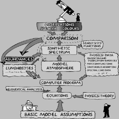
Figure 1: A cartoon that indicates the raison d’être for quantitative spectroscopy and the methodology

Figure 1 shows the methodology of quantitative spectroscopy in cartoon form. The basic goal is to produce detailed NLTE synthetic spectra, compare them to observations and then use those results to compare to theoretical predictions about the endpoint of stellar evolution models and explosions. We describe calculations performed using the multi-purpose stellar atmospheres program PHOENIX version 14 (Hauschildt and Baron, 1999; Baron and Hauschildt, 1998; Hauschildt et al., 1997a, b, 1996). PHOENIX solves the radiative transfer equation along characteristic rays in spherical symmetry including all special relativistic effects. The non-LTE (NLTE) rate equations for many ionization states are solved including the effects of ionization due to non-thermal electrons from the $\gamma$-rays produced by the radiative decay of ⁵⁶Ni, which is produced in the supernova explosion. For most of the calculations presented in this paper the atoms and ions calculated in NLTE are: H I, He I–II, C I-III, N I-III, O I-III, Ne I, Na I-II, Mg I-III, Si I–III, S I–III, Ca II, Ti II, Fe I–III, Ni I-III, and Co II. These are all the elements whose features make important contributions to the observed spectral features in SNe II.

Each model atom includes primary NLTE transitions, which are used to calculate the level populations and opacity, and weaker secondary LTE transitions which are are included in the opacity and implicitly affect the rate equations via their effect on the solution to the transport equation (Hauschildt and Baron, 1999). In addition to the NLTE transitions, all other LTE line opacities for atomic species not treated in NLTE are treated with the equivalent two-level atom source function, using a thermalization parameter, $\alpha=0.05$. The atmospheres are iterated to energy balance in the co-moving frame; while we neglect the explicit effects of time dependence in the radiation transport equation, we do implicitly include these effects, via explicitly including the rate of gamma-ray deposition in the generalized equation of radiative equilibrium and in the rate equations for the NLTE populations.

The models are parameterized by the time since explosion and the velocity where the continuum optical depth in extinction at 5000 Å ($\tau_{\mathrm{std}}$) is unity, which along with the density profile determines the radii. This follows since the explosion becomes homologous ($v\propto r$) quickly after the shock wave traverses the entire star. The density profile is taken to be a power-law in radius:

$$\rho\propto r^{-n}$$

where $n$ typically is in the range $6-12$. Since we are only modeling the outer atmosphere of the supernova, this simple parameterization agrees well with detailed simulations of the light curve (Blinnikov et al., 2000) for the relatively small regions of the ejecta that our models probe.

Further fitting parameters are the model temperature $T_{\mathrm{model}}$, which is a convenient way of parameterizing the total luminosity in the observer’s frame. We treat the $\gamma$-ray deposition in a simple parameterized way, which allows us to include the effects of nickel mixing which is seen in nearly all SNe II. Here we present preliminary results of modeling the nearby, well-observed, SN IIP 2005cs. More detailed results are presented in Ref. (Baron et al., 2006).

3 Reddening

Determining the extinction to SNe II is difficult, since they are such a heterogeneous class, it is difficult to find an intrinsic feature in the spectrum or light curve that can be used to find the parent galaxy extinction. Baron et al. (2003, 2000) found that the Ca II H+K lines can be used as a temperature indicator in modeling very early observed spectra. For SN 2005cs the reddening has been estimated in a variety of ways. Maund et al. (2005) used the relationship between the equivalent width of the Na I D interstellar absorption line to obtain a color excess of $E(B-V)=0.16$, as well as the color magnitude diagram of red supergiants within 2 arcsec of SN 2005cs to obtain $E(B-V)=0.12$, and their final adopted $E(B-V)=0.14$. Li et al. (2006) noted the large scatter in the relationships for equivalent width of the Na I D line, obtaining a range of $E(B-V)=0.05-0.20$. Assuming that the color evolution of SN 2005cs is similar to that of SN 1999em, they found $E(B-V)=0.12$. Also using the Na I D line Pastorello et al. (2006) found $E(B-V)=0.06$, but noting the uncertainty and comparing with the work of other authors they adopted $E(B-V)=0.11$. We began our work by adopting the reddening estimate of Pastorello et al. (2006), since our spectra were obtained from these authors. Figure 2 shows our best fit using solar abundances (Grevesse and Sauval, 1998) where the observed spectrum has been dereddened using the reddening law of Cardelli et al. (1989) and $R_{V}=3.1$. It is evident that the region around H$\beta$ is very poorly fit, there is a strong feature just to the blue of H$\beta$ and H$\beta$ itself is far too weak. We attempted to alter the model in a number of ways, changing the density profile, velocity at the photosphere, and gamma-ray deposition in order to strengthen H$\beta$, however we were unable to find any set of parameters that would provide a good fit to H$\beta$ (and the rest of the observed spectrum) with this choice of reddening. This model has $T_{\mathrm{model}}$ =18000 K, $v_{0}$ = 6000 $\mathrm{km}~{}\mathrm{s}^{-1}$, and $n=8$. Fig. 3 shows that if $T_{\mathrm{model}}$ is reduced to 12000 K and the color excess is reduced to the galactic foreground value of $E(B-V)=0.035$ (Schlegel et al., 1998) the fit is significantly improved. Our value of $E(B-V)=0.035$ is in agreement within the errors of the lower values found by Li et al. (2006) and Pastorello et al. (2006). Thus $E(B-V)=0.035-0.05$, but we will adopt the value of 0.035 for the rest of this work. This lower value of the extinction will somewhat lower the inferred mass of the progenitor found by Maund et al. (2005) and Li et al. (2006), but other uncertainties such as distance and progenitor metallicity also play important roles in the uncertainty of the progenitor mass. Clearly the bluest part of the continuum is better fit with the $T_{\mathrm{model}}$ =18000 K models than with the $T_{\mathrm{model}}$ =12000 K models. We did not attempt to fine tune our results to perfectly fit the bluest part of the continuum since the flux calibration at the spectral edges is difficult and it represents our uncertainty in $T_{\mathrm{model}}$  and $E(B-V)$. None of the above models have He I $\lambda 5876$ strong enough. It is well known that Rayleigh-Taylor instabilities lead to mixing between the hydrogen and helium shells, thus our helium abundance is almost certainly too low, but we will not explore helium mixing further.

Figure 2: Day 5: A synthetic spectrum using E(B-V) = 0.11, $T_{\mathrm{model}}$ = 18,000 K is compared to the observation.

Figure 3: Day 5: A synthetic spectrum using E(B-V) = 0.035, $T_{\mathrm{model}}$ = 12,000 K is compared to the observation.

4 Abundances

Typically, the approach to obtaining abundances in differentially expanding flows has been through line identifications. This method has been extremely successful using the SYNOW code (see Branch et al., 2005, 2006, and references therein) as well as the work of Mazzali and collaborators (for example Stehle et al., 2005). Nevertheless, line identifications do not provide direct information on abundances, which are what are input into stellar evolution calculations and output from hydrodynamical calculations of supernova explosions and nucleosynthesis. Line identifications are subject to error in that there may be another candidate line that is not considered in the analysis or there may be two equally valid possible identifications, the classic being He I $\lambda 5876$ and Na I D, which have very similar rest wavelengths and are both expected in supernovae (and have both been identified in supernovae).

Here we focus on nitrogen. Massive stars which are the progenitors of SNe II are expected to undergo CNO processing at the base of the hydrogen envelope followed by mixing due to dredge up and meridional circulation. This would lead to enhanced nitrogen and depleted carbon and oxygen. For our CNO processed models we take the abundances used by Dessart and Hillier (2005). However, significant mixing of the hydrogen and helium envelope is expected to occur during the explosion due to Rayleigh-Taylor instabilities and mass loss will occur during the pre-supernova evolution.

4.1 N II

N II lines were first identified in SN II in SN 1990E (Schmidt et al., 1993). Using SYNOW, Baron et al. (2000) found evidence for N II in SN 1999em, however more detailed modeling with PHOENIX indicated that the lines were in fact due to high velocity Balmer and He I lines. Prominent N II lines in the optical are N II $\lambda 4623$, $\lambda 5029$, and $\lambda 5679$. Dessart and Hillier (2005) found strong evidence for N II in SN 1999em. Using SYNOW Elmhamdi et al. (in preparation) found evidence for N II in SN 2005cs, as did Pastorello et al. (2006) using the code developed by Mazzali and collaborators. Figure 4 compares solar abundances to a model with enhanced CNO abundances (Dessart and Hillier, 2005; Prantzos et al., 1986). Figure 4 shows that the CNO enhanced abundances model does somewhat better fitting the emission peak of H$\beta$ (see § 4.2), however the feature to the blue of H$\beta$, clearly well-fit in the solar abundance model is completely absent in the model with enhanced CNO abundances. Figure 4 shows the region where the optical N II lines are prominent and in particular, the N II $\lambda 5679$ is not quite in the same place as the observed feature and the two bluer lines have almost no effect.

Figure 4: A synthetic spectrum using E(B-V) = 0.035, $T_{\mathrm{model}}$ = 12,000 K and enhanced CNO abundances is compared the solar model and to the observation. A blowup around the region where optical N II lines are prominent. The vertical dashed lines show the rest wavelength for the three lines, the vertical solid lines are blueshifted by 6000 $\mathrm{km}~{}\mathrm{s}^{-1}$.

4.2 Line IDs

In detailed line-blanketed models such as the ones presented here line identifications are difficult since nearly every feature in the model spectrum is a blend of many individual weak and strong lines. Nevertheless, it is useful to attempt to understand just what species are contributing to the variations in the spectra. In order to do this we produce “single element spectra” where we calculate the synthetic spectrum (holding the temperature and density structure fixed) but turning off all line opacity except for that of a given species. Figure 5 shows the single element spectrum for N II for our $T_{\mathrm{model}}$ = 12000 K models with CNO enhanced abundances. Clearly the N II lines are present in CNO enhanced models, but their effect on the total spectrum is unclear.

In an attempt to identify the better fit of the feature just to the blue of H$\beta$ we examined the single element spectrum of O II. Figure 6 clearly shows that O II lines play an important role in producing the observed feature just blueward of H$\beta$. Most likely it is the lines O II $\lambda 4651.5$ and $\lambda 4698$ which are producing the observed feature. On the other hand it is also clear that O II $\lambda 4915$ and $\lambda 4943$ are producing the deleterious feature just to the red of H$\beta$.

Thus, it is clear that the strong depletion of oxygen expected from CNO processing is not evident, we can not rule out that there is some enhanced nitrogen in the observed spectra, but the N II lines don’t seem to form in the right place. However since we are studying simple, parameterized, homogeneous models this could be an artifact of our parameterization. Nevertheless, the absorption trough of the feature that we would like to attribute to N II $\lambda 5679$ is too fast in our models, whereas one would expect the N II to be more enhanced on the outermost part of the envelope and thus to form at even higher velocity due to homologous expansion. Clumping could of course change this simple one-dimensional picture.

Figure 7 shows a preliminary synthetic spectrum compared to the observation 17 days after explosion and Fig. 8 shows the same for 34 days after explosion. Dessart & Hillier (this volume) find that time dependence in the rate equations is important for reproducing the Balmer lines. While our Balmer lines aren’t perfect they are quite reasonable and all relevant physical processes need to be included in the calculations.

Figure 5: CNO enhanced N II Single Element

Figure 6: Day 5: Solar O II Single Element

Figure 7: Day 17: A preliminary synthetic spectrum is compared to observation.

Figure 8: Day 34: A preliminary synthetic spectrum is compared to observation.

References

- Hauschildt and Baron (1999) P. H. Hauschildt, and E. Baron, J. Comp. Applied Math. 109, 41 (1999).
- Baron and Hauschildt (1998) E. Baron, and P. H. Hauschildt, ApJ 495, 370 (1998).
- Hauschildt et al. (1997a) P. H. Hauschildt, E. Baron, and F. Allard, ApJ 483, 390 (1997a).
- Hauschildt et al. (1997b) P. H. Hauschildt, G. Schwarz, E. Baron, S. Starrfield, S. Shore, and F. Allard, ApJ 490, 803 (1997b).
- Hauschildt et al. (1996) P. H. Hauschildt, E. Baron, S. Starrfield, and F. Allard, ApJ 462, 386 (1996).
- Blinnikov et al. (2000) S. Blinnikov, P. Lundqvist, O. Bartunov, K. Nomoto, and K. Iwamoto, ApJ 532, 1132 (2000).
- Baron et al. (2006) E. Baron, D. Branch, and P. H. Hauschildt, ApJ submitted (2006).
- Baron et al. (2003) E. Baron, P. E. Nugent, D. Branch, P. H. Hauschildt, M. Turatto, and E. Cappellaro, ApJ 586, 1199 (2003).
- Baron et al. (2000) E. Baron, et al., ApJ 545, 444 (2000).
- Maund et al. (2005) J. Maund, S. Smartt, and I. J. Danziger, MNRAS 364, L33–L37 (2005).
- Li et al. (2006) W. Li, S. D. Van Dyk, A. V. Filippenko, J.-C. Cuillandre, S. Jha, J. S. Bloom, A. G. Riess, and M. Livio, ApJ 641, 1060–1070 (2006), astro-ph/0507394.
- Pastorello et al. (2006) A. Pastorello, et al., MNRAS 370, 1752 (2006).
- Grevesse and Sauval (1998) N. Grevesse, and A. J. Sauval, Space Science Reviews 85, 161–174 (1998).
- Cardelli et al. (1989) J. A. Cardelli, G. C. Clayton, and J. S. Mathis, ApJ 345, 245 (1989).
- Schlegel et al. (1998) D. Schlegel, D. Finkbeiner, and M. Davis, ApJ 500, 525 (1998).
- Branch et al. (2005) D. Branch, E. Baron, N. Hall, M. Melakayil, and J. Parrent, PASP 117, 545–552 (2005), astro-ph/0503165.
- Branch et al. (2006) D. Branch, L. C. Dang, N. Hall, W. Ketchum, M. Melakayil, J. Parrent, M. A. Troxel, D. Casebeer, D. J. Jeffery, and E. Baron, PASP 118, 560–571 (2006), astro-ph/0601048.
- Stehle et al. (2005) M. Stehle, P. Mazzali, S. Benetti, and W. Hillebrandt, MNRAS 360, 1231 (2005).
- Dessart and Hillier (2005) L. Dessart, and D. J. Hillier, A&A 437, 667 (2005).
- Schmidt et al. (1993) B. Schmidt, et al., AJ 105, 2236 (1993).
- Prantzos et al. (1986) N. Prantzos, C. Doom, C. de Loore, and M. Arnould, ApJ 304, 695–712 (1986).