Predicting Photometric and Spectroscopic Signatures of Rings around Transiting Extrasolar Planets

Abstract

We present theoretical predictions for photometric and spectroscopic signatures of rings around transiting extrasolar planets. On the basis of a general formulation for the transiting signature in the stellar light curve and the velocity anomaly due to the Rossiter effect, we compute the expected signals analytically for a face-on ring system, and numerically for more general configurations. We study the detectability of a ring around a transiting planet located at $a=3$AU for a variety of obliquity and azimuthal angles, and find that it is possible to detect the ring signature both photometrically and spectroscopically unless the ring is almost edge-on (i.e., the obliquity angle of the ring $\theta$ is much less than unity). We also consider the detectability of planetary rings around a close-in planet, HD 209458b ($\theta\approx 90^{\circ}-i_{\rm orbit}\approx 3^{\circ}.32$), and Saturn ($\theta\approx 26^{\circ}.7$) as illustrative examples. While the former is difficult to detect with the current precision (photometric precision of $10^{-4}$ and radial velocity precision of 1 m s^-1), a marginal detection of the latter is possible photometrically. If the future precision of the radial velocity measurement reaches even below 0.1 m s^-1, they will be even detectable from the ground-based spectroscopic observations.

1 Introduction

In 1903, Hantaro Nagaoka, a professor in physics, Imperial University of Tokyo, proposed an atomic model which consists of a large number of particles of equal mass arranged in a circle at equal angular intervals around a central particle of large mass (Nagaoka, 1903, 1904). He referred to this model as a Saturnian model, and published the hypothesis prior to the famous Rutherford model (Rutherford, 1911), often referred to as a planetary model of the atom. This remarkable example in history illustrates how our Solar system, and even a Saturnian ring, inspired the best physicists in the world to contemplate the quantum world.

Thus it is interesting to contemplate how the properties of more than 300 extrasolar planets discovered so far beyond our Solar system will inspire future scientists. Among them, 52 systems are known to exhibit transiting signatures. Detailed photometric and spectroscopic observations of such transiting planets provide unique opportunities to look into the nature of extrasolar planets, which is otherwise unaccessible including the planetary radius, average density, and atmospheric composition. Ongoing/upcoming missions such as COROT and Kepler will significantly increase the number of transiting planets, and even a wider range of research will be made possible in the next several years. One specific example is the exploration of the spin-orbit misalignment of extrasolar planet using the Rossiter effect (Rossiter, 1924; McLaughlin, 1924; Petrie, 1938; Kopal, 1942, 1945; Hosokawa, 1953); when a planet transits its host star, the light coming from the star is partially blocked. Photometrically this produces a characteristic dimming of the stellar light curve, and spectroscopically, an asymmetric distortion of the absorption line profiles of the stellar spectrum due to the occultation of some of the velocity components of the stellar absorption lines. Thus the latter yields an apparent anomaly in the radial velocity curve of the host star (Queloz et al., 2000).

In a previous paper (Ohta, Taruya, & Suto, 2005, hereafter Paper I), we derived analytic templates for the velocity anomaly using a perturbative expansion. Motivated by that work, Winn et al. (2005) combined the best observational datasets currently available for the HD 209458 system, and detected for the first time a small misalignment ($\lambda=-4^{\circ}.4\pm 1^{\circ}.4$) between the spin axis of the central star and the orbital axis of the planet. Subsequently Wolf et al. (2006) applied the analytic formulae of Paper I, and obtained the limit, $\lambda=+11^{\circ}\pm 14^{\circ}$, for the anomalously dense planet, HD 149026 (Sato et al., 2005). Also, the spin-orbit alignment of the HD 189733 system were measured by Winn et al. (2006) and a very small misalignment of $\lambda=-1^{\circ}.4\pm 1^{\circ}.1$ was found (Winn et al., 2007a, b; Narita et al., 2007, see also). Recently measurements of spin-orbit alignment have been successful for a number of transiting planets. It is just a matter of time to obtain the statistical distribution of the misalignment angle $\lambda$, which provides a unique probe of the origin and evolution of the angular momentum of the planetary systems.

In the present paper, we consider an even more ambitious possibility to detect rings around transiting planets. It is interesting to note that the rings around Uranus and Neptune were indeed discovered during their occultation of background stars (Elliot, Dunham & Mink, 1977; Hubbard et al., 1977, 1986; Esposito, 2006). While it is not clear whether or not extrasolar planets have rings and/or satellites as those in our solar system, their detection, if successful, would definitely mark an important milestone in astronomy and planetary sciences; transiting planets are the unique targets for that purpose. From the methodology developed in this paper, one can further determine the orientation of the spin of the orbiting planet under a reasonable assumption that the orientation of the ring is aligned to the planetary spin axis; this is approximately the case for planetary rings in our Solar system.

Indeed we are not the first to explore the detectability in detail. Brown et al. (2001), for instance, put photometric constraints on possible satellites and rings around the first transiting planet, HD 209458b. They assume that an optically thick two-dimensional ring extending from the surface of the planet up to the outer radius $R_{\rm out}$. Hot Jupiters like HD 209458b are supposed to be roughly tidally locked to the host star. Thus they also assume that the ring plane coincides with the planetary orbital plane, and found that $R_{\rm out}$ should be less than 1.8 times the planetary radius. Given the approximate edge-on nature of the assumed ring, the upper limit is fairly strong and interesting. More recently Barnes & Fortney (2004, hereafter BF04) presented a light curve of ringed planets over a wide range of the parameter space, and discussed the photometric detectability of the additional ring signature.

Our present paper differs from the previous work in that we examine the spectroscopic detectability of planetary rings using the Rossiter effect in addition to the photometric one. Given the current observational sensitivities, the photometric signatures are easier to detect than the spectroscopic ones in most cases. Nevertheless, the complementary nature of the spectroscopic detection/confirmation of rings is important because the signature of rings is very subtle and may be mimicked/disguised by unknown noise and systematics. Moreover the spectroscopic signature may be more pronounced for transiting planets in rapidly rotating stars because the velocity anomaly due to the Rossiter effect is simply proportional to the stellar spin velocity.

We also present improved and more accurate analytic formulae of the photometric light curve and the spectroscopic velocity anomaly for a transiting planet without a ring than those in Paper I. While those for a planet with a ring need to be computed numerically in general, such analytic formulae are very useful in performing the parameter fit for a ringless planet model, and also in checking the accuracy of the numerical results for a planet with a ring.

The plan of the paper is as follows; we describe our basic assumptions for the planet and ring system in §2. Section 3 summarizes the general formulation to compute the photometric and spectroscopic signals for the planet and ring system. Analytical results for the face-on ring are presented in §4, which are in fact the improved version of the results of Paper I. Numerical results for an arbitrarily oriented ring are shown in §5, and we discuss its detectability in detail. Finally §6 is devoted to conclusions and implications of the paper.

2 Model assumptions

Let us begin with describing several definitions and assumptions concerning the geometrical configuration of the planetary system and the properties of the host star, the orbiting planet and a surrounding ring. Table 1 lists the notations and the parameters of our model, which are used in the analysis below.

Figure 1: Planetary transit accompanied by a ring. The internal parameters of the star and the planet are shown: stellar radius $R_{s}$; projected angular velocity $\Omega_{s}\,\sin I_{s}$; impact parameter of planetary orbit, $b$; angle between the $x$-axis and the orbital plane, $\lambda$, which represents the spin-orbit alignment projected onto the $x-z$ plane.

2.1 Star–planet system

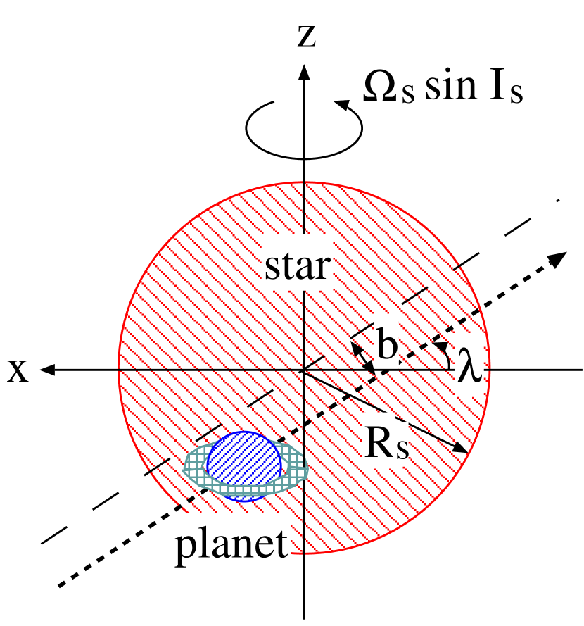
We assume that the star (radius $R_{s}$) and the planet (radius $R_{p}$) follow the exact two-body Kepler orbit, ignoring perturbations from possible outer planets. We adopt a coordinate system centered at the star so that its $y$-axis is directed toward the observer, and the $z$-axis is chosen so that the stellar rotation axis lies on the $y$-$z$ plane. We assume rigid-body stellar rotation with $\Omega_{s}$ being its spin angular velocity. In this coordinate system, the components of the stellar spin angular velocity reduces to

$${\bf\Omega}_{s}=(0,\Omega_{s}\cos I_{s},\Omega_{s}\sin I_{s}),$$ (1)

where $I_{s}$ is the inclination angle between the stellar spin axis and observer’s direction.

Since we are mainly interested in the transit phase whose duration is much shorter than the entire orbital period, the actual eccentric orbit is close to a circular one in the vicinity of the planetary transit. Thus we adopt the circular orbit in the present analysis while most of our formulae below are applicable to a non-circular orbit by properly mapping the projected position of the planet into the observed time. Under the circular orbit approximation, the planetary orbit is simply characterized by the impact parameter $b$ and the projected angle $\lambda$ between the stellar spin and the planetary orbital axes, in addition to the semi-major axis $a$ (Fig. 1). The impact parameter $b$ is equal to $b=a\cos i_{\rm orbit}/R_{s}$, where $i_{\rm orbit}$ is the inclination of the orbit.

We adopt the linear limb darkening alone for the surface intensity of a stellar disk in Paper I. In this paper, we take account of the effect up to quadratic order:

$$I_{\rm star}(\mu)=I_{0}\left[1-u_{1}(1-\mu)-u_{2}(1-\mu)^{2}\right].$$ (2)

The two constants, $u_{1}$ and $u_{2}$, characterize the amplitude of the limb darkening, and $\mu$ is the directional cosine between the line of sight and the normal vector to the local stellar surface:

$$\mu=\sqrt{1-\frac{x^{2}+z^{2}}{R_{s}^{2}}}.$$ (3)

2.2 Planet and ring

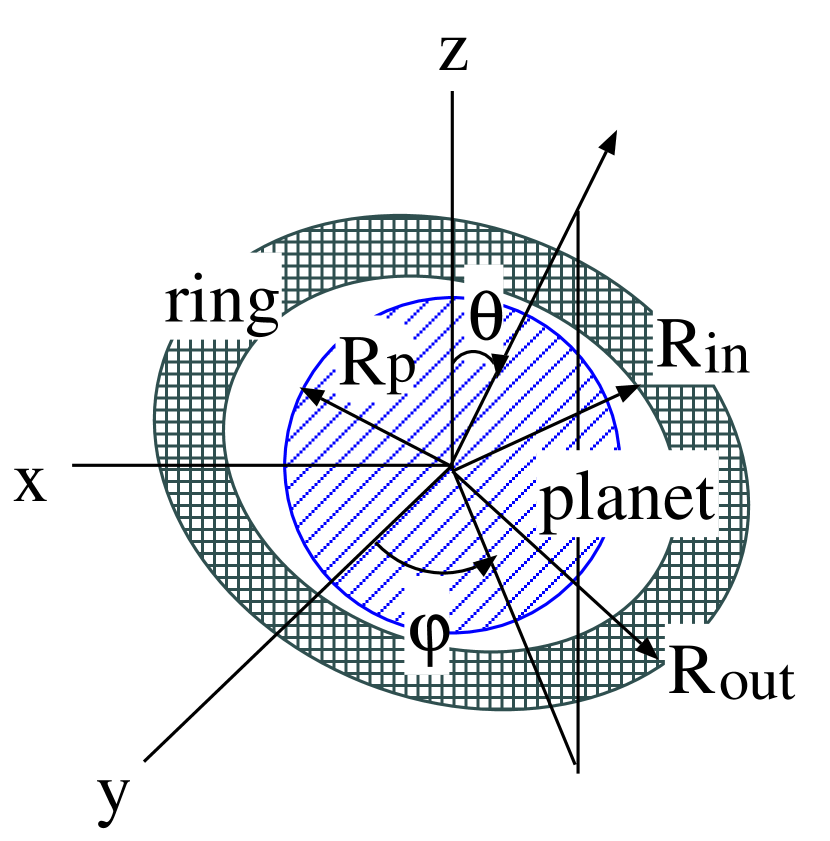
We consider a simple model of ring around a planet as shown in Figure 2. The ring is two-dimensional (geometrically thin) and circular. Its inner and outer radii are denoted by $R_{\rm in}$ and $R_{\rm out}$ which satisfy $R_{p}<R_{\rm in}<R_{\rm out}$. We assume that the ring moves along the planetary orbit with constant obliquity angles $(\theta,\phi)$. The light transmitted through the ring diminishes due to the absorption and/or the extinction by particles in the ring. We introduce the normal optical depth of ring, $\tau$, so that the transmitted flux through the ring is proportional to $\exp(-\tau/\beta)$, where $\beta$ is the cosine of the angle between the normal vector to the ring surface and $y$-axis, and given by $\beta=\sin\theta\cos\phi$. We adopt $\tau=1$ for simplicity (see Table 1); the optical depth of the B ring of Saturn is in the range of $\tau=0.4\sim 2.5$ (Murray & Dermott, 1999).

Figure 2: Schematic configuration of the planet accompanied by a ring. The parameters of the planet and the ring include planetary radius $R_{p}$, radius of inner edge of ring $R_{\rm in}$, radius of outer edge of ring $R_{\rm out}$, obliquity angle $\theta$ (the angle between the normal vector to the ring surface and $z$-axis), rotation angle $\phi$ (the angle between the $y$-axis and the projected normal vector of ring surface onto the $y-z$ plane).

Barnes & Fortney (2004) examined the influence of diffraction on the photometric light curves, and found that it may leave a detectable signature depending on the size of ring particles. We ignore the diffraction of the ring particles here for two reasons; first, our primary purpose is to develop a methodology which directly tests the presence of rings, and second, the diffraction effect itself does not exceed the primary effect of the star-light dimming. In any case the effect of diffraction can be easily incorporated into our numerical scheme if the ring properties are specified.

3 Photometric and spectroscopic transit signatures for a planet with a ring

3.1 Photometric signals

The photometric light curve for transiting extrasolar planet with a ring has been computed by Barnes & Fortney (2004) in detail. For definiteness and later convenience, we summarize their basic equations in terms of our own notations here.

The dimming of the star light during the transit phase is quantified by evaluating the fraction of star light blocked by the planet and/or intercepted the ring. We define the relative flux ratio $F$:

$$F=\frac{\displaystyle\int\!\!\!\int I(x,z)dxdz}{\displaystyle\int\!\!\!\int I_{\rm s}(x,z)dxdz}.$$ (4)

Here, the functions $I(x,z)$ and $I_{\rm s}(x,z)$ represent an intensity at a given position $(x,z)$ of the stellar surface. The stellar intensity model (2) and the ring model described in §2.2 yield the explicit form of the function $I(x,z)$:

$$I(x,z)=\left\{\begin{array}[]{lcl}0&:&\mbox{region outside the star, i.e.,~{} }x^{2}+z^{2}>R_{s}^{2}\\ 0&:&\mbox{region inside the planet, i.e.,~{} }(x-X_{p})^{2}+(z-Z_{p})^{2}\leq R_{p}^{2}\\ e^{-\tau/\beta}I_{\rm star}(\mu)&:&\mbox{region transmitted through the ring, see}~{}~{}{\rm conditions\,\,(\ref{eq:ring_transmit_cond})}\\ I_{\rm star}(\mu)&:&\mbox{otherwise}\end{array}\right.,$$ (9)

where the direction cosine $\mu$ is given by equation (3). The region where the light coming from the star is transmitted through the ring satisfies the three conditions:

$$\left\{\begin{array}[]{l}R_{\rm in}^{2}<\left(\displaystyle\frac{x-X_{p}-(z-Z_{p})\sin\phi}{\cos\phi}\right)^{2}+\left(\displaystyle\frac{z-Z_{p}}{\sin\theta}\right)^{2}<R_{\rm out}^{2},\\ x^{2}+z^{2}<R_{s}^{2},\\ (x-X_{p})^{2}+(z-Z_{p})^{2}>R_{p}^{2}\end{array}\right.$$ (13)

The quantities, $X_{p}$ and $Z_{p}$, represent the position centered at the planet, which manifestly depend on time.

The stellar intensity outside the transit phase, $I_{\rm s}(x,z)$, is simply written as

$$I_{\rm s}(x,z)=\left\{\begin{array}[]{lcl}0&:&\mbox{outside the star i.e., }x^{2}+z^{2}>R_{s}^{2}\\ I_{\rm star}(\mu)&:&\mbox{inside the star i.e., }x^{2}+z^{2}<R_{s}^{2}\end{array}\right..$$ (16)

Substituting the stellar intensity model (2), the denominator of equation (4) can be integrated analytically:

$$\int\!\!\!\int I_{s}(x,z)dxdz=\pi I_{0}R_{s}^{2}\left(1-\frac{u_{1}}{3}-\frac{u_{2}}{6}\right).$$ (17)

Note that this is independent of time.

3.2 Spectroscopic signals

While planetary rings may be detectable with photometric data analysis alone, the spectroscopic data provide an independent and complementary check of the presence of rings. Since the two methods would suffer from very different noises and systematics, the agreement between them significantly increases the credibility of the positive detection.

The spectroscopic detection method relies on the Rossiter effect (Rossiter, 1924) which represents the “apparent” radial velocity modulation arising from the spectral line distortion due to an occultation of a part of the rotating star. During the passage of the transiting planet, the light from the stellar surface is asymmetrically blocked off. As a result, the line-profile-weighted mean position for a specific absorption or emission line taking account of the stellar rotation is apparently shifted. In Paper I, we derived analytical expressions for radial velocity curves for extrasolar transiting planets for the first time, but the effect of rings was ignored. The quantitative modelling of the photometric and spectroscopic signatures of rings will be considered in detail below.

Formally the radial velocity anomaly due to the Rossiter effect is expressed as

$$\Delta v_{s}=-\Omega_{s}\sin I_{s}\frac{\displaystyle\int\!\!\!\int x\,\,I(x,z)dxdz}{\displaystyle\int\!\!\!\int I(x,z)dxdz}.$$ (18)

The above expression, which relates the velocity anomaly to the first moment of the line profile, is applicable also to transiting planets with a ring if equation (9) is substituted into $I(x,z)$. In general, the above integral cannot be performed analytically but needs to be done numerically (except for a face-on ring as described in §4). We note here that Winn et al. (2005) pointed out the presence of $\sim 10$ percent systematic difference between the perturbative results of Paper I and their numerical fits to the outputs of the data analysis pipeline. This is supposed to come from the fact that the approximation of the first moment of the line profile as $\Delta v_{s}$ is not sufficiently accurate. The systematic difference should be sensitive to the specific data analysis routine, and hard to evaluate generally. Moreover it is unlikely to affect our conclusions which depend on the difference of $\Delta v_{s}$ of planets with and without rings. This is why we use equation (18) to evaluate the Rossiter effect in what follows.

In practice, we proceed as follows; we first calculate the integral over an entire surface of the stellar disk, which can be done analytically. Then we numerically evaluate the integrals over the regions overlapped with the planet and the ring, and subtract these from the analytic result without a planet nor a ring. In order to cope with the complicated geometry of the integration, we set square grids ($256\times 256$ cells) enclosing both the planet and the ring with a length of $2R_{\rm out}$ on a side. Judging from the location of the center of each cell relative to the stellar surface, we assign the intensity $I(x,z)$ in equation (9), and compute the contribution from the cell. We test the convergence and the accuracy of our numerical integrations by comparing with the results with finer grids ($512\times 512$ cells). We find that the fractional difference of the photometric signal is less than $3\times 10^{-5}$, and that the spectroscopic signals agree within $0.08{\rm ms^{-1}}$, both of which are negligibly small for our current purpose.

4 Analytic formulae for a planet with a face-on ring

Equations (4) and (18) can be integrated (almost) analytically for a planet with a face-on ring, i.e., $(\theta,\,\phi)=(90^{\circ},\,0^{\circ})$. These analytic formulae help our understanding of the basic observational signatures of a ring from the photometric and the spectroscopic data. They are also useful in making sure of the accuracy of the numerical results for more general cases.

We find that equation (4) reduces to

$$F=\frac{\displaystyle\pi(1-u_{1}/3-u_{2}/6)-A(\rho,\gamma_{\rm ps})-(1-e^{-\tau})\left\{A(\rho,\gamma_{\rm os})-A(\rho,\gamma_{\rm is})\right\}}{\pi(1-u_{1}/3-u_{2}/6)}$$ (19)

for the relative flux ratio, and equation (18) to

$$\Delta v_{s}=X_{p}\,\,\Omega_{s}\,\sin I_{s}\,\,\frac{\displaystyle B(\rho,\gamma_{\rm ps})+(1-e^{-\tau})\left\{B(\rho,\gamma_{\rm os})-B(\rho,\gamma_{\rm is})\right\}}{\displaystyle\pi(1-u_{1}/3-u_{2}/6)-A(\rho,\gamma_{\rm ps})-(1-e^{-\tau})\left\{A(\rho,\gamma_{\rm os})-A(\rho,\gamma_{\rm is})\right\}}.$$ (20)

for the radial velocity shift, where $\gamma_{\rm ps}=R_{p}/R_{s}$, $\gamma_{\rm is}=R_{\rm in}/R_{s}$, $\gamma_{\rm os}=R_{\rm out}/R_{s}$, and $\rho\equiv\sqrt{X_{p}^{2}+Z_{p}^{2}}/R_{s}$. The quantities, $A$ and $B$, are given in terms of the normalized planet position $\rho$ as follows:

$$A(\rho,\,\gamma)=\left\{\begin{array}[]{lcl}\pi\gamma^{2}\left[1-u_{1}-u_{2}\left(2-\rho^{2}-\gamma^{2}/2\right)+(u_{1}+2u_{2})W_{1}\right]&:&\rho<1-\gamma\\ \\ \left(1-u_{1}-3u_{2}/2\right)\left[\gamma^{2}\cos^{-1}\left(\zeta/\gamma\right)+\sin^{-1}z_{0}-\rho z_{0}\right]&&\\ \quad+(u_{2}/2)\,\rho\left[(\rho+2\zeta)\gamma^{2}\cos^{-1}\left(\zeta/\gamma\right)-z_{0}\left(\rho\zeta+2\gamma^{2}\right)\right]&:&1-\gamma\leq\rho\leq 1+\gamma\\ \quad\quad+(u_{1}+2u_{2})W_{3}&&\\ \\ 0&:&1+\gamma<\rho\end{array}\right.$$ (28)

and

$$B(\rho,\,\gamma)=\left\{\begin{array}[]{lcl}\pi\gamma^{2}\left[1-u_{1}-u_{2}\left(2-\rho^{2}-\gamma^{2}\right)+(u_{1}+2u_{2})W_{2}\right]&:&\rho<1-\gamma\\ \\ \left[1-u_{1}-u_{2}\left(2-\rho^{2}-\gamma^{2}\right)\right]\left[\gamma^{2}\cos^{-1}\left(\zeta/\gamma\right)-z_{0}\zeta\right]&&\\ \quad-(4u_{2}/3)\rho z_{0}^{3}+(u_{1}+2u_{2})W_{4}/\rho&:&1-\gamma\leq\rho\leq 1+\gamma\\ \\ 0&:&1+\gamma<\rho\end{array}\right.$$ (35)

The variables $z_{0}$ and $\zeta$ are also written in terms of $\gamma$ and $\eta_{p}=\rho-1$ as

$$z_{0}(\gamma)=\frac{\sqrt{(\gamma^{2}-\eta_{p}^{2})\Bigl{[}(\eta_{p}+2)^{2}-\gamma^{2}\Bigr{]}}}{2(1+\eta_{p})},\quad\quad\zeta(\gamma)=\frac{\eta_{p}^{2}+2\eta_{p}+\gamma^{2}}{2(1+\eta_{p})}.$$ (36)

The functions $W_{i}$ ($i=1\sim 4$) in the above expressions are in fact analytically intractable, but we find accurate analytical fitting formulae which are explicitly given in Appendix A.

If we set $\tau=0$, the above analytic expressions reduce to a case of a planet without a ring. However they are superior to, and thus should replace, our previous results (Ohta, Taruya, & Suto, 2005) in two ways; first, we now consider a quadratic limb darkening (eq.[2]), instead of a linear limb darkening ($u_{2}=0$), and second, the approximate expressions for $W_{i}$ given in the appendix are more accurate by a factor of a few than the previous one; for typical parameters $\gamma_{\rm ps}\leq\gamma_{\rm is}\leq\gamma_{\rm os}\sim 0.2$, the accuracy is typically within a few percent level. We use the above formulae extensively when we discuss the effect of rings in the following analysis.

5 Predicted photometric and spectroscopic signals

Even in the simple model that we assume here, the photometric light curve and the spectroscopic velocity curve are characterized by 12 and 14 parameters, respectively. The former includes the radii of the star and the planet ($R_{s}$ and $R_{p}$), the inner and the outer edges of the ring ($R_{\rm in}$ and $R_{\rm out}$), the limb-darkening parameters ($u_{1}$ and $u_{2}$), the orbital parameters of the system (semi-major axis $a$, inclination of the orbital plane $i_{\rm orbit}$, and the orbital rotation period $P_{\rm orbit}$), the obliquity angles of the ring ($\theta$ and $\phi$), and finally the normal optical depth of the ring, $\tau$. The additional two parameters for the latter are the projected stellar surface velocity $V\sin I_{s}$ and the projected misalignment angle $\lambda$ between the stellar spin and the orbital plane axes.

In order to avoid the tidal disruption, the outer radius of the ring should not exceed the Hill radius:

$$R_{\rm out}<r_{\rm H}=\left(\frac{M_{p}}{3M_{s}}\right)^{1/3}a\approx 15.4R_{J}\left(\frac{M_{p}}{M_{J}}\right)^{1/3}\left(\frac{M_{\odot}}{M_{s}}\right)^{1/3}\left(\frac{a}{0.05{\rm AU}}\right).$$ (37)

Gaudi, Chang & Han (2003) discussed further theoretical constraints on planetary rings. Planetary rings consisting of ice sublimation if the planetary semi-major axis satisfies

$$a>\left(\frac{L_{*}}{16\pi\sigma T_{\rm sub}^{4}}\right)^{1/2}=2.7{\rm AU}\left(\frac{L_{*}}{L_{\odot}}\right)^{1/2},$$ (38)

where $T_{\rm sub}=170{\rm K}$ is the sublimation temperature of water ice, and $L_{*}$ is the luminosity of the host star. For rocky rings, the Poynting Robertson drag force, viscous friction due to the planetary exosphere, torques due to (shepherd) satellites, and internal scattering become important. For close-in planets, the Poynting Robertson drag time-scale $t_{\rm PR}$ is generally shorter than the viscous friction decay time-scale unless the density of the exosphere is large, $\rho_{\rm es}\lower 2.15277pt\hbox{$\;\buildrel>\over{\sim}\;$}10^{-16}{\rm gcm^{-3}}$ (Goldreich & Tremaine, 1982). The former is given as

$$t_{\rm PR}\sim 10^{5}{\rm yr}\frac{\rho}{1{\rm gcm^{-3}}}\frac{r}{1{\rm cm}}\left(\frac{a}{0.1{\rm AU}}\right)^{2},$$ (39)

where $\rho$ and $r$ denote the density and the radius of ring particles. Thus rings around close-in planets would not live longer than $t_{\rm PR}$ unless any stabilization mechanism like shepherd satellites operates. Thus it is not clear if close-in planets are accompanied by rings.

Based on these estimates, we adopt a fiducial set of parameters listed in Table 1, which is motivated by the existing close-in planetary system HD 209458, but with different semi-major axis, $a=3$AU. As illustrative examples, we also consider the close-in planet and the Saturn system as a member of solar-system planet. We first present a special case of the face-on ring (that can be analytically computed) so as to elucidate the basic features (§5.1), and to quantify the parameter dependence of the photometric and spectroscopic signals in §5.2. Next in §5.3, we discuss how to identify the signature of rings by looking for the departure from the fit to a planet model without ring. Based on these discussions, the detectability of a ring system is addressed in §5.4, in addition to future prospects for constraining the ring parameters.

5.1 Signature of the face-on ring

Figure 3: Schematic illustration for photometric and spectroscopic signatures of transiting planet with and without a ring (see Table 1 for the fiducial values of the model parameters). The top panel shows the velocity anomaly curve for the Rossiter effect. The ring is assumed to be face-on, i.e., $\theta=90^{\circ}$, $\phi=0^{\circ}$. The curve is analytically calculated according to the expression (20). The bottom panel shows the light curve during transit. The ring is also face-on. The curve is analytically calculated according to the expression (19).

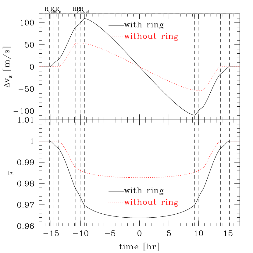
Figure 3 shows the velocity anomaly by the Rossiter effect (upper) and the light curve of photometry (lower) for a planet with a face-on ring, i.e., $\theta=\varphi=0$. The central transit time is chosen as $t=0$. These curves are plotted using the analytical expressions (19) and (20).

Compared to the curves of a planet without a ring (dashed lines), the planetary ring produces larger radial velocity shifts and flux dimming (solid lines). Also the transit duration increases. As we will show below, however, most of those features due to the ring resemble that of a ringless planet with a larger radius. The vertical dotted lines in Figure 3 indicate the epochs when the boundary edges of the planet and the ring contact the edge of the stellar disk (i.e., the ingress and egress phases). These somewhat discontinuous features in the derivatives of the curves, if detectable directly at all, would be an unambiguous confirmation of the presence of the ring. In reality, however, it may be difficult to locate the features from the sampled data with a finite exposure time.

A more realistic methodology is to first search for the best-fit parameters assuming no ring at all, and then to look for any systematic ring signatures in the residuals between the observed data and the fits (Barnes & Fortney, 2004). Even so, the detection of rings requires better resolutions in sampling time, as well as in photometric and spectroscopic accuracy, than those of current data.

5.2 Dependence on the ring parameters

Figure 4: Same as Figure 3, but for a ring with different set of parameters. The top panel shows the velocity anomaly from Rossiter effect, while bottom panel plots the light curve during transit. In each panel, solid lines represent the results for the fiducial model (Table 1). Other lines show the results when one of the fiducial parameters is varied; $\theta=70^{\circ}$ (dotted), $\phi=45^{\circ}$ (short-dashed), $R_{\rm in}=R_{p}$ (long-dashed), and $R_{\rm out}=2.5R_{p}$ (dot-dashed).

Figure 5: Variation of the photometric (upper) and spectroscopic (lower) signals with respect to the ring parameters, $R_{\rm in}$, $R_{\rm out}$, and $\theta$. The curves for the latter case are multiplied by a factor of 10 for clarity.

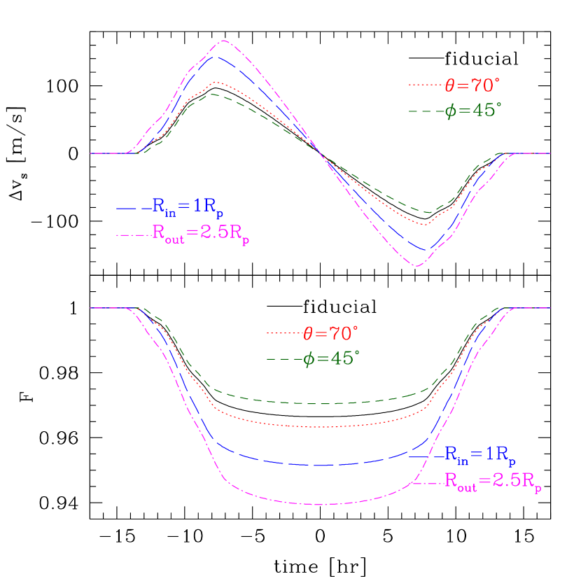
In general, the photometric and the spectroscopic signals due to rings need to be evaluated numerically. Here we discuss their sensitivity on the four ring parameters ($\theta,\varphi,R_{\rm in}$ and $R_{\rm out}$). Figure 4 shows some examples with slightly different parameters from our fiducial values; $\theta=45^{\circ}\to 70^{\circ}$ (dotted), $\phi=0^{\circ}\to 45^{\circ}$ (short-dashed), $R_{\rm in}=1.5R_{p}\to 1.0R_{p}$ (long-dashed) and $R_{\rm out}=2.0R_{p}\to 2.5R_{p}$ (dot-dashed).

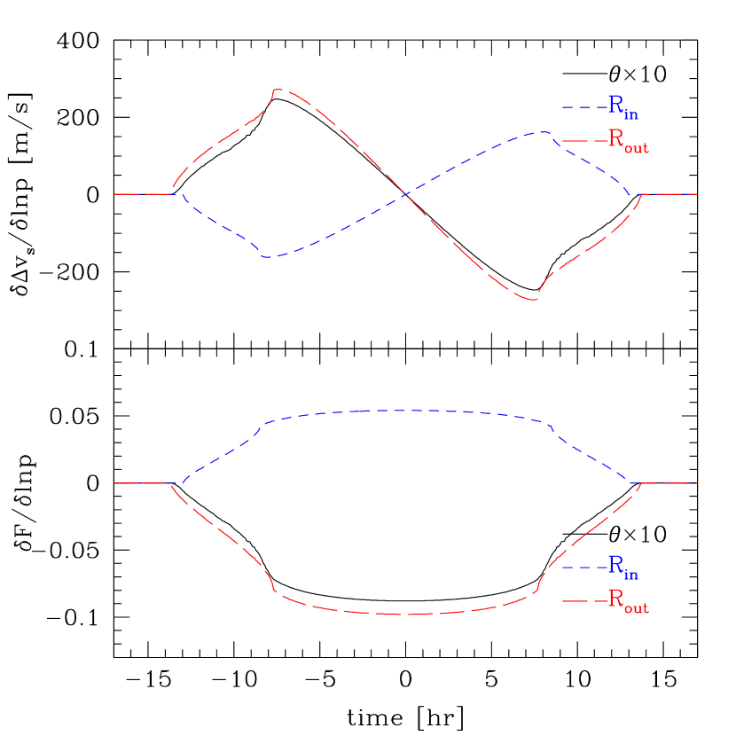
In order to clarify how the predicted $\Delta v_{s}$ and $F$ are sensitive to the underlying parameters of the system ($\theta$, $\phi$, $R_{\rm in}$ and $R_{\rm out}$), we compute their dependence as we did in Figure 9 of Paper I. Specifically, Figure 5 illustrates the variation of the radial velocity shifts $\Delta v_{s}$ with respect to $p=R_{\rm in}$, $R_{\rm out}$ and $\theta$:

$$\frac{\delta\Delta v_{s}}{\delta\ln p}\equiv\lim_{dp\rightarrow 0}\frac{\Delta v_{s}(p+dp;t)-\Delta v_{s}(p;t)}{dp/p}.$$ (40)

Similarly we define the variation of the photometric light curves $\delta F$:

$$\frac{\delta F}{\delta\ln p}\equiv\lim_{dp\rightarrow 0}\frac{F(p+dp;t)-F(p;t)}{dp/p},$$ (41)

which are also plotted in Figure 5. Since the dependence on $\theta$ is small, we multiply the values of $\delta\Delta v_{s}/\delta\ln\theta$ and $\delta F/\delta\ln\theta$ by a factor of 10 in the plot.

Figure 4 indicates that a different set of the ring parameters mainly changes the amplitude of signals during the full transiting phase, and that the bumpy structures around the ingress and the egress phases, which indeed are the important signatures of possible rings, are not affected much. This can be understood from the weak dependence on the angle parameters in Figure 5. If we changes the value of one of the ring parameters from $p$ to $p^{\prime}$, the photometric and spectroscopic signals become

$$F(p^{\prime};t) \approx F(p;t)+\left(\frac{p^{\prime}-p}{p}\right)\frac{\delta F}{\delta\ln p},$$ (42)

$$\Delta v_{s}(p^{\prime};t) \approx \Delta v_{s}(p;t)+\left(\frac{p^{\prime}-p}{p}\right)\frac{\delta\Delta v_{s}}{\delta\ln p}.$$ (43)

Those approximate perturbation formulae combined with Figure 5 explain the behavior of Figure 4 fairly well, in particular the weak dependence on $\theta$.

We note that the three ring parameters ($\theta,R_{\rm in}$ and $R_{\rm out}$) symmetrically change the photometric light curves around the central transit time and anti-symmetrically change the radial velocity shifts (Fig.5). Such behavior is quite similar to the variation with respect to the planetary and the stellar internal parameters (see Fig.9 of Paper I). Thus, the overall change of the amplitude is not a sensitive measure of the presence of a ring. Therefore the precise measurement of the bumps around the ingress and the egress phases, even if difficult, provides the key in the detection and the characterization of the planetary ring.

5.3 Signatures of rings

The results of the previous subsections now enable us to discuss in detail the signatures of a ring system in photometric and spectroscopic data. Given real data set, first thing that we should do is to fit the photometric light curve and/or the spectroscopic velocity anomaly of a transit planet using a model without ring. If the residuals between the data and the best-fit model are significantly larger than the observational errors, one suspects the presence of a ring.

More specifically, let us introduce the above residuals as

$$\mbox{Res}[v_{s}]\equiv\Delta v_{s}^{\rm obs}-\Delta v_{s}^{\rm best-fit}~{}(\mbox{without ring})$$ (44)

and

$$\mbox{Res}[F]\equiv F^{\rm obs}-F^{\rm best-fit}~{}(\mbox{without ring}).$$ (45)

Lovis et al. (2006) has already achieved $\sim 1$m s^-1 sensitivity in the radial velocity measurement. Also the HST photometric accuracy is shown to be better than $0.1$% (Brown et al., 2001), which is expected to be the case for upcoming space missions as well. Figure 6 illustrates examples for $\mbox{Res}[v_{s}]$ and $\mbox{Res}[F]$; the upper and lower-left panels show our fiducial ring model (Table 1) with three different orientations, ($\theta=45^{\circ},\phi=0^{\circ}$), ($\theta=90^{\circ},\phi=0^{\circ}$) and ($\theta=90^{\circ}-i_{\rm orbit}=3^{\circ}.32,\phi=0^{\circ}$). The last case corresponds to a close-in planet, HD 209458b, with ring. The semi-major axis and inclination angle of the orbital plane with respect to our line-of-sight are set to $a=0.0468$AU and $i_{\rm orbit}=86^{\circ}.68$, respectively. Since close-in planet is likely to be a tidally-locked system, we assume that the ring plane lies in the planetary orbital plane. Thus, $\theta$ is equal to $90^{\circ}-i_{\rm orbit}$. The lower-right panel is intended to illustrate the expected signals for the Saturn system (B-ring) just for comparison; $\theta=26^{\circ}.7,\phi=0^{\circ}$, $R_{\rm in}=1.53R_{\rm Saturn}$, $R_{\rm out}=1.95R_{\rm Saturn}$, $V\sin I_{s}=1,880{\rm m}\,{\rm s}^{-1}$. Note that in the lower panels, the residuals obtained from the numerical fit are also plotted as dashed lines, in addition to the results from the analytical fit (solid). The residuals, $\mbox{Res}[v_{s}]$ and $\mbox{Res}[F]$, clearly indicate the characteristic pattern expected for a ring. More importantly, the above signatures are indeed at a few $\sigma$ level of the currently best observational sensitivities, both photometrically and spectroscopically. Even though it is not clear if those values that we adopted for the ring parameters are realistic, the result is certainly encouraging.

Figure 6: Spectroscopic and photometric signatures of a ring. Each panel displays the velocity anomaly due to the Rossiter effect $\Delta v_{s}$, the spectroscopic residual $\mbox{Res}[v_{s}]$, photometric light curve $F$, and the photometric residual $\mbox{Res}[F]$ from top to bottom. Solid and dashed curves in $\Delta v_{s}$ and $F$ present our predictions and the best-fit without ring model. Note that in lower panels, the residuals obtained from the numerical fit are also plotted as dashed lines, in addition to the one obtained from the analytical fit (solid) ; $\theta=45^{\circ},\phi=0^{\circ}$ (upper-left), $\theta=90^{\circ},\phi=0^{\circ}$ (upper-right), tidally-locked close-in planet adopting the orbital parameters of HD 209458 system, i.e., $a=0.0468$AU, $\theta=3^{\circ}.32,\phi=0^{\circ}$ (lower-left), and Saturn system (B-ring) with $\theta=26^{\circ}.7,\phi=0^{\circ}$, $R_{\rm in}=1.53R_{\rm Saturn}$, $R_{\rm out}=1.95R_{\rm Saturn}$, $V\sin I_{s}=1,880\,{\rm m}\,{\rm s}^{-1}$ (lower-right).

Figure 7: Same as the upper-left panel of Figure 6, but with a different parameter set; $\theta=70^{\circ}$ (upper-left), $\phi=45^{\circ}$ and $i_{\rm orbit}=89^{\circ}.95$ (upper-right), and $R_{\rm in}=1R_{p}$ (lower-left) and $R_{\rm out}=2.5R_{p}$ (lower-right).

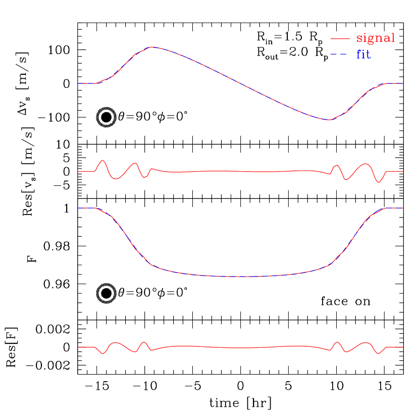
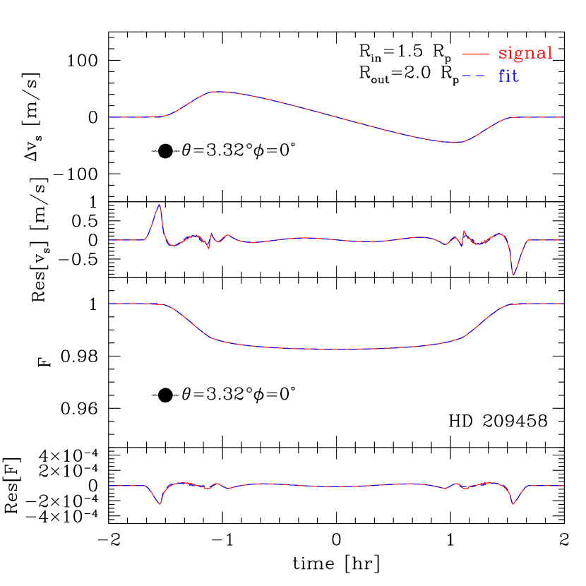
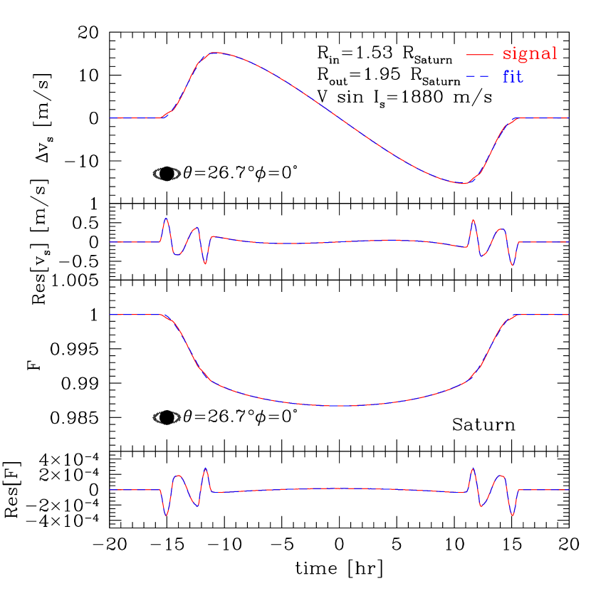
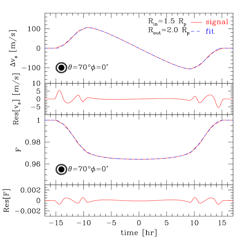
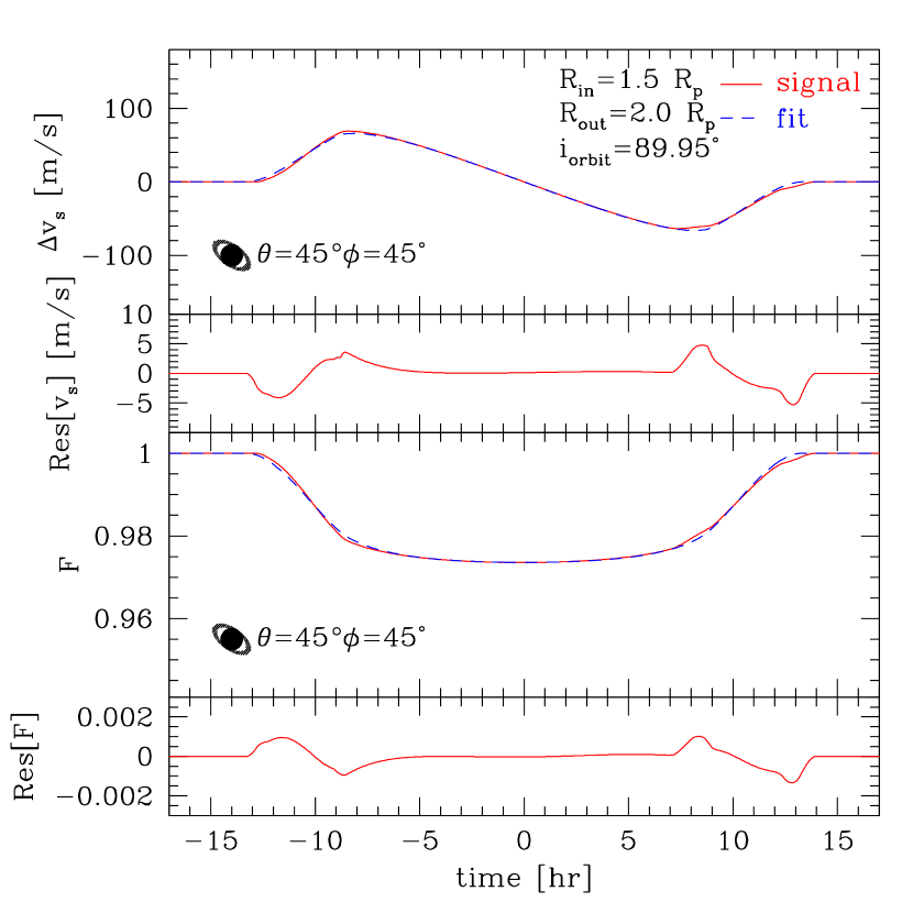
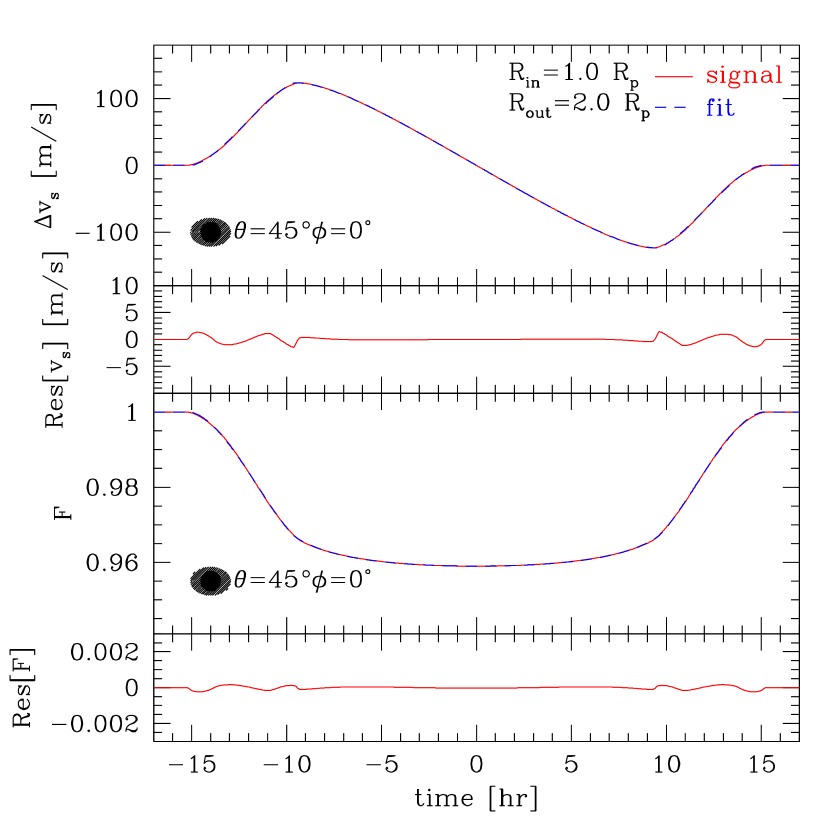
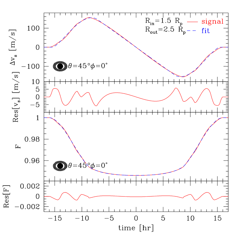
Figure 7 displays the results when one parameter of the ring system is changed from the fiducial values, $\theta=45^{\circ},\phi=0^{\circ}$, $R_{\rm in}=1.5R_{\rm p}$, and $R_{\rm out}=2.0R_{\rm p}$ (the upper-left panel of Fig.6); $\theta=70^{\circ}$ (upper-left), $\phi=45^{\circ}$ and $i_{\rm orbit}=89^{\circ}.95$(upper-right), and $R_{\rm in}=1.0R_{\rm p}$ (lower-left) and $R_{\rm out}=2.5R_{\rm p}$ (lower-right). The behavior is fairly easy to understand in an intuitive manner. As long as the clear gap between the planetary surface and the inner edge of the ring exists, a ring produces a larger residual as $\theta$ approaches $90^{\circ}$ (face-on); an edge-on system is hard to identify. A non-zero value of $\phi$ generates an asymmetry in the residuals depending on the value of the inclination angle of the orbit $i_{\rm orbit}$; $\mbox{Res}[F]$ is not symmetric with respect to $t\leftrightarrow-t$, and $\mbox{Res}[v_{s}]$ loses a symmetry with respect to the origin. The latter effect partially resembles the behavior of the spin-orbit misalignment and results in a systematic offset of the value of $\lambda$. While we restrict our analysis here for $\lambda=0^{\circ}$ case, this needs to be kept in mind in future precise analyses of ring systems in general. If the width of the ring, $\Delta R=R_{\rm out}-R_{\rm in}$, is larger, the signals themselves always increase, but the residuals may decrease in some cases (lower-left panel of Fig.7). A trivial example is a face-on ring system with $R_{\rm in}=R_{p}$ which cannot be distinguished from a single planet if the ring is opaque. The gap between the planet and the ring leaves an important observational signature of the ring.

Incidentally Colwell et al. (2007) showed that the line-of-sight optical depth of Saturn’s ring is roughly independent of the viewing angle. If this is the case, we should set $\beta=1$ in equation (9). Thus we repeated the same calculations for a variety of different values of $\theta$ by setting $\beta=1$ instead. We found that the amplitudes of the observable ring signatures, i.e., residuals defined by equations (44) and (45) are not so sensitive to the assumption for the viewing angle dependence of $\tau$. Since our current procedure looks for the difference with respect to the best-fit ringless model, a part of the true signals of the ring is necessarily lost by being misidentified as a contribution of the planet. This is why the residual signatures of rings shown in Figures 6 and 7 are fairly robust against the assumption for the viewing angle dependence of $\tau$.

5.4 Detectability of rings

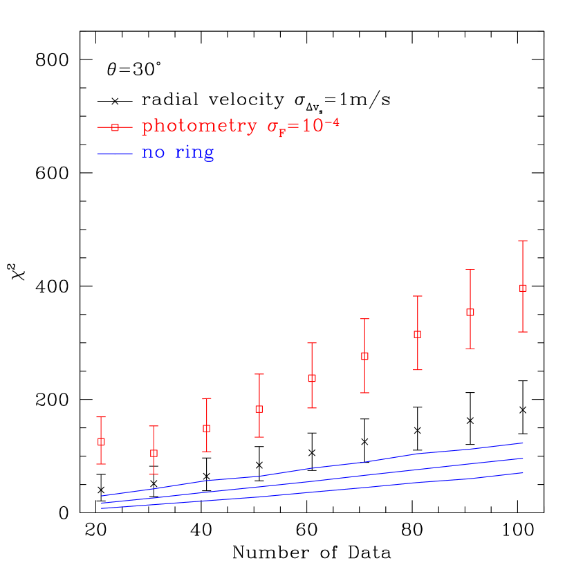
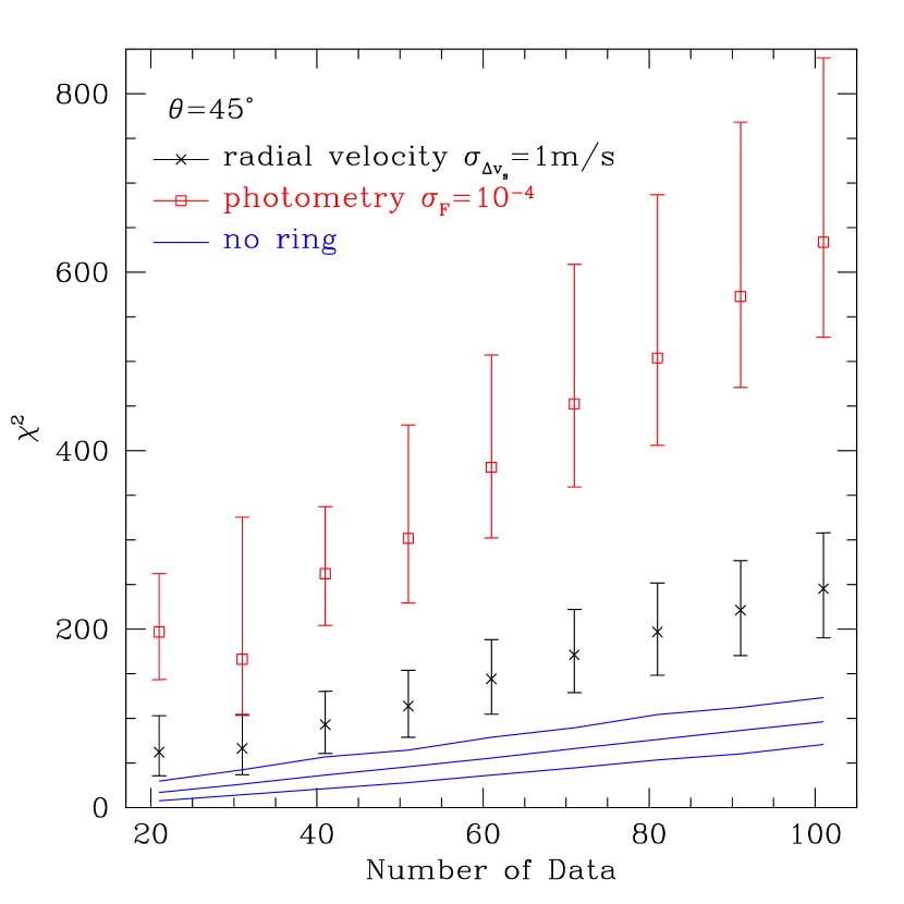
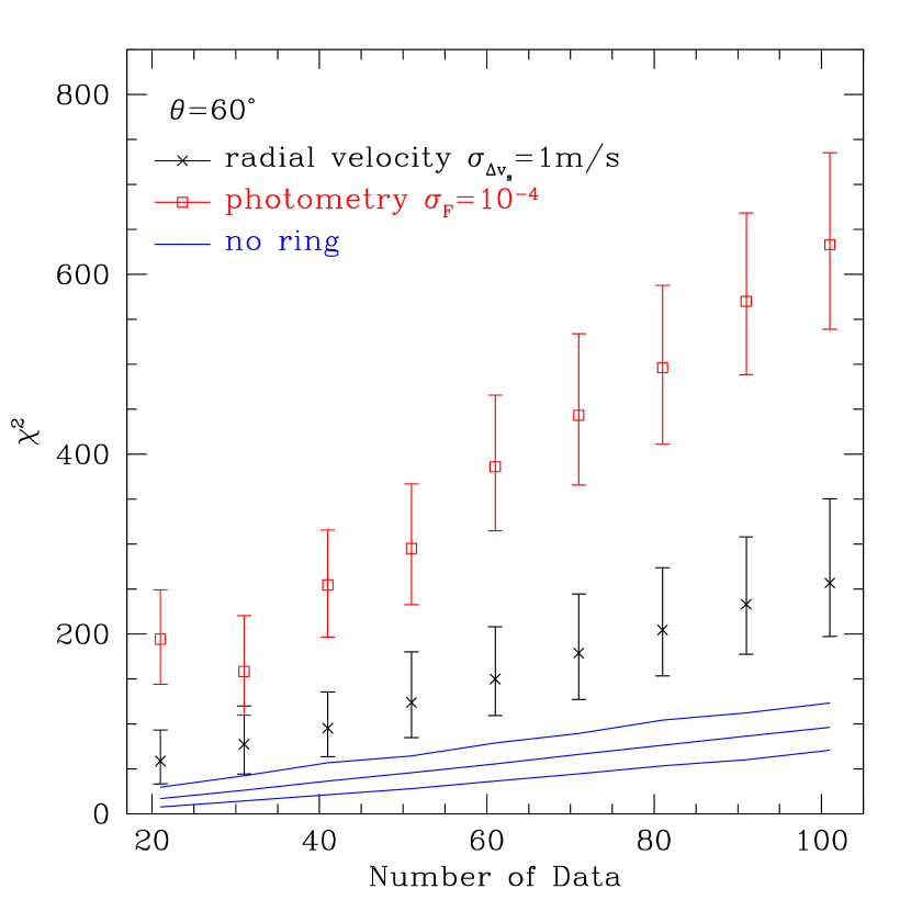
So far we have ignored observational errors of instrumental noises. In this subsection, we discuss the detectability of the ring system and clarify under what conditions the presence of rings is statistically confirmed and is really established as an undisputed fact. For this purpose, we create mock data and measure the residuals of $\Delta v_{s}$ and $F$. Using 1,000 mock realizations, the statistical significance of the residuals is estimated.

We define

$$\chi^{2}=\sum_{i=1}^{N_{\mathcal{O}}}\left[\frac{\mbox{Res}[\mathcal{O}_{i}]}{\sigma_{\mathcal{O}}}\right]^{2}$$ (46)

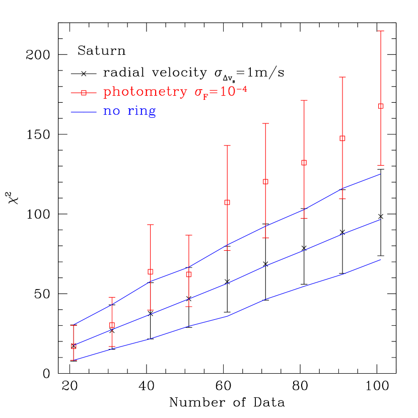
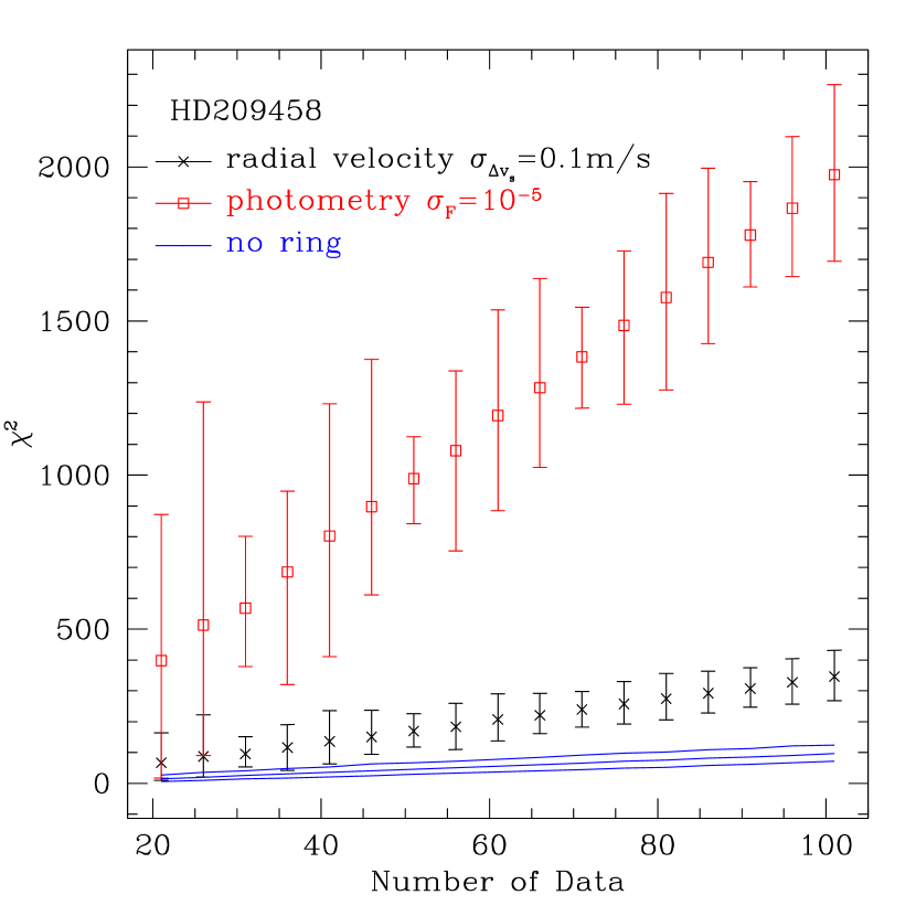
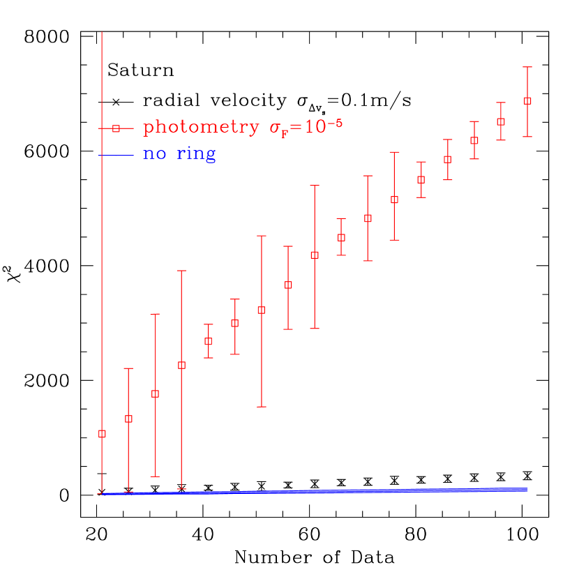
with the subscript $i$ stands for the sample point. Here, the quantity ${\mathcal{O}}$ denotes either $\Delta v_{s}$ or $F$; $\sigma_{\Delta v_{s}}$ and $\sigma_{F}$ are the statistical errors of radial velocity anomaly and relative flux ratio, respectively. We specifically assign the errors of $\sigma_{\Delta v_{s}}=1$ m s^-1 and $\sigma_{F}=10^{-4}$ as currently achieved precision levels, and also of $\sigma_{\Delta v_{s}}=0.1$ m s^-1 and $\sigma_{F}=10^{-5}$ as future precision. The mock data are then created adopting the central values of the fiducial model in Table 1 with Gaussian random errors of $\sigma_{\Delta v_{s}}$ and $\sigma_{F}$.

In Figure 8, we estimate $\chi^{2}$ from 1,000 mock realizations and quantify the scatter of the $\chi^{2}$ functions by varying the number of data samples and the ring parameters of mock data. Basically, we choose the central transiting time as the origin of the time and sample the data at regular interval. For the cases with future precision (bottom panels of Fig.9), however, we shift the origin of the binning randomly within one bin size with respect to the central transiting time. We then explore the effects of bin size by varying the number of data points and computing $\chi^{2}$. If we do not randomly shift the origin of the binning, $\chi^{2}$ shows an artificial oscillation due to the sinusoidal nature of the expected signal, and this becomes prominent for the cases with higher precision. In order to avoid the artificial coherence of the sampled phase, we therefore shift the central position by a size that is randomly chosen between 0 to the size of bin.

Each panel in Figure 8 shows the 95% confidence interval for the distribution of $\chi^{2}$ values around the mean values (open squares for photometric measurements, crosses for spectroscopic measurement). As a reference, we also estimated the scatter of $\chi^{2}$ values from the mock data without rings, and the resulting 95% confidence interval are plotted as solid lines, with middle lines being mean values. Hence, significant deviation from the three reference lines disfavors a ringless planet, suggesting the presence of ring as a plausible solution. In each panel, the mock data were created adopting the fiducial values listed in Table 1, except for the obliquity of ring parameters, $\theta$. We specifically examine the three cases: $\theta=45^{\circ}$ (upper-left), $30^{\circ}$ (upper-right), and $60^{\circ}$ (lower).

Figure 8 indicates that rings with a large obliquity are easily detected. The increased number of both the photometric and spectroscopic samples also improves the detectability, although the photometric data tend to have a better sensitivity compared to the spectroscopic data. This is partly because characterization of the spectroscopic signal requires two additional parameters, i.e., $V\sin I_{s}$ and $\lambda$, in addition to the model parameters of photometric signals. Thus, $\chi^{2}$ values of the spectroscopic measurement are expected to be generally small. Nevertheless, spectroscopic detection/confirmation of rings is valuable and combined data analysis will significantly improve the reliability of the detection. This is especially relevant for planets orbiting around a rapidly rotating star, in which case the spectroscopic signatures of ring during ingress and egress phase become more prominent.

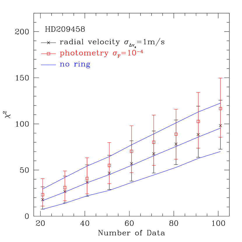
In Figure 9, we also examine the cases for the close-in planet (HD 209458b) assuming a tidally-locked system (left panels) and Saturn system (right panels). The close-in planet is likely to be a tidally-locked system and the obliquity of the ring is thus expected to be rather small in such a case. Thus a possible signature of a ring is inevitably weak and it is difficult to detect with the current sensitivity (Figure 6). On the other hand, Saturn has a relatively large obliquity ($\theta=26.7^{\circ}$) and the photometric signatures of the ring is marginally detectable with the HST photometric accuracy of $10^{-4}$. The spectroscopic signatures are a bit below the detection level of 1 m s^-1 partly because the rotation velocity of the Sun is small ($V\sin I_{s}=1,880$m s^-1).

Nevertheless, the improved precision of future observations will significantly increase the detection threshold. Indeed, the accuracy of spectroscopic measurement is supposed to achieve $\sim$ a few cm s^-1 level (Li et al., 2008; Murphy et al., 2007), and Kepler may reach $\sigma_{\rm F}\approx 10^{-5}$. The lower panels of Figure 9 assume those future precisions. They indicate that if possible systematic effects due to the stellar activity are well under control, the spectroscopic signatures of rings from the ground-based observation are even detectable.

6 Conclusions and discussion

We have explored photometric and spectroscopic detectability of rings around extrasolar transiting planets. We have described a general formulation to predict both the photometric transiting signature in the stellar light curve and the spectroscopic radial velocity anomaly due to the Rossiter effect for a planetary system with a ring. For a face-on ring system, we have provided analytic formulae for those effects, which correspond to an improved version of our previous results (Paper I). We have shown also several numerical results for more general orientations of planetary rings. We found that possible planetary rings around HD 209458b and Saturn may be marginally detectable even with the current observational accuracy as long as sufficiently sampled data points are available. This is very encouraging, and we believe that the detection of rings around extrasolar transiting planets is one of the realistic scientific goals of up-coming space missions.

Figure 8: $\chi^{2}$ with respect to the the best-fit parameters for a ringless planet model against the number of sampled data points (eq.[46]); the mean value of $\chi^{2}$ are plotted in symbols with the error bars indicating the 95% confidence interval estimated from 1,000 mock realizations. Open squares and crosses denote $\chi^{2}$ for photometric data and for spectroscopic data, respectively The mock data were created adopting the fiducial values listed in Table 1, except for the obliquities of the ring axis; $\theta=30^{\circ}$ (upper-left), $45^{\circ}$ (upper-right), and $\theta=60^{\circ}$ (lower). The spectroscopic and photometric accuracies of ($1$ m s^-1, $10^{-4}$) are adopted.

Figure 9: Same as Figure 8, but for HD 209458 and Saturn systems. Left panels show the results for a tidally-locked close-in planet adopting the orbital parameters of HD 209458 system, while right panels are for Saturn system. The model parameters of these examples are described in caption of Figure 6. The upper and lower panels adopt the spectroscopic and photometric accuracies of ($1$ m s^-1, $10^{-4}$) and ($0.1$ m s^-1, $10^{-5}$), respectively.

Let us make a couple of additional comments here. First, our present results may be directly applicable to oblate planets (by setting $\tau=\infty$, $R_{\rm p}=R_{\rm in}=0$, and regarding $R_{\rm out}$ as the surface of the oblate planet, for instance). It would be unlikely that the slow spin velocity of tidally-locked close-in planets significantly distorts their surface, but it would be interesting to put any constraints on the oblateness of the planets (e.g., Seager & Hui, 2002). Second, while one would expect that the planetary spin axis is aligned with the orbital axis, Winn & Holman (2005) argued an interesting possibility that this is not the case. Thus the detection of the ring can test their proposal in a straightforward manner if the planetary spin axis is perpendicular to the ring.

We have to admit, however, that the existence of a Saturnian planet with a ring in extra-solar systems is very speculative, in particular for close-in planets where any interpolation from our Solar system may not be justified. Thus we share the same feeling that Nagaoka expressed more than a hundred years ago even in the historical paper (Nagaoka, 1904): “There are various problems which will possibly be capable of being attacked on the hypothesis of a Saturnian system ”. Nevertheless we cannot resist the temptation to conclude our paper by quoting the last sentence in his paper: “The rough calculation and rather unpolished exposition of various phenomena above sketched may serve as a hint to a more complete solution of atomic structure.”

Finally it would be interesting to note the analogy between the extrasolar planetary system and the atomic model; radial velocity modulation of stars due to planets, the Rossiter effect of transiting planets, and the signature of rings correspond to the atomic orbital angular momentum, the spin of proton, and the spin of electrons. We should not forget that the wild idea of Nagaoka led to quantum physics, which turned out to provide the physical basis of the astronomical spectroscopic observations via the orbital and spin angular momenta of various atomic systems, and therefore he indeed opened a way to the extrasolar planet search.

We thank Joshua Winn, Edwin Turner and Norio Narita for useful discussions, and Erik Reese for a careful reading of the manuscript. We also thank an anonymous referee for several constructive comments which improved the presentation of the earlier manuscript. This work is partially supported by Grants-in-Aid for Scientific Research from the Japan Society for Promotion of Science (No.14102004, 16340053 and 18740132).

Appendix A Approximation of Integrals

Here, we present the approximate expressions for the integrals $W_{i}$ $(i=1$–$4)$ that appear in the formulae (19) and (20). These quantities are all expressed in terms of the planet position $\rho=(X_{p}^{2}+Z_{p}^{2})^{1/2}$ together with the small parameter $\gamma_{\rm ps}\equiv R_{p}/R_{s}$. Before writing down the approximate formulae, we give precise definitions of these integrals (see Sec.5 of Paper I):

$$W_{1} = \frac{1}{\pi R_{p}^{2}}\,\int\!\!\!\int_{S}dxdz\sqrt{1-(x^{2}+z^{2})/R_{s}^{2}},$$ (A1)

$$W_{2} = \frac{1}{X_{p}\,\pi R_{p}^{2}}\,\int\!\!\!\int_{S}dxdz\,\,x\sqrt{1-(x^{2}+z^{2})/R_{s}^{2}},$$ (A2)

$$W_{3} = \int\!\!\!\int_{S^{\prime}}d\tilde{x}d\tilde{z}\sqrt{1-\tilde{x}^{2}-\tilde{z}^{2}},$$ (A3)

$$W_{4} = \int\!\!\!\int_{S^{\prime}}d\tilde{x}d\tilde{z}\,\,\tilde{x}\sqrt{1-\tilde{x}^{2}-\tilde{z}^{2}},$$ (A4)

where the variables $(x,z)$ means the coordinate system defined in Figure 1. The variables $(\tilde{x},\tilde{z})$ are related to the coordinate $(x,z)$ through

$$\left(\begin{array}[]{c}\tilde{x}\\ \tilde{z}\end{array}\right)=\frac{1}{R_{s}\sqrt{X_{p}^{2}+Z_{p}^{2}}}\left(\begin{array}[]{cc}X_{p}&Z_{p}\\ -Z_{p}&X_{p}\end{array}\right)\left(\begin{array}[]{c}x\\ z\end{array}\right).$$ (A11)

Note that the integrals $W_{1}$ and $W_{2}$ are carried out over the entire planetary disk during the complete transit phase, while the regions of the integrals $W_{3}$ and $W_{4}$ are restricted to the overlapped region between planetary and stellar disks during the ingress and the egress phases.

The approximate expressions for the integrals $W_{1}$ and $W_{2}$ are derived by expanding the integrand in powers of $\gamma$. The resultant expressions become

$$W_{1} \simeq (1-\rho^{2})^{1/2}\,\,-\,\,\gamma^{2}\,\frac{2-\rho^{2}}{8(1-\rho^{2})^{3/2}}+{\cal O}(\gamma^{4}).$$ (A12)

$$\ W_{2} \simeq (1-\rho^{2})^{1/2}\,\,-\,\,\gamma^{2}\,\frac{4-3\rho^{2}}{8(1-\rho^{2})^{3/2}}+{\cal O}(\gamma^{4}).$$ (A13)

Consider next the integrals $W_{3}$ and $W_{4}$. They correspond to the ingress and egress phases where $\rho\simeq 1$, and the approximation $1-\rho^{2}\gg\gamma$, which is used in the perturbative expansion for $W_{1}$ and $W_{2}$, breaks down. Thus we attempt to find better approximate expressions as follows. Let us integrate first and rewrite $W_{3}$ and $W_{4}$ as

$$W_{3} = \frac{\pi}{6}(1-x_{0})^{2}(2+x_{0})+\int_{x_{0}+\zeta-\gamma}^{x_{0}}d\tilde{x}~{}g(\tilde{x};\eta_{p},\gamma),$$ (A14)

$$W_{4} = \frac{\pi}{8}(1-x_{0}^{2})^{2}+\int_{x_{0}+\zeta-\gamma}^{x_{0}}d\tilde{x}~{}\tilde{x}g(\tilde{x};\eta_{p},\gamma).$$ (A15)

where the function $g$ is given by

$$g(\tilde{x};\,\eta_{p},\,\gamma) \equiv (1-\tilde{x}^{2})\sin^{-1}\left\{\frac{\gamma^{2}-(\tilde{x}-1-\eta_{p})^{2}}{1-\tilde{x}^{2}}\right\}^{1/2}$$ (A17)

$$\quad\quad\quad+\sqrt{2(1+\eta_{p})(x_{0}-\tilde{x})\{\gamma^{2}-(\tilde{x}-1-\eta_{p})^{2}\}},$$

where

$$x_{0} = 1-\frac{\gamma^{2}-\eta_{p}^{2}}{2(1+\eta_{p})},$$ (A18)

$$\zeta = \frac{2\eta_{p}+\gamma^{2}+\eta_{p}^{2}}{2(1+\eta_{p})}.$$ (A19)

Equations (A14) and (A15) are still too complicated to integrate analytically. Thus we approximate the integrand of equation (A14) as

$$g(\tilde{x};\eta_{p},\gamma)=C_{3}\,\,g(x_{c};\eta_{p},\gamma)\sqrt{\frac{(x_{0}-\tilde{x})(\tilde{x}-x_{0}-\zeta+\gamma)}{(x_{0}-x_{c})(x_{c}-x_{0}-\zeta+\gamma)}},$$ (A20)

where

$$x_{c} = x_{0}+s(\zeta-\gamma).$$ (A21)

In the above equations, we determine the two constants $s$ and $C_{3}$ as follows. From the continuity of the first and second expressions of equation (28), $C_{3}$ is written in terms of $s$:

$$C_{3}=\frac{4\sqrt{s(1-s)}\gamma}{g(1-2s\gamma;-\gamma,\gamma)}W_{1}(1-\gamma).$$ (A22)

The value of $s$ is obtained empirically obtained to yield the best-fit to the numerical results. Here we adopt $s=0.4$ which gives a slightly better fit than $s=0.5$ that was used in Paper I. Finally we obtain

$$W_{3}\simeq\frac{\pi}{6}(1-x_{0})^{2}(2+x_{0})+\frac{\pi}{2}\gamma(\gamma-\zeta)\frac{g(x_{c};\eta_{p},\gamma)}{g(1-2s\gamma;-\gamma,\gamma)}W_{1}(1-\gamma).$$ (A23)

We repeat a similar procedure for equation (A15). In this case, the constant $C_{3}$ is replaced by

$$C_{4}=\frac{4\sqrt{s(1-s)}\gamma}{g(1-2s\gamma;-\gamma,\gamma)}W_{2}(1-\gamma),$$ (A24)

and we adopt $s=0.4$ as above. Then an approximate analytic expression for $W_{4}$ is given as

$$W_{4}\simeq\frac{\pi}{8}(1-x_{0}^{2})^{2}+\frac{\pi}{4}\gamma(\gamma-\zeta)(2x_{0}+\zeta-\gamma)\frac{g(x_{c};\eta_{p},\gamma)}{g(1-2s\gamma;-\gamma,\gamma)}W_{2}(1-\gamma).$$ (A25)

Table 1: List of parameters

Variables	Fiducial value	Meaning
Internal parameters of star
$R_{s}$	1.146$R_{\odot}$	Stellar radius
$u_{1}$	0.2925	Limb darkening parameter
$u_{2}$	0.3475	Limb darkening parameter
$\Omega_{s}$	$R_{s}\Omega_{s}\sin I_{s}=4700\,{\rm m\,s^{-1}}$	Spin rotation velocity of star
$I_{s}$	-	Inclination between stellar spin axis and $y$-axis
Internal parameters of planet and ring
$R_{p}$	1.347$R_{J}$	Planetary radius
$\lambda$	$0^{\circ}$	Angle between $z$-axis
		and normal vector $\hat{{\mbox{\boldmath${n}$}}}_{p}$ on $(x,z)$-plane
$R_{\rm in}$	1.5$R_{p}$	Radius of inner edge of ring
$R_{\rm out}$	2.0$R_{p}$	Radius of outer edge of ring
$\tau$	1.0	Optical depth normal to ring surface
$\theta$	$45^{\circ}$	Obliquity angle of ring axis to $z$ axis
$\phi$	$0^{\circ}$	Azimuthal angle of ring axis around $z$ axis
Orbital parameters
$a$	$3$AU	Semi-major axis
$P_{\rm orbit}$	$1809.01$days	Orbital period
$i_{\rm orbit}$	$90^{\circ}$	Inclination angle between
		normal direction of orbital plane and $y$-axis
$b$	-	Impact parameter, $b=(a/R_{s})\cos i_{\rm orbit}$

References

- Barnes & Fortney (2004) Barnes, J. W., & Fortney, J. J. 2004, ApJ, 616, 1193
- Brown et al. (2001) Brown, T. M., Charbonneau, D., Gilliland, R. L., Noyes, R. W., & Burrows, A. 2001, ApJ, 552, 699
- Charbonneau et al. (2000) Charbonneau, D. et al., 2000, ApJ, 529, L45.
- Colwell et al. (2007) Colwell, J. E., Esposito, L. W., Sremcevic, M., Stewart, G. R., & McClintock, W. E., 2007, Icarus, 190, 127.
- Elliot, Dunham & Mink (1977) Elliot, J.L., Dunham, E.W., & Mink, D.J., 1977, Nature, 267, 328.
- Esposito (2006) Esposito, L., 2006, Planetary Rings (Cambridge University Press, Cambridge)
- Gaudi, Chang & Han (2003) Gaudi, B.S., Chang, H., & Han, C. 2003, ApJ, 586, 527
- Goldreich & Tremaine (1982) Goldreich, P. & Tremaine, S. 1982, ARA&A, 20, 249
- Hosokawa (1953) Hosokawa, Y. 1953, PASJ, 5, 88.
- Hubbard et al. (1977) Hubbard, W.B., Voyens, G.V., Gehrels, T., Smith, B.A., and Zellner, B.H., 1977, Nature, 268, 33.
- Hubbard et al. (1986) Hubbard, W.B., Brahic, A., Sicardy, B., Elicer, L.-R., Roques, F., and Vilas, F., 1986, Nature, 319, 636.
- Kopal (1942) Kopal, Z. 1942, Proc. U.S. Natl. Acad. Sci., 28, 133
- Kopal (1945) Kopal, Z. 1945, Proc. Am. Phil. Soc. 89, 517
- Li et al. (2008) Li, C-H. et al., 2008, Nature, 452, 610
- Lovis et al. (2006) C. Lovis, M. Mayor, F. Pepe, Y. Alibert, W. Benz, F. Bouchy, A. Correia, J. Laskar, C. Mordasini, D. Queloz, N. Santos, S. Udry, J-L. Bertaux, J-P. Sivan, 2006, Nature, 441, 305
- McLaughlin (1924) McLaughlin, D. B. 1924, ApJ, 60, 22
- Murphy et al. (2007) Murphy, M.T. et al., 2007, MNRAS, 380, 839
- Murray & Dermott (1999) Murray, C.D. and Dermott, S.F., 1999, Solar System Dynamics (University of Cambridge Press: Cambridge)
- Nagaoka (1903) Nagaoka, H. 1903, Tokyo Sugaku-Butsurigakukwai Kiji-Gaiyo, 2, 92
- Nagaoka (1904) Nagaoka, H. 1904, Phil.Mag. 7, 445
- Narita et al. (2007) Narita, N., Enya, K., Sato, B., Ohta, Y., Winn, J.N., Suto, Y., Taruya, A., Turner, E.L., Aoki, W., Tamura, M., Yamada, T., & Yoshii, Y., 2007, PASJ, 59, 763
- Ohta, Taruya, & Suto (2005) Ohta, Y., Taruya, A., & Suto, Y., 2005, ApJ, 622, 1118 (Paper I)
- Petrie (1938) Petrie, R. M. 1938, Publ. Dominion Astrophys. Obs., 7, 133
- Pollack et al. (1996) Pollack, J.B., Hubickyj, O., Bodenheimer, P., et al. 1996, Icarus, 124, 62
- Queloz et al. (2000) Queloz, D., Eggenberger, A., Mayor, M., Perrier, C., Beuzit, J.L., Naef, D., Sivan, J.P., and Udry, S., 2000, A&A, 359, L13.
- Rossiter (1924) Rossiter, R. A. 1924, ApJ69, 15.
- Rutherford (1911) Rutherford, E. 1911, Phil.Mag. 21, 669
- Sato et al. (2005) Sato, B. et al. 2005, ApJ, 633, 465
- Seager & Hui (2002) Seager, S. & Hui, L. 2002, ApJ, 574,1004
- Wolf et al. (2006) Wolf, A., Laughlin, G., Henry, G., Fischer, D., Marcy, G., Butler, P., & Vogt, S. 2006, ApJ, submitted
- Winn & Holman (2005) Winn, J. N., & Holman, M. J., 2005, ApJ, 628, L159
- Winn et al. (2006) Winn, J. N., Johnson, J. A., Marcy, G, W., Butler, R. P., Vogt, S. S., Henry, G. W., Roussanova, A., Holman, M.J., Enya, K., Narita, N., Suto, Y., & Turner, E.L., 2006, ApJ, 653, L69
- Winn et al. (2005) Winn, J. N., Noyes, R. W., Holman, M. J., Charbonneau, D. B., et al., 2005, ApJ, 631, 1215
- Winn et al. (2007a) Winn, J. N., Holman, M.J., Henry, G.W., Roussanova, A., Enya, K., Yoshii, Y., Shporer, A., Mazeh, T., Johnson, J.A., Narita, N., & Suto, 2007, AJ, 133, 1828
- Winn et al. (2007b) Winn, J.N., Johnson, J.A., Peek, K.M.G., Marcy, G.W., Bakos, G.A., Enya, K., Narita, N., Suto, Y., Turner, E.L., & Vogt, S.S., 2007, ApJ, 665, 167