The Excursion Set Theory of Halo Mass Functions, Halo Clustering, and Halo Growth

Abstract

I review the excursion set theory with particular attention toward applications to cold dark matter halo formation and growth, halo abundance, and halo clustering. After a brief introduction to notation and conventions, I begin by recounting the heuristic argument leading to the mass function of bound objects given by Press & Schechter. I then review the more formal derivation of the Press-Schechter halo mass function that makes use of excursion sets of the density field. The excursion set formalism is powerful and can be applied to numerous other problems. I review the excursion set formalism for describing both halo clustering and bias and the properties of void regions. As one of the most enduring legacies of the excursion set approach and one of its most common applications, I spend considerable time reviewing the excursion set theory of halo growth. This section of the review culminates with the description of two Monte Carlo methods for generating ensembles of halo mass accretion histories. In the last section, I emphasize that the standard excursion set approach is the result of several simplifying assumptions. Dropping these assumptions can lead to more faithful predictions and open excursion set theory to new applications. One such assumption is that the height of the barriers that define collapsed objects is a constant function of scale. I illustrate the implementation of the excursion set approach for barriers of arbitrary shape. One such application is the now well-known improvement of the excursion set mass function derived from the “moving” barrier for ellipsoidal collapse. I also emphasize that the statement that halo accretion histories are independent of halo environment in the excursion set approach is not a general prediction of the theory. It is a simplifying assumption. I review the method for constructing correlated random walks of the density field in the more general case. I construct a simple toy model to illustrate that excursion set theory (with a constant barrier height) makes a simple and general prediction for the relation between halo accretion histories and the large-scale environments of halos: regions of high density preferentially contain late-forming halos and conversely for regions of low density. I conclude with a brief discussion of the importance of this prediction relative to recent numerical studies of the environmental dependence of halo properties.

I Introduction

In the standard, hierarchical, cold dark matter (CDM) paradigm of cosmological structure formation, galaxy formation begins with the gravitational collapse of overdense regions into bound, virialized halos of dark matter (DM). The average density of dark matter outweighs that of baryonic matter by roughly six to one. Bound in the potential wells of dark matter halos, baryons proceed to cool, condense, and form galaxies. Understanding the fundamental properties and abundances of these dark matter halos is the first, necessary step in understanding the properties of galaxies.

In this manuscript, I review the excursion set (also referred to as “extended Press-Schechter”) approach to dark matter halo formation and halo clustering. I begin with some preliminaries that serve to define my notation and several common conventions in § II. I review the heuristic argument that Press & Schechter Press and Schechter (1974) used to derive their analytic mass function in § III. In this section I also draw attention to the most obvious weakness of the Press-Schechter argument, often referred to as the cloud-in-cloud problem. In § IV I review the theory of excursion sets of the density contrast field and the manner in which the excursion set theory solves the cloud-in-cloud problem. The standard excursion set theory then yields a halo mass function identical to the Press-Schechter proposal.

The excursion set approach is very powerful and yields a great deal of insight into numerous aspects of halo formation and halo clustering. Following the mass function, one of the most immediate applications of the excursion set approach is to predict the clustering properties of dark matter halos relative to the dark matter. I review the issue of halo bias in the context of the excursion set theory in § V. The bias relation derived in § V was derived prior to widespread use of excursion set theory, but this section also partially serves as a warm-up for the more complex arguments that follow. In § VI, I summarize the excursion set theory of the void population. The content of § V and § VI contain some redundant information, but my intention is that repetition of the basic arguments in these sections will reinforce the logic and methods of the excursion set approach.

In § VII, I review excursion set predictions for halo conditional mass functions, halo accretion rates, and halo formation times. The culmination of this review is the predominant algorithm for generating Monte Carlo merger histories on a halo-by-halo basis using the excursion set theory. This algorithm, refined most recently by Somerville & Kolatt Somerville and Kolatt (1999) and Cole et al. Cole et al. (2000) to similar effect, is the subject of § VIII.

Recent advancement in both theoretical methods and observational data have emphasized the weaknesses of the simplest implementation of the excursion set model. Nevertheless, the basic idea of the excursion set model is extremely valuable because it provides a toolbox for making quick estimates for numerous halo and galaxy properties. In addition, and perhaps more importantly, the excursion set approach remains one of the principle frameworks for qualitative reasoning and understanding of the complex results of direct, cosmological, numerical simulations. The algorithm for generating merger trees is one of the most widely used aspects of excursion set theory and is likely to remain one of the primary legacies of excursion set theory. These excursion set halo merger trees form the basis of countless semi-analytic explorations of the physical processes involved in galaxy formation (examples are Refs. Somerville and Primack (1999); Cole et al. (2000); Kauffmann and Haehnelt (2000)). The excursion set halo merger trees are considerably less costly to produce than direct $N$-body simulation, so they continue to be used to make general points (there are many examples, but an elegant recent example is Ref. Neistein et al. (2006)) and to study the effects of varying cosmological parameters (e.g., Ref. Zentner and Bullock (2003)). Moreover, excursion set merger histories are also the basis of many models that aim to expand upon simulation results, either by extending results beyond the resolution of current simulations or building statistically-large halo samples in regimes where simulations have not, by modeling nonlinear dynamics in simplified ways (e.g., Refs. Zentner and Bullock (2003); Benson et al. (2004); Koushiappas et al. (2004); Zentner et al. (2005); Peñarrubia and Benson (2005); Taylor and Babul (2005a, b)).

The simplest implementation of the excursion set theory, which is the primary focus of these lectures, is certainly not the only possible implementation of the excursion set approach. Excursion set theory can be modified to approximate numerous physical effects that are ignored in the derivations of the most basic set of equations. I address extensions of the excursion set models and proposed improvements in the final section of this review, § IX. This section highlights areas where excursion set theory can be expanded and points toward the principle references where these extensions have been developed. I focus primarily on generalized forms for the barrier shape and excursion sets of correlated random walks. An interesting aspect of this section is the calculation of a general excursion set prediction for the dependence of halo formation times on the large-scale environments of halos. I close with a mention of the PINOCCHIO algorithm, developed by P. Monaco and collaborators primarily in Refs. Monaco et al. (2002a, b); Taffoni et al. (2002), which makes use of Lagrangian perturbation theory together with some of the ideas of the excursion set approach to produce, of many things, halo merger histories.

My primary aims are to present a relatively concise, pedagogical review of the basic logic and techniques of excursion set theory that can be used as a springboard to new studies and to collect the most important results of excursion set theory into a single manuscript, with a single notation. As such, the reference list contained in this manuscript is by no means an exhaustive review of the literature on analytic halo formation or even the excursion set approach. Many important contributions have been omitted in the interest of brevity and to limit the scope of the lectures. However, the references should be sufficient to develop the fundamental logic of the excursion set approach and the basic tools needed to extend this approach to new problems. As a minimal approach, the basic development of the excursion set approach can be followed through the series of papers by Bardeen et al. Bardeen et al. (1986), Bond et al. Bond et al. (1991), Lacey & Cole Lacey and Cole (1993, 1994), Sheth & Lemson Sheth and Lemson (1999), and Somerville & Kolatt Somerville and Kolatt (1999). The various manuscripts contained in the collection edited by Wax Wax (1954) are an extremely valuable resource for understanding stochastic processes and deriving many of the basic results of excursion set theory (including results not contained in this review). Of the articles reprinted in the Wax collection, those by Chandrasekhar Chandrasekhar (1943), and Rice Rice (1944, 1945) are probably of the most immediate interest.

II Notation and Conventions

In the following, I consider fluctuations in the density field $\rho(\vec{x})$ described by the density contrast $\delta(\vec{x})\equiv[\rho(\vec{x})-\rho_{\mathrm{M}}]/\rho_{\mathrm{M}}$, where $\rho_{\mathrm{M}}$ is the mean mass density in the universe and $\vec{x}$ is a comoving spatial coordinate. In the standard paradigm, the universe is endowed with primordial density fluctuations during an epoch of cosmological inflation and the primordial density contrast is a statistically homogeneous and isotropic Gaussian random field. This means that the joint probability distribution of the density contrast at a set of points in space is given by a multivariate Gaussian distribution. Homogeneity requires that the mean $\langle\delta(\vec{x})\rangle$, of the distribution and the two-point function $\langle\delta(\vec{x}_{1})\delta(\vec{x}_{2})\rangle\equiv\xi(\vec{x}_{1},\vec{x}_{2})$ be invariant under translations. The two-point function is then a function only of the separation vector between two points, $\xi(\vec{x}_{1},\vec{x}_{2})=\xi(\vec{x}_{1}-\vec{x}_{2})$. Isotropy requires that $\xi(\vec{x})$ is invariant under rotations as well, so the two-point correlation function is only a function of the distance between two points, $\xi(\vec{x}_{1},\vec{x}_{2})=\xi(|\vec{x}_{1}-\vec{x}_{2}|)$.

The Fourier transform of the density contrast is given by the convention

$$\delta(\vec{k})=\int\mathrm{d}^{3}x\ \delta(\vec{x})e^{i\vec{k}\cdot\vec{x}}$$ (1)

with the inverse transform

$$\delta(\vec{x})=\frac{1}{(2\pi)^{3}}\int\mathrm{d}^{3}k\ \delta(\vec{k})e^{-i\vec{k}\cdot\vec{x}}.$$ (2)

Notice that the $\delta(\vec{k})$ have dimensions of volume and that for a real-valued field $\delta(\vec{x})$, the Fourier coefficients obey the relation $\delta(-\vec{k})=\delta^{*}(\vec{k})$. We have implicitly assumed that there is some very large cut-off scale $L\equiv V^{1/3}$ that renders the integral $\int|\delta(\vec{x})|\mathrm{d}^{3}x$ finite and that this scale is much larger than any other scale of interest so that it plays no meaningful role. Using these conventions, one can compute the two-point function $\xi(\vec{r})\equiv\langle\delta(\vec{x})\delta(\vec{x}+\vec{r})\rangle$ in terms of the Fourier coefficients, where the average is taken over all space. The two-point function is a function only of the amplitude of $\vec{r}$ due to isotropy, and the result is

$$\xi(r)=\frac{1}{2\pi^{2}}\int k^{3}V^{-1}|\delta(k)|^{2}\ \frac{\sin(kr)}{kr}\ \mathrm{d}\ln k.$$ (3)

The correlation function is the Fourier transform of the power spectrum

$$P(k)\equiv V^{-1}\langle|\delta(k)|^{2}\rangle,$$ (4)

where the average is over an ensemble of universes with the same statistical properties. The power spectrum has dimensions of volume and so a quantity that lends itself more easily to direct interpretation is the dimensionless combination

$$\Delta^{2}(k)\equiv k^{3}P(k)/2\pi^{2}.$$ (5)

The correlation function $\langle\delta^{2}({\vec{x}})\rangle$ is simply the mass variance. From Eq. (3), $\Delta^{2}(k)$ is the contribution to the mass variance from modes in a logarithmic interval in wavenumber, so that $\Delta^{2}(k)\sim 1$ indicates order unity fluctuations in density on scales of order $\sim k$.

In the standard, cold dark matter (CDM) model, $\Delta^{2}(k)$ increases with wavenumber (at least until some exceedingly small scale determined by the physics of the production of the CDM in the early universe), but we observe the density field smoothed with some resolution. Therefore, a quantity of physical interest is the density field smoothed on a particular scale $R_{\mathrm{W}}$,

$$\delta(\vec{x};R_{\mathrm{W}})\equiv\int\mathrm{d}^{3}x^{\prime}\ W(|\vec{x}^{\prime}-\vec{x}|;R_{\mathrm{W}})\delta(\vec{x}^{\prime})$$ (6)

The function $W(x;R_{\mathrm{W}})$ is the window function that weights the density field in a manner that is relevant for the particular application. According to the convention used in Eq. (6), the window function (sometimes called filter function) has units of inverse volume by dimensional arguments. It is also useful to think of a window as having a particular window volume $V_{\mathrm{W}}$. The window volume can be obtained operationally by normalizing $W(x)$ such that it has a maximum value of unity and is dimensionless. Call this new dimensionless window function $W^{\prime}(x)$. The volume is given by integrating to give $V_{\mathrm{W}}=\int\mathrm{d}^{3}xW^{\prime}(x)$. In this way, one thinks of the window weighting points in the space by different amounts. It should be clear that $W(x)=W^{\prime}(x)/V_{\mathrm{W}}$. Roughly speaking, the smoothed field is the average of the density fluctuation in a region of volume $V_{\mathrm{W}}\sim R_{\mathrm{W}}^{3}$. The Fourier transform of the smoothed field is

$$\delta(\vec{k};R_{\mathrm{W}})\equiv W(\vec{k};R_{\mathrm{W}})\delta(\vec{k}),$$ (7)

where $W(\vec{k};R_{\mathrm{W}})$ is the Fourier transform of the window function.

The most natural choice of window function is probably a simple sphere in real space. The window function is then

$$W(x;R_{\mathrm{W}})=\begin{array}[]{lr}\frac{3}{4\pi R_{\mathrm{W}}^{3}}&\mbox{($x\leq R_{\mathrm{W}}$)}\\ 0&\mbox{($x>R_{\mathrm{W}}$)}\end{array}.$$ (8)

In this case, the smoothed field is the average density in spheres of radius $R_{\mathrm{W}}$ about point $\vec{x}$. The window volume is simply $V_{\mathrm{W}}=4\pi R_{\mathrm{W}}^{3}/3$. However, this choice of window has the undesirable property that the sharp transition in configuration space leads to power on all scales in Fourier space. Therefore, it is often convenient to smooth the boundary in real space. As I discuss below, it is often convenient to introduce particular window functions to ensure that the smoothed field has particular properties. The three most commonly used window functions are the real-space tophat window of Eq. (8), with Fourier transform

$$W(k;R_{\mathrm{W}})=\frac{3[\sin(kRR_{\mathrm{W}})-kR_{\mathrm{W}}\cos(kR_{\mathrm{W}})]}{(kR_{\mathrm{W}})^{3}},$$ (9)

the Fourier-space tophat window, and the Gaussian window. The Fourier-space tophat is defined in Fourier space as

$$W(k;R_{\mathrm{W}})=\begin{array}[]{lr}1&\mbox{($k\leq R_{\mathrm{W}}^{-1}$)}\\ 0&\mbox{($k>R_{\mathrm{W}}^{-1}$)}\end{array},$$ (10)

and is

$$W(x;R_{\mathrm{W}})=\frac{1}{2\pi^{2}R_{\mathrm{W}}^{3}}\frac{(\sin(xR_{\mathrm{W}}^{-1})-xR_{\mathrm{W}}^{-1}\cos(xR_{\mathrm{W}}^{-1}))}{(xR_{\mathrm{W}}^{-1})^{3}}$$ (11)

in real space. A disadvantage of this window is that it does not have a well-defined volume. This concern creeps up repeatedly in what follows. The Gaussian window is

$$W(x;R_{\mathrm{W}})=\frac{\exp(-x^{2}/2R_{\mathrm{W}}^{2})}{(2\pi)^{3/2}R_{\mathrm{W}}^{3}}$$ (12)

with a Fourier transform that also has the form of a Gaussian

$$W(k;R_{\mathrm{W}})=\exp(-k^{2}/2R_{\mathrm{W}}^{-2}),$$ (13)

with a width that is the reciprocal of its width in real space. The volume of the Gaussian window is $V_{\mathrm{W}}=(2\pi)^{3/2}R_{\mathrm{W}}^{3}$.

The density fluctuation field is assumed to be a Gaussian random variable so the smoothed density fluctuation field $\delta(\vec{x};R)$ is then a Gaussian random variable as well because it represents a sum of Gaussian random variables. The variance of $\delta(\vec{x};R)$ can be computed in the same way as before [see Eq. (3)] and is

$$\sigma^{2}(R)=\langle\delta^{2}(\vec{x};R)\rangle=\int\mathrm{d}\ln k\ \Delta^{2}(k)|W(k;R)|^{2}.$$ (14)

Thus, the probability of attaining a value of $\delta(\vec{x};R)$ between $\delta$ and $\delta+\mathrm{d}\delta$ is

$$P(\delta;R)\mathrm{d}\delta=\frac{1}{\sqrt{2\pi\sigma^{2}(R)}}\exp[-\delta^{2}/2\sigma^{2}(R)]\mathrm{d}\delta.$$ (15)

It is common to refer to the smoothing scale as either a length, as above, or a mass given by the mean density multiplied by the volume of the window $M=\rho_{\mathrm{M}}V_{\mathrm{W}}$. The left panel of Fig. 1 depicts a standard model power spectrum expressed as the variance of the smoothed density field, smoothed with a real-space tophat, and shows the smoothing scale in terms of both mass and length. The right panel of Fig. 1 shows the rms density fluctuation per logarithmic interval in wavenumber $\Delta(k)$. The power spectra were computed assuming $\Omega_{\mathrm{M}}=1-\Omega_{\mathrm{\Lambda}}=0.3$, $h=0.7$, $\sigma_{8}=0.93$, $\Omega_{\mathrm{B}}h^{2}=0.022$, and a spectrum of primordial fluctuations with $P_{\mathrm{prim}}(k)\propto k$. I have used the transfer function of Eisenstein & Hu Eisenstein and Hu (1999) to process the scale-invariant primordial spectrum into the post-recombination spectrum of density fluctuations out of which nonlinear structures form.

Figure 1: Power spectra in the standard $\Lambda$CDM cosmology with $\Omega_{\mathrm{M}}=1-\Omega_{\mathrm{\Lambda}}=0.3$, $h=0.7$, $\sigma_{8}=0.93$, and $\Omega_{\mathrm{B}}h^{2}=0.022$. The left panel shows the mass variance smoothed with a real space tophat window as a function of the smoothing mass or smoothing radius [Eq. (14)]. The right panel shows the rms density fluctuation per logarithmic interval of wavenumber as a function of wavenumber [Eq. (3)].

III The Press-Schechter Mass Function

Press & Schechter Press and Schechter (1974) derived a relation for the mass spectrum of virialized objects from the hierarchical density field. In hierarchical models, there is structure on all scales and the variance $\sigma^{2}(R)\rightarrow\infty$ as the smoothing scale $R\rightarrow 0$. Press & Schechter essentially assumed that objects will collapse on some small scale once the smoothed density contrast on this scale exceeds some threshold value, but that the nonlinearities introduced by these virialized objects do not affect the collapse of overdense regions on much larger scales. The collapsed objects act only as resolution elements that trace the larger-scale fluctuations which may collapse at some later time. Strictly speaking, this is not correct; however, it is approximately true when primordial power spectra are sufficiently shallow that the additional large-scale power generated by nonlinearities is small compared to the primordial fluctuations on these scales (a study in one-dimension is Ref. Williams et al. (1991)). Moreover, this assumption leads to a simple parsing of the ingredients in the formation of nonlinear structure. The first ingredient is a characterization of the statistical properties of the primordial density fluctuations. In the standard picture this is set during the inflationary epoch. The second ingredient is the evolution of overdensities according to linear perturbation theory. This is encapsulated in the growth function $D(a)=\delta(k,a)/\delta(k,a=1)$ which is specified by the evolution of the background cosmology (e.g., Refs. Carroll et al. (1992); Bildhauer et al. (1992); Lacey and Cole (1993)). The last ingredient is the threshold for collapse into a virialized object and is determined by examining the nonlinear collapse of spherical overdensities.

Press & Schechter stated that the likelihood for collapse of objects of a specific size or mass ($R\propto M^{1/3}$) could be computed by examining the density fluctuations on the desired scale. They continued by using a model for the collapse of a spherical tophat overdensity to argue that collapse on scale $R$ should occur roughly when the smoothed density on that scale exceeds a critical value $\delta_{\mathrm{c}}$, of order unity, independent of $R$.

The implementation of the Press-Schechter prescription is simple. The mass within a region in which the smoothed density fluctuation (dictated by the linear theory) is the critical value $\delta_{\mathrm{c}}$, at some redshift $z$, corresponds to an object that has just virialized with mass $M(R)$. The relationship between mass and smoothing scale is set by the volume of the window function. As an example, the relationship is $M=4\pi\rho_{\mathrm{M}}R^{3}/3$ for a tophat window and $M=(2\pi)^{3/2}\rho_{\mathrm{M}}R^{3}$ for a Gaussian window. Further, any region that exceeds the critical density fluctuation threshold, will meet that threshold when smoothed on some larger scale $R^{\prime}>R$. Consequently, the cumulative probability for a region to have a smoothed density above threshold gives the fractional volume occupied by virialized objects larger than the smoothing scale $F(M)$. Integrating Eq. (15), this probability is

$$F(M)=\int_{\delta_{\mathrm{c}}}^{\infty}P(\delta;R)\mathrm{d}\delta=\frac{1}{2}\mathrm{erfc}\Bigg{(}\frac{\nu}{\sqrt{2}}\Bigg{)},$$ (16)

where $\mathrm{erfc}(x)$ is the complementary error function, and $\nu\equiv\delta_{\mathrm{c}}/\sigma(M)$ is the height of the threshold in units of the standard deviation of the smoothed density distribution. In this model, collapse of mass $M$ is defined so that it occurs when the smoothed density fluctuation is $\delta_{\mathrm{c}}$ on the appropriate scale. Thus there is a typical scale that is collapsing at the present epoch, $M_{\star}$, when the variance is $\sigma(M_{\star})=\delta_{\mathrm{c}}$.

In the hierarchical power spectra that we consider, $\sigma(R)$ becomes arbitrarily large as $R$ becomes arbitrarily small. Thus, $F(0)$ in Eq. (16) should give the fraction of all mass in virialized objects; however, $\mathrm{erfc}(0)=1$ so that Eq. (16) states that only half of the mass density of the universe is contained in virialized objects. Press & Schechter noted this as a problem associated with not counting underdense regions in the integral Eq. (16). These authors argued that underdense regions will collapse onto overdense regions and multiplied $F(M)$ in Eq. (16) by a factor of two in order to account for all mass. Though the sense of this effect is certainly such that more mass will be contained in bound objects, that this should lead to precisely a factor of two increase in $F(M)$ is far from convincing.

Proceeding with this extra factor of two, the number of virialized objects with masses between $M$ and $M+\mathrm{d}M$ is

$$\frac{\mathrm{d}n}{\mathrm{d}M}\mathrm{d}M=\frac{\rho_{\mathrm{M}}}{M}\Bigg{|}\frac{\mathrm{d}F(M)}{\mathrm{d}M}\Bigg{|}\mathrm{d}M.$$ (17)

In terms of the mass variance, this is

$$\frac{\mathrm{d}n}{\mathrm{d}M}\ \mathrm{d}M = \sqrt{\frac{2}{\pi}}\frac{\rho_{\mathrm{M}}}{M^{2}}\frac{\delta_{\mathrm{c}}}{\sigma}\Bigg{|}\frac{\mathrm{d}\ln\sigma}{\mathrm{d}\ln M}\Bigg{|}\exp\Bigg{(}-\frac{\delta_{\mathrm{c}}^{2}}{2\sigma^{2}}\Bigg{)}\ \mathrm{d}M$$ (18)

$$= \sqrt{\frac{2}{\pi}}\frac{\rho_{\mathrm{M}}}{M^{2}}\ \nu\frac{\mathrm{d}\ln\nu}{\mathrm{d}\ln M}\ \exp\Bigg{(}-\frac{\nu^{2}}{2}\Bigg{)}\ \mathrm{d}M.$$

Without regard to the details of the shape of the power spectrum, $\sigma(M)$ or $\nu(M)$, the mass function is close to a power law $\mathrm{d}n/\mathrm{d}M\propto M^{-2}$ for $M\ll M_{\star}$ and is exponentially cut-off for $M\lower 2.58334pt\vbox{\hbox{$\buildrel\textstyle>\over{\sim}\ $}}M_{\star}$.

IV Excursion Set Theory of the Mass Function

A weakness of the Press-Schechter approach is that it does not account for the fact that at a particular smoothing scale $\delta(\vec{x};R)$ may be less than $\delta_{\mathrm{c}}$, yet it may be larger than $\delta_{\mathrm{c}}$ at some larger smoothing scale $R^{\prime}>R$. It seems natural that this larger volume should collapse to form a virialized object, overwhelming the more diffuse patches within it. Clearly, the sense of including this effect is to increase the fraction of mass in collapsed objects and mitigate the factor of two discrepancy in the Press-Schechter formulas. In the literature, the issue of regions below threshold on a particular scale, but above threshold on a larger scale is referred to as the “cloud-in-cloud” problem. The cloud-in-cloud problem is closely tied to the Press-Schechter factor of two as I discuss below.

To solve the cloud-in-cloud problem, it is necessary to compute the largest value of the smoothing scale for which the density threshold is exceeded. This was done in a formal way by Bond et al. Bond et al. (1991) (see also Refs. Epstein (1983); Peacock and Heavens (1990); Bower (1991)) and I follow their approach quite closely. The development of Bond et al. in turn follows closely the elegant review of stochastic processes by Chandrasekhar Chandrasekhar (1943), and makes use of results from both Ref. Rice (1944) and Ref. Adler (1981).

In what follows, I consider the density contrast field evaluated at some early time far before any scales of interest have approached the nonlinear regime, but extrapolated to the present day using linear perturbation theory. In this way, the density contrast field does not need to obey the physical constraint $\delta\geq-1$ because this is merely the linear extrapolation of a density contrast of much smaller magnitude. In addition, all coordinates are Lagrangian coordinates defined at the same early time so that the position of each mass element is independent of time. The excursion set theory is, at its foundation, a set of rules for assigning mass elements to virialized objects of various sizes. Where needed, I will introduce the necessary conversions that map the initial Lagrangian sizes of overdense and underdense regions onto Eulerian coordinates, thereby accounting for the contraction or expansion of such regions respectively.

Consider again evaluating the field $\delta(\vec{x};R)$ at various values of the smoothing scale $R$, at a single point $\vec{x}$. For now, I will suppress the argument $\vec{x}$ and consider $\delta(R)$ as a function of smoothing scale at a single point in space. For very large $R$, $\sigma(R)\ll\delta_{\mathrm{c}}$ so the probability that the region lies above the boundary $\delta_{\mathrm{c}}$ is vanishingly small. With decreasing $R$, the standard deviation becomes larger and $\delta(R)$ will eventually reach $\delta_{\mathrm{c}}$ at the first up-crossing of the boundary. The problem is to compute the probability that the first up-crossing of the barrier at $\delta_{\mathrm{c}}$ occurs on a scale $R$. For simplicity in what follows, let $S\equiv\sigma^{2}(R)$ and let the value of $S$ serve to denote the smoothing scale by exploiting the fact that $S$ is a monotonically decreasing function of $R$. I will then refer to the density contrast on that scale as $\delta(S)$. Throughout this discussion, it is important to remember that increasing $S$ corresponds to decreasing $R$. The problem is to compute the probability that the first up-crossing through the barrier occurs between a value $S$ and $S+\mathrm{d}S$.

Consider starting at a large smoothing scale, or small $S=S_{1}$, where $\delta(S_{1})\equiv\delta_{1}<\delta_{\mathrm{c}}$. For a given change in the filtering scale $\Delta S$, there is some distribution for the probability of reaching $\delta_{2}$ after an increment $\Delta S=S_{2}-S_{1}>0$. In general, this probability distribution may depend not only on the size of the step $\Delta S$, but the value of the density field on other scales. If the probability distribution for $\delta_{2}$ after an increment $\Delta S$ depends upon other points on the curve $\delta(S)$, solving for the probability distribution of $\delta$ at a given $S$ is nontrivial. An important special case is when the smoothing window used to define $\delta(S)$ is a k-space tophat as in Eqs. (10)-(11). In that case, increasing the filter scale corresponds to adding a set of independent Fourier modes to the smoothed density. These modes have not played a role in determining $\delta(S)$ at other smoothing scales. In this special case, the transition probability for a change in density $\Delta\delta$ associated with a change in filtering scale $\Delta S$ is Gaussian with zero mean and variance $S_{2}-S_{1}=\Delta S$, independent of the starting point $\delta_{1}(S_{1})$.

Following Bond et al. Bond et al. (1991), it is common to refer to a sequence of $\delta(S_{\mathrm{i}})$ given by many subsequent increases of the smoothing scale by increments $\Delta S_{\mathrm{i}}$ as a trajectory for $\delta(S)$. In the case of k-space tophat filtering of the density field, each trajectory of $\delta(S)$ executes a Brownian random walk. Three examples of such uncorrelated random walks are shown in Fig. 2. Notice that trajectories pierce the “barrier” at $\delta_{\mathrm{c}}$ many times and drop below $\delta_{\mathrm{c}}$ between subsequent up-crossings. The aim of the excursion set approach is to solve the cloud-in-cloud problem by determining the largest smoothing scale $R$ or $M$, or equivalently the smallest value of the variance $S$, at which a trajectory penetrates the barrier at $\delta_{\mathrm{c}}$.

Figure 2: Three examples of random walks of $\delta(S)$ assuming each s step is independent as in the case of a sharp k-space window function. The axes are arbitrary. The horizontal dotted line represents some threshold value $\delta_{\mathrm{c}}$. Notice that trajectories may penetrate the “barrier” at $\delta_{\mathrm{c}}$ many times.

In the case of k-space tophat filtering, the probability of a transition from $\delta_{1}$ to $\delta_{2}=\delta_{1}+\Delta\delta$ is

$$\Pi(\delta_{2},S_{2})\ \mathrm{d}\delta_{2}=\Psi(\Delta\delta;\Delta S)\ \mathrm{d}(\Delta\delta),$$ (19)

where

$$\Psi(\Delta\delta;\Delta S)\ \mathrm{d}(\Delta\delta)=\frac{1}{\sqrt{2\pi\Delta S}}\exp\Bigg{(}-\frac{(\Delta\delta)^{2}}{2(\Delta S)^{2}}\Bigg{)}\ \mathrm{d}(\Delta\delta)$$ (20)

is the Gaussian transition probability. Taking $S_{1}=0$, $S_{2}$ the smoothing scale of interest, and finding the probability of $\delta_{2}\geq\delta_{\mathrm{c}}$ returns the Press-Schechter probability for being in a collapsed object. The fact that some regions will exceed $\delta_{\mathrm{c}}$ for a smaller change in $S$ and then fall below $\delta_{\mathrm{c}}$ by $\Delta S$ has not yet been accounted for.

Consider now, relating the distribution of $\delta$ at one value of the smoothing scale $\Pi(\delta,S)$ to the distribution on a subsequent step $\Pi(\delta,S+\Delta S)$ (smaller smoothing scale, larger $S$). This is

$$\Pi(\delta,S+\Delta S)=\int\mathrm{d}(\Delta\delta)\ \Psi(\Delta\delta;\Delta S)\Pi(\delta-\Delta\delta,S).$$ (21)

Taylor expanding Eq. (21) for small transitions, keeping terms up to $(\Delta\delta^{2})$, and integrating each term yields

$$\frac{\partial\Pi}{\partial S}=\lim_{\Delta S\to 0}\Bigg{(}\frac{\langle(\Delta\delta)^{2}\rangle}{2\Delta S}\frac{\partial^{2}\Pi}{\partial\delta^{2}}-\frac{\langle\Delta\delta\rangle}{\Delta S}\frac{\partial\Pi}{\partial\delta}\Bigg{)}.$$ (22)

Using the fact that the transition probability is a Gaussian with $\langle\Delta\delta\rangle=0$ and $\langle(\Delta\delta)^{2}\rangle=\Delta S$ reveals

$$\frac{\partial\Pi}{\partial S}=\frac{1}{2}\frac{\partial^{2}\Pi}{\partial\delta^{2}}$$ (23)

as the relation governing the evolution of the probability distribution $\Pi$ with smoothing scale. The probability distribution $\Pi$ for trajectories $\delta(S)$ that never exceed $\delta_{\mathrm{c}}$ prior to some specific value of $S$ can be obtained by solving Eq. (23) with the appropriate boundary conditions. The first boundary condition is that $\Pi(\delta,S)$ is finite as $\delta\to-\infty$. Imagining each trajectory as absorbed and removed from the sample of trajectories at the moment it first crosses the threshold at $\delta_{\mathrm{c}}$, then $\Pi(\delta_{\mathrm{c}},S)=0$ provides the second boundary condition.

Eq. (23) may have a familiar form as it is also an equation describing diffusion with no drift or a one-dimensional heat equation describing heat flow in a long, thin, semi-infinite bar. The boundary condition at $\delta=\delta_{\mathrm{c}}$ is analogous to fixing the temperature to zero at this end of the bar. Take $\delta(S_{0})=\delta_{0}$ as an arbitrary starting point for the random walk trajectories so that the initial condition is $\Pi(\delta_{0},S_{0})=\delta_{\mathrm{D}}(\delta_{0})$ where $\delta_{\mathrm{D}}(x)$ is the Dirac delta function. Eq. (23) can now be solved using familiar techniques. It is easiest to work in a shifted variable $\gamma\equiv\delta_{\mathrm{c}}-\delta$ so that the finite boundary is at $\gamma=0$.

The first step is to Fourier transform Eq. (23) in the variable $\gamma$ (with conjugate $\omega$). Thus we define the Fourier transform of the probability distribution

$$\tilde{\Pi}(\omega,S)=\int\mathrm{d}\gamma\ \Pi(\gamma,S)e^{i\omega\gamma}.$$ (24)

This gives an equation for the transform

$$\frac{\partial\tilde{\Pi}}{\partial S}=-\frac{\omega^{2}}{2}\tilde{\Pi}$$ (25)

with solution

$$\tilde{\Pi}(\omega,S)=c(\omega)\ \exp\Bigg{(}\frac{-\omega^{2}}{2}S\Bigg{)}.$$ (26)

The boundary condition at $\gamma=0$ ($\delta=\delta_{\mathrm{c}}$) guarantees that $c(\omega)$ is an odd function, so

$$\Pi(\delta,S)=\int_{0}^{\infty}c(\omega)\sin(\omega\gamma)\ e^{-\omega^{2}S/2}\ \mathrm{d}\omega.$$ (27)

Applying the initial condition to Eq. (27) gives

$$c(\omega)=\frac{2}{\pi}\sin(\omega\gamma_{0})\exp\Bigg{(}\frac{\omega^{2}}{2}S_{0}\Bigg{)},$$ (28)

where $\gamma_{0}\equiv\delta_{0}-\delta_{\mathrm{c}}$. The final solution then follows by inverting the transform, so

$$\Pi(\gamma,S)=\frac{2}{\pi}\int_{0}^{\infty}\sin(\omega\gamma_{0})\sin(\omega\gamma)\ \exp\Bigg{(}\frac{-(S-S_{0})}{2}\omega^{2}\Bigg{)}\ \mathrm{d}\omega,$$ (29)

from which

$$\Pi(\delta,S)=\frac{1}{\sqrt{2\pi\Delta S}}\Bigg{[}\exp\Bigg{(}-\frac{(\Delta\delta)^{2}}{2\Delta S}\Bigg{)}-\exp\Bigg{(}-\frac{[2(\delta_{\mathrm{c}}-\delta_{0})-\Delta\delta]^{2}}{2\Delta S}\Bigg{)}\Bigg{]},$$ (30)

where $\Delta S=S-S_{0}$ and $\Delta\delta=\delta-\delta_{0}$. The solution to Eq. (23) in Eq. (30) depends on the initial condition only with regard to the height of the barrier at $\delta_{\mathrm{c}}$ in relation to the starting position at $\delta_{0}$. The first term in Eq. (30) is the Gaussian distribution that represents the points above threshold at $S$ while the second term accounts for the trajectories that have been removed because they crossed above threshold at a filter scale $S^{\prime}<S$ but would have crossed back below the threshold by $S$. Chandrasekhar Chandrasekhar (1943) gives an elegant solution to this “absorbing barrier” problem almost upon inspection, exploiting the fact that random walks that hit the barrier have equal probability of continuing upward after their first encounter with the barrier as they do of continuing downward. Upon making that realization, the solution above can be obtained using the method of images and subtracting the contribution from another source beginning at $\Pi(\delta,S=S_{0})=\delta_{\mathrm{D}}(\delta-2\delta_{\mathrm{c}})$, a shift of $\delta_{\mathrm{c}}$ above the threshold. The derivation given here is most useful because it contains the logic needed to generalize the problem to more complicated processes and barriers.

The fraction of trajectories that have crossed above the threshold at or prior to some scale $S(M)$ is the complement of the $\Pi$ distribution,

$$F(S)=1-\int_{-\infty}^{\delta_{\mathrm{c}}}\Pi(\delta,S)\ \mathrm{d}\delta=\mathrm{erfc}\Bigg{(}\frac{\delta_{\mathrm{c}}-\delta_{0}}{\sqrt{2}\Delta S}\Bigg{)}.$$ (31)

Taking $S_{0}=0$ and $\delta_{0}=0$ to indicate a starting value at very large smoothing scale, Eq. (31) is precisely the value given by Press & Schechter Press and Schechter (1974), but without having to introduce an arbitrary factor of two to achieve the correct normalization. The second term in Eq. (30) that accounts for trajectories that crossed threshold at some large scale and then traversed back back below threshold by $S$ accounts for the probability missing from the Press-Schechter argument.

The differential probability for a first piercing of the threshold then follows by differentiation,

$$f(S|\delta_{0},S_{0})\mathrm{d}S\equiv\frac{\mathrm{d}F}{\mathrm{d}S}\mathrm{d}S = \Bigg{(}\int_{-\infty}^{\delta_{\mathrm{c}}}\frac{\partial\Pi}{\partial S}\mathrm{d}\delta\ \Bigg{)}\mathrm{d}S$$ (32)

$$= \frac{1}{2}\Bigg{[}\frac{\partial\Pi}{\partial\delta}\Bigg{]}_{-\infty}^{\delta_{\mathrm{c}}}\ \mathrm{d}S$$

$$= \frac{\delta_{\mathrm{c}}-\delta_{0}}{\sqrt{2\pi}\Delta S^{3/2}}\ \exp\Bigg{[}\frac{(\delta_{c}-\delta_{0})^{2}}{2\Delta S}\Bigg{]}\ \mathrm{d}S.$$

Eq. (32) is the fundamental relation as it gives the probability for first crossing a threshold given any starting point and any change in filtering scale $\Delta S$. The function $f(S|\delta_{0},S_{0})$ is often referred to as the “first-crossing distribution.” In cases where the random walk starts from $S_{0}=0$ with $\delta_{0}=0$ these arguments are often suppressed and the first-crossing distribution is written simply $f(S)$. The fraction of mass in collapsed objects in a narrow range of masses is obtained by setting $S_{0}=0$ and $\delta_{0}=0$ and rewriting Eq. (32) in terms of the mass that corresponds to the variance $M(S)$,

$$\frac{\mathrm{d}F}{\mathrm{d}M}=\frac{1}{\sqrt{2\pi S}}\ \frac{\delta_{\mathrm{c}}}{S}\Bigg{|}\frac{\mathrm{d}S}{\mathrm{d}M}\Bigg{|}\ \exp\Bigg{(}-\frac{\delta_{\mathrm{c}}^{2}}{2S}\Bigg{)}.$$ (33)

The mass function follows by using Eq. (17) and substituting $\sigma^{2}=S$ results in

$$\frac{\mathrm{d}n}{\mathrm{d}M}=\sqrt{\frac{2}{\pi}}\ \frac{\rho_{\mathrm{M}}}{M^{2}}\ \frac{\delta_{\mathrm{c}}}{\sigma}\Bigg{|}\frac{\mathrm{d}\ln\sigma}{\mathrm{d}\ln M}\Bigg{|}\ \exp\Bigg{(}-\frac{\delta_{\mathrm{c}}^{2}}{2\sigma^{2}}\Bigg{)}.$$ (34)

Again, this is precisely the Press-Schechter mass function with no ad hoc factor of two.

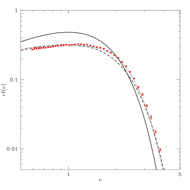
Figure 3: Collapsed mass fractions. The solid line represents the standard excursion set theory predictions. The dashed and dotted lines represent the improved fits of Sheth & Tormen Sheth and Tormen (1999) and Jenkins et al. Jenkins et al. (2001) respectively. The points represent numerical data from a suite of N-body simulations reluctantly provided by J. L. Tinker.

Analytic mass spectra are often compared to simulation data without reference to specific power spectra or cosmological models by comparing the fraction of mass in collapsed objects per logarithmic interval in $\nu$, $\nu f(\nu)\equiv\mathrm{d}F/\mathrm{d}\ln\nu$. For the standard excursion set theory,

$$f(\nu)=\sqrt{\frac{2}{\pi}}\exp\Bigg{(}-\frac{\nu^{2}}{2}\Bigg{)}.$$ (35)

In Fig. 3, I compare the Press-Schechter/Excursion set predictions for the fraction of mass in collapsed objects with the results of a suite of cosmological numerical simulations. While excursion set theory may explain the gross features of the mass spectrum of dark matter halos, it fails in its detail. The Press-Schechter/Excursion set relations predict too many low-mass halos and too few high-mass halos. Given the simplicity of the excursion set model described above, this is not surprising and the level of agreement provides encouragement that the excursion set model is a useful tool for understanding the gross features of halo abundance, formation, and clustering. In particular, these gross features are set by the statistics of the initial density fluctuations.

One detail not discussed so far is the assignment of mass to a particular filter radius $R$ or variance $S$. As I have already mentioned, the Press-Schechter relation follows directly by assuming a window function that is a tophat in Fourier space, but such a window does not have a well-defined volume to associate with it. The method of circumventing this that is implemented most often is to simply use the formulas derived from the sharp k-space filtering assumption, but assign mass according to a configuration space tophat filter so that $M=4\pi R^{3}/3\rho_{\mathrm{M}}$ (though this is not the method used by Bond et al. in Ref. Bond et al. (1991)).

In the context of excursion set theory, the k-space tophat window function serves only to simplify the solution for $\Pi(\delta,S)$ [Eq. (30)] and the first barrier up-crossing distribution [Eq. (32)]. In principle, other windows can be used but the mathematics become significantly more complicated. This is because the steps are no longer independent so it is necessary to compute the entire trajectory at once to account for the correlations between the steps. Ref. Bond et al. (1991) demonstrates the general procedure which amounts to generating a large number of solutions to a Langevin equation of random motion (e.g., , see Ref. Chandrasekhar (1943)) with a correlated stochastic force. Each solution yields a single trajectory of density at each value of the smoothing scale. The probability distributions can be computed from an ensemble of trajectories. This procedure is potentially complicated and time consuming, and it has the drawback that it does not yield a closed-form solution for the $\Pi(\delta,S)$ or first up-crossing distributions. For these reasons, other filters are rarely discussed; however, it is important to keep in mind that the lack of correlations between different steps is not a prediction of excursion set theory. Contrarily, it is a simplifying assumption used in the most common implementation of excursion set theory.

V Excursion Set Theory of the Spatial Bias of Dark Matter Halos

It has long been appreciated that within the context of cosmological structure formation theories, the clustering of dark matter halos differs from the overall clustering of matter Kaiser (1984); Efstathiou et al. (1988); Mo and White (1996); Sheth and Tormen (1999); Seljak and Warren (2004). The excursion set formalism provides a neat framework with which to understand the relative clustering of halos. The argument is much the same as the peak-background split approach developed in Refs. Kaiser (1984); Efstathiou et al. (1988); Cole and Kaiser (1989), and was expressed in the framework of the excursion set model by Mo & White Mo and White (1996) as I outline below.

Consider the solution to the excursion set problem in Eq. (30). This gives the probability distribution of $\delta$ given that on a smoothing scale $S_{0}$, the smoothed density fluctuation is $\delta_{0}$. Notice that the important quantity is the relative height of the density threshold $\delta_{\mathrm{c}}-\delta_{0}$ so that in regions with $\delta_{0}>0$ on large scales, trajectories are more likely to penetrate the barrier at $\delta_{\mathrm{c}}$ and conversely for $\delta_{0}<0$. This means that Eq. (31) and Eq. (32) allow for the calculation of the mass function in regions with specific large-scale density fluctuations.

The fraction of mass in collapsed halos of mass greater than $M$ in a region that has a smoothed density fluctuation $\delta_{0}$ on scale $S_{0}$ (corresponding to mass $M_{0}$ and volume $V_{0}$) is given by Eq. (31),

$$F(M|\delta_{0},S_{0})=\mathrm{erfc}\Bigg{(}\frac{\delta_{\mathrm{c}}-\delta_{0}}{2\Delta S}\Bigg{)}.$$ (36)

Notice that as the density of the region increases, $F$ increases because smaller upward excursions are needed to cross the threshold. When $\delta_{0}\to\delta_{\mathrm{c}}$, $F\to 1$ because the entire region will then be interpreted as a collapsed halo of mass $M_{0}$. The fraction of mass in halos with mass in the range $M$ to $M+\mathrm{d}M$ is

$$f(M|\delta_{0},S_{0})\Bigg{|}\frac{\mathrm{d}S}{\mathrm{d}M}\Bigg{|}\mathrm{d}M \equiv \frac{\mathrm{d}F(M|\delta_{0},S_{0})}{\mathrm{d}M}\mathrm{d}M$$ (37)

$$= \frac{1}{\sqrt{2\pi}}\frac{\delta_{\mathrm{c}}-\delta_{0}}{\Delta S^{3/2}}\Bigg{|}\frac{\mathrm{d}S}{\mathrm{d}M}\Bigg{|}\ \exp\Bigg{[}-\frac{(\delta_{\mathrm{c}}-\delta_{0})^{2}}{2\Delta S}\Bigg{]}\mathrm{d}M,$$

so that regions with smoothed density $\delta_{0}$ on scale $S_{0}$ contain, on average,

$$\mathcal{N}(M|\delta_{0},S_{0})\mathrm{d}M=\frac{M_{0}}{M}\ f(M|\delta_{0},S_{0})\Bigg{|}\frac{\mathrm{d}S}{\mathrm{d}M}\Bigg{|}\mathrm{d}M$$ (38)

halos in this mass range.

The quantity of interest is the relative over-abundance of halos in dense regions compared to the mean abundance of halos,

$$\delta_{\mathrm{halo}}^{\mathrm{L}}=\frac{\mathcal{N}(M|\delta_{0},S_{0})}{(\mathrm{d}n(M)/\mathrm{d}M)V_{0}}-1,$$ (39)

where $\mathrm{d}n(M)/\mathrm{d}M$ is the mean number density of halos in a mass range of width $\mathrm{d}M$ about $M$ from Eq. (34). The superscript $\mathrm{L}$ indicates that this is the overdensity in the initial Lagrangian space determined by the mass distribution at some very early time, ignoring the dynamical evolution of the overdense patch.

The relative overdensity of halos in large overdense and underdense patches is easy to compute. In sufficiently large regions, $S_{0}\ll S$, $\delta_{0}\ll\delta_{\mathrm{c}}$. Expanding Eq. (39) to first order in the variables $S_{0}/S$ and $\delta_{0}/\delta_{\mathrm{c}}$ gives a simple relation between halo abundance and dark matter density (see also Refs. Efstathiou et al. (1988); Cole and Kaiser (1989))

$$\delta_{\mathrm{halo}}^{\mathrm{L}}=\frac{\nu^{2}-1}{\delta_{\mathrm{c}}}\delta_{0},$$ (40)

where $\nu=\delta_{\mathrm{c}}/S^{1/2}=\delta_{\mathrm{c}}/\sigma(M)$ as before. The overdensity in the initial Lagrangian space is proportional to the dark matter overdensity and is a function of halo mass through $\nu$. The final ingredient needed to relate the abundance of halos to the matter density is a model for the dynamics that can map the initial Lagrangian volume to the final Eulerian space. Let $V$ and $\delta$ represent the Eulerian space variables corresponding to the Lagrangian space variables $V_{0}$ and $\delta_{0}$. The final halo abundance is

$$\delta_{\mathrm{halo}}=\frac{\mathcal{N}(M|\delta_{0},S_{0})}{(\mathrm{d}n(M)/\mathrm{d}M)V}-1.$$ (41)

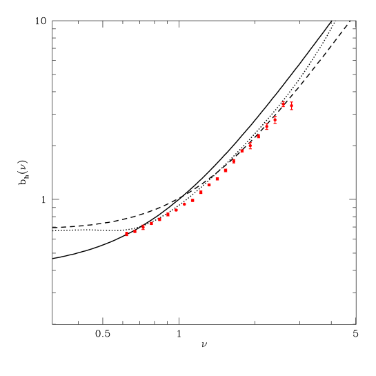
Figure 4: The large-scale bias of dark matter halos as a function of the scaled variable $\nu$. The solid line gives the prediction of the standard Press-Schechter or excursion set theory in Eq. (42). The dashed line is a modified form for the bias that follows from a modified form for the barrier criterion given by Sheth & Tormen in Ref. Sheth and Tormen (1999). The dotted line represents an empirical fit to N-body simulation results given by Seljak & Warren Seljak and Warren (2004). The points represent numerical data from a suite of N-body simulations kindly provided by J. L. Tinker.

Mo & White Mo and White (1996) give an extensive discussion of the mapping from Lagrangian to Eulerian coordinates and use a spherical collapse model to determine the appropriate mapping quantitatively. In the limit of a small overdensity $\delta_{0}\ll 1$, $V\simeq V_{0}(1+\delta)$, $\delta\simeq\delta_{0}$, and

$$\delta_{\mathrm{halo}} = \Bigg{(}1+\frac{\nu^{2}-1}{\delta_{\mathrm{c}}}\Bigg{)}\delta$$ (42)

$$\equiv b_{\mathrm{h}}\delta.$$ (43)

The halo overabundance is proportional to the matter overdensity and always has the same sense. This proportionality is commonly referred to has the halo bias $b_{\mathrm{h}}=(1+[\nu^{2}-1]/\delta_{\mathrm{c}})$. Interestingly, Eq. (42) gives a mass scale at which halos are not biased with respect to the dark matter. At a halo mass equal to the typical collapse mass, $M=M_{\star}$, $\nu=1$ or $\sigma(M)=\delta_{\mathrm{c}}$ so that the halo overdensity is the same as the total matter overdensity, $\delta_{\mathrm{halo}}=\delta$. Larger halos will have larger values of $\nu=\delta_{\mathrm{c}}/\sigma(M)$ because $\sigma(M)$ decreases with mass, so larger halos cluster considerably more strongly than the overall clustering of mass, while halos with $M<M_{\star}$ cluster more weakly than the overall mass distribution.

The large-scale halo bias relation of Eq. (42) is plotted as a function of scaled peak height $\nu$, in Fig. 4. In that figure, I also plot numerical results for the relative clustering bias of halos as well as improved fits for halo bias given by Sheth & Tormen Sheth and Tormen (1999) and Seljak & Warren Seljak and Warren (2004). The fit of Sheth & Tormen in Ref. Sheth and Tormen (1999) can be motivated by excursion set theory with a modified form for the shape of the barrier as a function of smoothing scale (e.g., Refs. Sheth et al. (2001); Sheth and Tormen (2002), and see § IX). These simple prescriptions for halo bias form one of the cornerstones of the analytic halo model that is often used to quantify the clustering of both dark matter and galaxies rapidly without resorting to a full numerical treatment Scherrer and Bertschinger (1991); Seljak (2000); Ma and Fry (2000); Peacock and Smith (2000); Berlind and Weinberg (2002). As with the mass function, the standard excursion set approach gives an understanding of the general features of the halo bias, but fails to reproduce the halo bias in detail.

VI An Excursion Set Model for Voids in the Galaxy Distribution

The excursion set model relates the initial density field on particular scales to specific structures in the evolved density field. To compute the properties of halos, one considers overdensities in the initial smoothed density field but it seems natural that this logic can be extended to underdense regions, and in particular, to voids in the density distribution. This is a particularly interesting application of the excursion set theory because of the relatively simple dynamics of underdense patches. Whereas overdense patches collapse, underdense patches expand more rapidly than the universal expansion rate. Contrary to the complicated behavior of overdensities, general underdense patches that are not initially spherically-symmetric, tophat underdensities evolve toward spherically-symmetric tophat underdensities  Icke (1984); Bertschinger (1985); van de Weygaert and Van Kampen (1993); Sheth and van de Weygaert (2004). This fact is encouraging. It suggests that a density threshold criterion based on a spherical, tophat model may be a more realistic model of void evolution than it is of the collapse of overdense patches.

Sheth & Van Weygaert Sheth and van de Weygaert (2004) made precisely this realization and applied the excursion set model to predict the abundance and sizes of voids in the universe. Most of the details of the excursion set model of voids can be found in their paper. The logic is quite similar to that of the previous two sections. First, it is necessary to assign a barrier height to designate a region that should be identified with a void, $\delta_{\mathrm{v}}<0$. (At this point, I reiterate that the overdensities that we consider are initial overdensities evaluated at some very early time, before any scales of interest have gone nonlinear, and extrapolated to $z=0$ using the linear theory of evolution so that overdensities are not constrained to $\delta\geq-1$.) The peculiar acceleration of a mass shell in a spherical underdense region is proportional to the integrated deficit in mass within the spherical region. A consequence of this is that inner shells accelerate outward faster than shells of mass on the outer edge of an underdense region. Mass shells start to accumulate in a narrow range of radii leading to a very high density ridge on the outer boundary of the underdense patch. Eventually, the inner shells overtake the outer shells at the moment of shell crossing. The relevant calculations are collected and reviewed in the appendices of Ref. Sheth and van de Weygaert (2004).

In the now defunct standard cold dark matter model with $\Omega_{\mathrm{M}}=1$, shell crossing for a spherical tophat overdensity occurs at a linearly-extrapolated overdensity of $\delta_{\mathrm{v}}=-2.81$. This is analogous to the case of spherical tophat overdensity collapse, where collapse to a point occurs when the linearly-extrapolated overdensity is $\delta_{\mathrm{c}}=1.69$. As with the spherical tophat overdensity, there is a weak dependence on cosmological parameters that I will ignore for the purposes of this discussion. Blumenthal et al. Blumenthal et al. (1992) argued that galaxy voids should be identified with regions that have just experienced shell crossing. Again, this is analogous to defining halos as regions that have just experienced complete collapse. In this case, the galaxies in the void walls would lie on the overdense ridges that form at shell crossing. The model of Sheth & Van Weygaert Sheth and van de Weygaert (2004) adopts this identification of voids with regions that just experience shell crossing and identify voids with the largest regions for which the smoothed density achieves the threshold $\delta_{\mathrm{v}}=-2.81$.

In contrast to the case of halos, voids present an additional challenge to computing the first crossing distribution. The additional difficulty is that an underdense region may be contained in a still larger overdense region which may collapse around the underdensity, engulfing and eliminating the void. Therefore, it is sensible that there be a second criterion that the smoothed density not exceed some overdensity threshold $\delta_{\mathrm{c}}^{\mathrm{v}}>0$, on some scale larger than the first crossing of $\delta_{\mathrm{v}}$. The appropriate height of the second barrier $\delta_{\mathrm{c}}^{\mathrm{v}}$ is not obvious. It is clear that $\delta_{\mathrm{c}}^{\mathrm{v}}\leq\delta_{\mathrm{c}}$ because a void cannot reside within a virialized halo. Thus, the least restrictive choice that can be made is $\delta_{\mathrm{c}}^{\mathrm{v}}=\delta_{\mathrm{c}}=1.69$. However, this does not account for the fact that some voids may be squeezed due to large-scale overdensities that have not yet collapsed and virialized and so it likely leads to an overestimate of the volume filling factor of voids in the universe. Sheth & Van Weygaert Sheth and van de Weygaert (2004) also explore $\delta_{\mathrm{c}}^{\mathrm{v}}=1.06$ as this linearly-extrapolated overdensity corresponds to the moment of turnaround, or the transition from expansion to contraction, for a spherical overdensity. The drawback of this choice is that it completely erases voids in regions that are only just turning around so that this choice likely leads to an underestimate of the filling factor of voids in the universe. This discussion suggests that the appropriate value of the “void-squashing” overdensity should be in the range $1.06<\delta_{\mathrm{c}}^{\mathrm{v}}<1.69$.

The first step in modeling the void population with the excursion set theory should now be clear. It is necessary to solve for the first crossing distribution of the barrier $\delta_{\mathrm{v}}$ subject to the additional restriction that the barrier at $\delta_{\mathrm{c}}^{\mathrm{v}}$ is not achieved at some larger scale either. As in § IV, it is convenient to solve for the probability distribution of trajectories that do not impact either barrier $\Pi(\delta,S)$, and to derive the first-crossing distribution from $\Pi(\delta,S)$. As before, the distribution of $\delta$ at any value of $S$ obeys

$$\frac{\partial\Pi}{\partial S}=\frac{1}{2}\frac{\partial^{2}\Pi}{\partial\delta^{2}}.$$ (44)

In the case of voids, trajectories are removed from consideration when they impinge upon either of the two barriers at $\delta_{\mathrm{c}}^{\mathrm{v}}$ or $\delta_{\mathrm{v}}$ so that the boundary conditions are $\Pi(\delta_{\mathrm{v}},S)=\Pi(\delta_{\mathrm{c}}^{\mathrm{v}},S)=0$.

This system of equations is the one-dimensional heat equation describing heat flow in a long, thin bar of finite length held at fixed temperature at both ends. As such, it has a solution that is likely to be familiar. To begin with, unlike the case of the single-barrier problem in § IV, the solution to this boundary value problem can only be a superposition of a discrete set of sinusoidal modes, namely those modes that individually obey the homogeneous boundary conditions.

As before, it is convenient to define a new variable $\gamma\equiv\delta-\delta_{\mathrm{v}}$. In that case, Eq. (44) still holds with $\delta$ replaced by $\gamma$ and the boundary conditions are $\Pi(\gamma=0,S)=\Pi(\gamma=\gamma_{\mathrm{c,v}}=\delta_{\mathrm{c}}^{\mathrm{v}}-dv,S)=0$. As before, trajectories start at $\delta=0$ at $S=0$ so that the initial condition is $\Pi(\gamma,S=0)=\delta_{\mathrm{D}}(\gamma+\delta_{\mathrm{v}})$. The solution follows straightforwardly using separation of variables. Assuming that $\Pi(\gamma,S)=G(\gamma)P(S)$, the functions $G(\gamma)$ and $P(S)$ obey

$$\frac{1}{P}\frac{\mathrm{d}P}{\mathrm{d}S}=\frac{1}{2G}\frac{\mathrm{d}^{2}G}{\mathrm{d}\gamma^{2}}=-k^{2},$$ (45)

where $k$ is some constant. Therefore $P(S)\propto\exp(-k^{2}\ S)$. The boundary conditions on $G(\gamma)$ can only be satisfied if $k>0$. Thus the solution is a superposition of sines and cosines. It is easy to show that the boundary conditions require that

$$G(\gamma)=\sum_{n=1}^{\infty}\ c_{n}\ \sin\Bigg{(}\frac{n\pi}{\gamma_{\mathrm{c,v}}}\gamma\Bigg{)}.$$ (46)

The initial condition can be used to determine the $c_{n}$ by using the orthogonality relation for sinusoids, $\int_{0}^{\pi}\ \sin(ny)\ \sin(my)\mathrm{d}y=(\pi/2)\delta_{nm}$, where $\delta_{nm}$ is a Kronecker delta. The result is that $c_{n}=2\sin(n\pi|\delta_{\mathrm{v}}|/\gamma_{\mathrm{c,v}})/\pi$. Consequently, the solution to the boundary value problem is

$$\Pi(\delta,S) = \frac{1}{\delta_{\mathrm{c}}^{\mathrm{v}}-\delta_{\mathrm{v}}}\sum_{n=1}^{\infty}\ \Bigg{[}\cos\Bigg{(}\frac{n\pi}{\delta_{\mathrm{c}}^{\mathrm{v}}-\delta_{\mathrm{v}}}\delta\Bigg{)}\ -\ \cos\Bigg{(}\frac{n\pi}{\delta_{\mathrm{c}}^{\mathrm{v}}-\delta_{\mathrm{v}}}[2\delta_{\mathrm{v}}-\delta]\Bigg{)}\Bigg{]}\$$ (47)

$$\ \ \times\exp\Bigg{(}-\frac{n^{2}\pi^{2}}{2(\delta_{\mathrm{c}}^{\mathrm{v}}-\delta_{\mathrm{v}})}S\Bigg{)}.$$

In analogy with Eq. (31) and Eq. (32), trajectories are removed from the region between the two boundaries at a “rate” of

$$f_{\mathrm{v}}(S)\mathrm{d}S=-\frac{1}{2}\frac{\partial\Pi}{\partial\delta}\Bigg{|}_{\delta_{\mathrm{v}}}^{\delta_{\mathrm{c}}^{\mathrm{v}}}\ \mathrm{d}S.$$ (48)

The lower limit of this divergence of trajectories indicates the trajectories that penetrate the lower boundary at $\delta=\delta_{\mathrm{v}}$. These are the void regions that we aim to model, so the first crossing distribution is

$$f_{\mathrm{v}}(S)\mathrm{d}S = \frac{1}{2}\frac{\partial\Pi}{\partial\delta}\Bigg{|}_{\delta_{\mathrm{v}}}$$ (49)

$$= \sum_{n=1}^{\infty}\ \frac{n\pi\mathcal{D}^{2}}{\delta_{\mathrm{v}}^{2}}\ \sin(n\pi\mathcal{D})\ \exp\Bigg{(}-\frac{n^{2}\pi^{2}\mathcal{D}^{2}}{2}\frac{S}{\delta_{\mathrm{v}}^{2}}\Bigg{)}\mathrm{d}S,$$

where $\mathcal{D}\equiv|\delta_{\mathrm{v}}|/(\delta_{\mathrm{c}}^{\mathrm{v}}+|\delta_{\mathrm{v}}|)$ is the void-in-cloud parameter, following the nomenclature of Ref. Sheth and van de Weygaert (2004). The parameter $\mathcal{D}$ quantifies the relative importance of eliminating voids that lie within some larger overdense region in which the smoothed density contrast exceeds $\delta_{\mathrm{c}}^{\mathrm{v}}$.

Figure 5: Left: The mass distribution of voids predicted by the excursion set model of Sheth & Van Weygaert Sheth and van de Weygaert (2004). The mass distribution is given in scaled units. The horizontal axis is the absolute value of the void threshold in units of the $\sigma(M)$ for a particular mass scale $\nu_{\mathrm{v}}=|\delta_{\mathrm{v}}|/S^{1/2}$. The vertical axis is the fraction of trajectories that first cross the threshold in a logarithmic interval of $\nu_{\mathrm{v}}$. Physically, this is the fraction of mass in voids that have a mass corresponding to a logarithmic interval in $\nu_{\mathrm{v}}$. The three lines show three choices of the overdensity threshold $\delta_{\mathrm{c}}^{\mathrm{v}}$. Right: The physical size distribution of voids. The three lines represent the number densities of voids of radius $R$ for the same three choices of $\delta_{\mathrm{c}}^{\mathrm{v}}$ as in the left panel.

From the first-crossing distribution of Eq. (49), it is straightforward to compute the “mass function” of voids, meaning the number of voids containing a specific amount of mass. As before, it is most convenient to represent this distribution in terms of a scaled variable $\nu_{\mathrm{v}}\equiv|\delta_{\mathrm{v}}|/S^{1/2}$, so that the physical size distribution is determined by the size of the smoothing scale at a particular value of the variance $S$ and the parameter $\mathcal{D}$. Then $\nu_{\mathrm{v}}f_{\mathrm{v}}(\nu_{\mathrm{v}})$ defined as the fraction of mass in voids per logarithmic interval $\mathrm{d}\ln\nu_{\mathrm{v}}$ then follows by changing variables in Eq. (49) from $S$ to $\nu_{\mathrm{v}}$ as in § IV. Explicitly,

$$\nu_{\mathrm{v}}f_{\mathrm{v}}(\nu_{\mathrm{v}})=\sum_{n=1}^{\infty}\ \frac{2n\pi\mathcal{D}^{2}}{\nu^{2}}\ \sin(n\pi\mathcal{D})\ \exp\Bigg{(}-\frac{n^{2}\pi^{2}\mathcal{D}^{2}}{2\nu^{2}}\Bigg{)}.$$ (50)

This void mass spectrum is shown in the left panel of Fig. 5 for the choices of $\delta_{\mathrm{v}}=-2.81$ and $\delta_{\mathrm{c}}^{\mathrm{v}}=1.06$ advocated by Sheth & Van Weygaert Sheth and van de Weygaert (2004). Two additional mass spectra derived from different values of $\delta_{\mathrm{c}}^{\mathrm{v}}$ are shown in Fig. 5 to illustrate the importance of the void-in-cloud parameter. The choice $\delta_{\mathrm{c}}^{\mathrm{v}}\to\infty$ corresponds to ignoring completely the possibility for a larger-scale overdensity to overwhelm a smaller void within it. Decreasing $\delta_{\mathrm{c}}^{\mathrm{v}}$ makes the probability for a larger overdensity to overwhelm a void within it higher and decreases the number of voids of all sizes. Two things are worthy of note. First, the number of large voids (high $\nu_{\mathrm{v}}$) is independent of $\delta_{\mathrm{c}}^{\mathrm{v}}$. This is because it is very unlikely for a trajectory to cross both the $\delta_{\mathrm{c}}^{\mathrm{v}}$ and the $\delta_{\mathrm{v}}$ thresholds at small values of $S$. Second, regardless of the choice of $\delta_{\mathrm{c}}^{\mathrm{v}}$, the fraction of mass in voids is peaked around voids with $\nu_{\mathrm{v}}\approx 1-1.5$. This places the typical void mass in the broad range $M_{\mathrm{void}}\sim 10^{11}-10^{13}\ h^{-1}\mathrm{M}_{\odot}$. Of course, as with the mass function, the number of voids of a particular size will be shifted toward smaller objects because a fixed fraction of mass can be partitioned into more small voids and fewer large voids.

The void size spectrum in Eq. (50) gives the fraction of mass, or of volume in the initial Lagrangian space, in voids of a particular size. The size variable is the scaled variable $\nu_{\mathrm{v}}$. To convert this to a physical size spectrum where the sizes of objects are measured in units of length or volume requires relating the initial Lagrangian volume to an Eulerian volume. The simplest conversion follows from the fact that in the spherical tophat model, the tophat radius expands by a factor or $\sim 1.72$ by the time shell crossing occurs. Finally, one also needs to assume a power spectrum to relate particular values of $\nu_{\mathrm{v}}$ with volume in the initial Lagrangian coordinate system. As before, I will assume the spectrum in Fig. 1. The logic is then the same as that of the mass function. The number density of voids as a function of physical void radius is shown in the right panel of Fig. 5 and reflects the basic features of the voids model. The number density of voids is independent of $\delta_{\mathrm{c}}^{\mathrm{v}}$ for large voids, and the number of small voids is suppressed because small, underdense regions are likely to be contained within larger overdense regions.

So far, I have ignored the primary shortfall of the void model. The weakness of the approach of Ref. Sheth and van de Weygaert (2004) is that it defines a void as a region that is underdense with respect to total mass whereas observationally voids are identified as underdensities in the galaxy distribution, as noted in Ref. Sheth and van de Weygaert (2004). Furlanetto & Piran Furlanetto and Piran (2005) have extended the Sheth & Van Weygaert model to identify voids as regions that are underdense in the galaxy distribution. To do this, these authors added to the excursion set theory a method for assigning galaxies to halos and thereby established a mapping between the galaxy number density in a region and a linearly-extrapolated overdensity. Methods for assigning galaxies to halos are beyond the scope of this article so I will not discuss the model of Ref. Furlanetto and Piran (2005) any further except to say that it is a more practical approach to voids because it phrases predictions in terms of the observed galaxy overdensity.

VII Halo Formation in the Excursion Set Theory

Excursion set theory is also a powerful formalism with which to study the formation history of halos. It is most natural to picture evolution occuring through the linear growth of the density field. In that way, the smoothed overdensity scales with time according to the linear growth factor $D(a)$. Writing the smoothed density field as a function of both the smoothing scale $S$ and the cosmological expansion factor $a$, this evolution is $\delta(S,a)=D(a)\delta(S,a=1)$. As a matter of convention, $D(a)$ is normalized so that $D(a=1)=1$. In the framework of excursion sets, predictions depend upon the density field in the ratio $\nu=\delta_{\mathrm{c}}/\sigma(M)$ and it is often easier to envision the density field as fixed at $\delta(S)\equiv\delta(S,a=1)$ and to consider the height of the critical density threshold as a function of time. In that way, collapse at a scale factor $a^{\prime}\neq 1$ corresponds to the $a=1$ density fluctuation penetrating a barrier of height $\delta_{\mathrm{c}}(a^{\prime})=\delta_{\mathrm{c}}/D(a^{\prime})$.

In their pioneering paper, Bond et al. Bond et al. (1991) briefly discussed the utility of the excursion set approach for understanding the formation histories of halos. Subsequently, Lacey & Cole Lacey and Cole (1993) studied this problem in great detail in a rather elegant paper and I largely follow their treatment in what follows. I will adopt the simplifying notation of Ref. Lacey and Cole (1993) and refer to the barrier height for collapse at a specific time as

$$\omega(a)\equiv\delta_{\mathrm{c}}/D(a).$$ (51)

The variable $\omega$ indicates the time of the collapse through only the linear growth function $D(a)$. In the “old standard” CDM model with $\Omega_{\mathrm{M}}=1$, the growth function is simply $D(a)=a$ and the conversion between $\omega$ and $a$ is trivial. However, in the currently-favored $\Lambda$CDM model, the growth function is given by an incomplete beta function integral Bildhauer et al. (1992) and the conversion is more complicated.

Many of the insights into halo formation can be gleaned by considering the two-barrier problem, just as with halo bias and void regions in the previous two sections. Again following the work of Lacey & Cole Lacey and Cole (1993), I also adopt a simplifying notation for the conditional probabilities of barrier crossings. I illustrate this notation by re-writing the two-barrier probability distribution already given in Eq. (32) and Eq. (37) as

$$f(S_{2},\omega_{2}|S_{1},\omega_{1})\mathrm{d}S_{2}=\frac{1}{\sqrt{2\pi}}\frac{\Delta\omega}{\Delta S^{3/2}}\ \exp\Bigg{[}-\frac{(\Delta\omega)^{2}}{2\Delta S}\Bigg{]}\mathrm{d}S_{2},$$ (52)

where $\Delta\omega\equiv\omega_{2}-\omega_{1}$ is the difference between the two barrier heights (assumed to be arbitrary with $\omega_{2}>\omega_{1}$), $\Delta S\equiv S_{2}-S_{1}$. As always, some mass $M_{1}$ and $M_{2}$ are associated with the variances $S_{1}$ and $S_{2}$ respectively. The quantity $f(S_{2},\omega_{2}|S_{1},\omega_{1})\mathrm{d}S_{2}$ is the conditional probability that a trajectory pierces the barrier $\omega_{2}$ in an interval of width $\mathrm{d}S_{2}$ about $S_{2}$ on the condition that the trajectory first pierces $\omega_{1}$ at $S_{1}$. As a further shorthand, I take $f(S_{2},\omega_{2})\mathrm{d}S_{2}$ to denote the probability starting from a very large smoothing scale $S_{1}=0$, and $\omega_{1}=0$.

In this section and those that follow, the interpretation of Eq. (52) is different from that in § IV and § V. In those sections, the initial condition for the random walk was fixed by the large scale environment on some larger filtering scale $S_{1}\ll S_{2}$. Here, the two barriers represent the critical density for collapse at two different times so the change in barrier height $\Delta\omega$ represents a shift in time.

VII.1 The Conditional Mass Function

Figure 6: The conditional mass function. All panels refer to the conditional mass functions of halos fixed at $z=0$ looking back toward higher redshifts as labeled in each panel. Four halo masses of interest are shown.

The most immediate quantity of interest is the conditional mass function. Given a halo of mass $M_{1}$ at time $t_{1}$, one can compute the average manner in which this mass was partitioned among smaller halos at some earlier time $t_{2}<t_{1}$ ($\omega_{2}>\omega_{1}$). The conditional mass function is simply the average number of halos of mass $M_{2}$ at time $t_{2}$ that are incorporated into a mass $M_{1}$ object at time $t_{1}$. This is precisely the two-barrier problem. A halo of mass $M_{1}$ has its mass partitioned, on average, among a spectrum of halos at time $w_{2}$ given almost directly from Eq. (52) (e.g., see Refs. Lacey and Cole (1993); Somerville and Kolatt (1999)),

$$\frac{\mathrm{d}n(M_{2}|M_{1})}{\mathrm{d}M_{2}}=\frac{M_{1}}{M_{2}}\ f(S_{2},\omega_{2}|S_{1},\omega_{1})\ \Bigg{|}\frac{\mathrm{d}S_{2}}{\mathrm{d}M_{2}}\Bigg{|}\mathrm{d}M_{2}.$$ (53)

The function $f(S_{2},\omega_{2}|S_{1},\omega_{1})$ gives the probability of the second barrier crossing at a particular value of $S_{2}$, while the factor $M_{1}/M_{2}$ converts this from a probability per unit mass of halo $M_{1}$ into the number of halos of mass $M_{2}$.

Figure 6 shows conditional mass functions for standard CDM power spectra normalized such that $M_{\star}=10^{13}\ h^{-1}\mathrm{M}_{\odot}$ ($\sigma_{8}\simeq 0.93$) for four halo masses at four different lookback redshifts, $z=1/4$, $z=1/2$, $z=1$, and $z=3$ (all panels have final redshift at $z=0$). The evolution toward increased fragmentation as the second epoch moves to higher redshifts is evident. Notice that more massive halos fragment into small sub-units more quickly. Also, notice that each conditional mass function goes toward an approximate power law as $M_{2}/M_{1}\ll 1$. This can be understood directly from Eq. (6). Assume that the power spectrum is an approximate power law $S(M)\simeq\delta_{\mathrm{c}}^{2}(M/M_{\star})^{-\beta}$ in the mass range of interest. In the limit of a large mass difference, $\Delta\omega/\Delta S\ll 1$ and $M_{2}/M_{1}\ll 1$ and $\mathrm{d}n/\mathrm{d}M_{2}\propto M_{2}^{-(4-3\beta)/2}$. Near $M_{\star}$, CDM-like power spectra vary slowly, with an effective power-law index near $\beta\approx 0.35$ giving $\mathrm{d}n/\mathrm{d}M_{2}\propto M_{2}^{-3/2}$, which is approximately the power law shown in Figure 6.

VII.2 Halo Accretion Rates

The excursion set theory also provides a framework for computing mass accretion rates as well. The two-barrier problem of § VII.1 can be manipulated to yield an average mass accretion rate. Consider the probability of transitioning forward in time, from $M_{2}$ at barrier $\omega_{2}$ to $M_{1}$ at $\omega_{1}$. Bayes’ rule for combining probabilities gives the forward probability as Lacey and Cole (1993)

$$f(S_{1},\omega_{1}|S_{2},\omega_{2})\mathrm{d}S_{1} = \frac{f(S_{2},\omega_{2}|S_{1},\omega_{1})f(S_{1},\omega_{1})}{f(S_{2},\omega_{2})}\mathrm{d}S_{1}$$ (54)

$$= \frac{1}{\sqrt{2\pi}}\frac{\omega_{1}(\omega_{2}-\omega_{1})}{\omega_{2}}\Bigg{[}\frac{S_{2}}{S_{1}(S_{2}-S_{1})}\Bigg{]}^{3/2}$$ (56)

$$\times\exp\Bigg{(}-\frac{(\omega_{1}S_{2}-\omega_{2}S_{1})}{2S_{1}S_{2}(S_{2}-S_{1})}\Bigg{)}\ \mathrm{d}S_{1}.$$

In language familiar to cosmology, $f(S_{1},\omega_{1}|S_{2},\omega_{2})$ is the posterior probability, $f(S_{1},\omega_{1})$ is the prior, and $f(S_{2},\omega_{2}|S_{1},\omega_{1})$ is the likelihood.

Figure 7: Halo accretion rates per logarithmic interval of mass change. This is based on a very similar plot in Ref. Lacey and Cole (1993). The plots show the accretion rates per unit mass change for halos of five different masses (shown in the left panel) at $z=0$. The left panel shows the probability for a change $\Delta M$ as a function of $\Delta M$ [Eq. (58)], while the right panel shows the fractional mass accretion rate given by $(\Delta M/M_{2})\times\mathrm{d}^{2}R/\mathrm{d}\ln\Delta M\mathrm{d}\ln a$.

The instantaneous probability per unit shift in barrier height follows by taking $\Delta\omega=(\omega_{2}-\omega_{1})\to 0$ in Eq. (54), giving

$$\frac{\mathrm{d}^{2}R}{\mathrm{d}\omega\ \mathrm{d}S_{1}}=\frac{1}{\sqrt{2\pi}}\Bigg{[}\frac{S_{2}}{S_{1}(S_{2}-S_{1})}\Bigg{]}^{3/2}\exp\Bigg{[}-\frac{\omega^{2}(S_{2}-S_{1})}{2S_{2}S_{1}}\Bigg{]},$$ (57)

from which the probability per unit change in mass $\Delta M=M_{1}-M_{2}$, per unit time (or $\mathrm{d}\ln a=H(a)\mathrm{d}t$) is

$$\frac{\mathrm{d}^{2}R}{\mathrm{d}\ln\Delta M\mathrm{d}\ln a} = \sqrt{\frac{2}{\pi}}\frac{\Delta M}{M_{1}}\frac{\omega/\sigma(M_{1})}{(1-S_{1}/S_{2})^{3/2}}$$ (58)

$$\times\exp\Bigg{[}-\frac{\omega^{2}(S_{2}-S_{1})}{2S_{1}S_{2}}\Bigg{]}\Bigg{|}\frac{\mathrm{d}\ln\omega}{\mathrm{d}\ln a}\Bigg{|}\Bigg{|}\frac{\mathrm{d}\ln\sigma}{\mathrm{d}\ln M_{1}}\Bigg{|}.$$

The average rate of mass accretion per unit change in mass can be obtained by multiplying Eq. (58) by $\Delta M$, while the average total mass accretion rate follows from multiplying Eq. (58) by $\Delta M$ and integrating over $\ln\Delta M$.

Figure 8: Total halo mass accretion rates in units of halo mass and as a function of halo mass at four different redshifts.

The excursion set accretion rates of halos in the standard $\Lambda$CDM cosmology are summarized in Fig. 7 and Fig. 8. The left panel Fig. 7 shows the probability for a particular fractional mass change as a function of the fractional mass change. The rate of accretion by small mass increments diverges. However, the average rate of mass increase (in the right panel of Fig. 7) converges and is dominated by the less frequent, high-mass mergers. Notice in particular that low-mass halos increase their masses very quickly via mergers with halos larger then themselves while halos with $M\lower 2.58334pt\vbox{\hbox{$\buildrel\textstyle>\over{\sim}\ $}}M_{\star}$ experience only infrequent mergers with halos larger than themselves.

The total mass accretion rate given by integrating Eq. (58) over $\ln\Delta M$ is shown in Fig. 8 for various redshifts as a function of halo masses. Fig. 8 shows explicitly that low-mass halos should be expected increase there mass many times over in a single Hubble time. The standard interpretation of the collection of results shown in Fig. 7 and Fig. 8 is that low-mass halos ($M<M_{\star}$) should be expected to increase their masses by mergers with halos larger than themselves, while high-mass halos ($M>M_{\star}$) typically absorb smaller halos and increase their masses relatively slowly.

VII.3 Halo Formation Times

It is often useful to have a sense of a time by which a halo acquired most of its mass. For example, one may be modeling galaxies and may try to estimate stellar evolution histories within a particular halo. Several definitions of halo formation time exist. An intuitive definition is the time that a halo first acquires half of its final mass because once a progenitor of a halo has achieved this threshold it can uniquely be identified as the main progenitor of the final object. Consider the formation time given by this definition $\omega_{\mathrm{F}}$ or, in terms of expansion factor, $a_{\mathrm{F}}$.

It is not trivial to predict halo formation times from excursion set theory by considering the two-barrier problem as before. The reason for this difficulty is simple to understand. Consider the formation of a halo of mass $M_{1}$ at time $\omega_{1}$. The probability of crossing a higher threshold $\omega_{2}$ (corresponding to earlier time) at some value of the variance greater than $S_{2}=S(M_{2}=M_{1}/2)>S_{1}$ gives only the probability per unit mass that the halo has some progenitor with mass $M_{2}\leq M_{1}/2$ at time $\omega_{2}$. It does not guarantee that this is the mass of the most massive of all of the subunits that merged to form the halo of mass $M_{1}$ at $\omega_{1}$. Lacey & Cole Lacey and Cole (1993) circumvent this difficulty by giving an approximate counting argument for the formation time. I reproduce the argument of Ref. Lacey and Cole (1993) in what follows.

First, the results of § VII.2 give the number of halos of mass $M_{2}$ at time $t_{2}$ that are incorporated into halos of mass $M_{1}$ at $t_{1}>t_{2}$ as

$$\frac{\mathrm{d}^{2}n}{\mathrm{d}M_{2}\mathrm{d}S_{1}}=\frac{\mathrm{d}n(M_{2})}{\mathrm{d}M_{2}}\ f(S_{1},\omega_{1}|S_{2},\omega_{2}).$$ (59)

So long as $M_{2}>M_{1}/2$, each trajectory must connect two unique halos because there cannot be two paths each of which contain more than half of the final halo mass. However, it is possible that a halo of mass $M_{1}$ at $t_{1}$ has no progenitor of mass greater than $M_{1}/2$ at time $t_{2}$. The counting argument accounts for this. The probability that a halo of mass $M_{1}$ at $t_{1}$ has a progenitor in the mass range $M_{1}\geq M_{2}>M_{1}/2$ at time $t_{2}$ is then given by the ratio of halos that evolve to a halo of mass $M_{1}$ relative to the total number of halos of mass $M_{1}$,

$$\frac{\mathrm{d}P}{\mathrm{d}M_{2}}=\frac{[\mathrm{d}n(M_{2})/\mathrm{d}M_{2}]f(S_{1},\omega_{1}|S_{2},\omega_{2})}{[\mathrm{d}n(M_{1})/\mathrm{d}M_{1}]||\mathrm{d}S_{1}/\mathrm{d}M_{1}|^{-1}}.$$ (60)

Using Bayes’ rule again and the definitions of the mass functions in terms of the first-crossing distributions gives

$$\frac{\mathrm{d}P}{\mathrm{d}M_{2}}=\Bigg{(}\frac{M_{1}}{M_{2}}\Bigg{)}\ f(S_{2},\omega_{2}|S_{1},\omega_{1})\Bigg{|}\frac{\mathrm{d}S_{2}}{\mathrm{d}M_{2}}\Bigg{|}.$$ (61)

The cumulative probability of a formation time prior to time $t_{2}$ is then the integral

$$P(t_{\mathrm{F}}<t_{2})=P(\omega_{\mathrm{F}}>\omega_{2})=\int_{S_{1}}^{S_{2}=S(M_{1}/2)}\ \Bigg{(}\frac{M_{1}}{M_{2}}\Bigg{)}f(S_{2}^{\prime},\omega_{2}|S_{1},\omega_{1})\mathrm{d}S_{2}^{\prime},$$ (62)

and the differential probability can be obtained by differentiating Eq. (62) with respect to either $\omega_{\mathrm{F}}$ or $t_{\mathrm{F}}$.

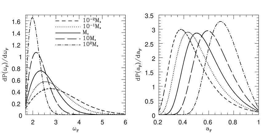
Figure 9: The probability distributions for formation times in the standard $\Lambda$CDM cosmology with a scale-invariant primordial power spectrum normalized to $\sigma_{8}=0.93$, so that $M_{\star}=10^{13}\ h^{-1}\mathrm{M}_{\odot}$. The left panel shows the distribution as a function of threshold height $\mathrm{d}P(\omega_{\mathrm{F}})/\mathrm{d}\omega_{\mathrm{F}}$ while the right panel shows the probability distribution of formation scale factors $\mathrm{d}P(a_{\mathrm{F}})/\mathrm{d}a_{\mathrm{F}}$.

Formation time distributions computed from Eq. (62) are shown in Fig. 9 for a variety of halo masses at $z=0$ ($a=1$, $\omega_{\mathrm{F}}=\delta_{\mathrm{c}}\simeq 1.69$). The most obvious feature of formation times is that small halos form early and large halos form relatively late in accordance with our general expectation in hierarchical models of structure formation. Note also that in the simplest implementation of the excursion set formalism, in particular making use of k-space tophat filtering of the density field, the conditional probability $f(S_{2},\omega_{2}|S_{1},\omega_{1})$ is a function only of the differences $S_{2}-S_{1}$ and $\omega_{2}-\omega_{1}$. In this case, this means that the formation times in particular and, more generally, the entire formation histories of halos are independent of the larger-scale environments that halos reside in. In the next section, I discuss halo formation times in the context of halo merger trees.

VIII Halo Merger Trees

The probability of first up-crossing at a second barrier given a particular starting point is given by the solution to the two-barrier problem in Eq. (52). This relation has been repeated several times throughout these notes in several forms because it is the fundamental relation on which most physical results are based. In the preceding sections, I have applied this formula to derive relations about various aspects of halo fragmentation and formation over time. So far, these quantities have been averages (as in § VII.1 and § VII.2) or probability distributions (as in § VII.3). However, as Ref. Lacey and Cole (1993) describes, the interpretation of Eq. (52) as a probability for a transition from one barrier to another means that one should be able to draw specific fragmentation probabilities from this distribution repeatedly for a number of time intervals $\Delta\omega_{i}$, and thereby reconstruct individual trajectories of halo mass versus cosmic expansion factor. This enables one to follow the fragmentation of halos on an object-by-object basis. This is the logic behind the algorithm for the generation of Monte Carlo merger trees described by (see also earlier methods in Refs. Cole and Kaiser (1988); Cole (1991); Kauffmann et al. (1993)).

The trajectories $\delta(S)$ have structure on arbitrarily small scales corresponding to mergers with very small halos. This is a restatement of the divergence of the mean number of transitions with small mass changes shown in the left panel of Fig. 7. Consequently, it is necessary to examine trajectories with a particular resolution in order to “smooth over” the mergers with numerous tiny halos. In practice, each application to the prediction of a specific physical quantity has a minimum mass scale of interest $M_{\mathrm{min}}$, so it is natural to set the resolution with which trajectories are computed according to this minimum scale. Consider Eq. (52) in the limit $\Delta\omega/\sqrt{\Delta S}\ll 1$. This gives a transition probability $f=\Delta\omega/(\sqrt{2\pi}\Delta S^{3/2})$, that is directly proportional to the time interval $\Delta\omega$. Lacey & Cole Lacey and Cole (1993) interpreted this as indicative of a probability that is due to a single, improbable merger event. For this reason, Lacey & Cole refer to the limit $\Delta\omega/\sqrt{\Delta S}\ll 1$ as the “binary regime.” This can be used to motivate a particular choice of step-size $\Delta\omega$ that sets the resolution of the trajectory.

First, consider making the change of variable to $u\equiv\Delta\omega/\sqrt{\Delta S}$ in Eq. (52). This converts the probability distribution to a Gaussian in the variable $u$ with a mean of zero and a unit variance. Of course, the probability distribution is one-sided in that it is subject to the constraint $u\geq 0$. To resolve individual, binary mergers of a parent halo of mass $M$ with a merging halo at the threshold $M_{\mathrm{min}}$ the step-size should obey

$$\Delta\omega\lower 2.58334pt\vbox{\hbox{$\buildrel\textstyle<\over{\sim}\ $}}\sqrt{\Bigg{|}\frac{\mathrm{d}S(M)}{\mathrm{d}M}\Bigg{|}M_{\mathrm{min}}},$$ (63)

so that these mergers are in the binary regime. Authors often parameterize this guideline and set $\Delta\omega=f_{\mathrm{step}}\sqrt{|\mathrm{d}S/\mathrm{d}M|M_{\mathrm{min}}}$. The guideline in Eq. (63) makes a transition with $\Delta M\geq M_{\mathrm{min}}$ a rare event. The motivation behind this choice is that it is very unlikely that the transition could be due to two rare events, so that most mergers with objects of mass $>M_{\mathrm{min}}$ are resolved as binary encounters. In particular, the probability for a transition with $\Delta M\geq M_{\mathrm{min}}$ is

$$P(>\Delta M) = \frac{2}{\sqrt{\pi}}\int_{0}^{f_{\mathrm{step}}/\sqrt{2}}\exp(-y^{2})\mathrm{d}y$$

$$= \mathrm{erf}(f_{\mathrm{step}}/\sqrt{\pi})$$

$$\approx \sqrt{\frac{2}{\pi}}f_{\mathrm{step}},$$

where the last step assumes $f_{\mathrm{step}}\ll 1$. The choice of $f_{\mathrm{step}}$ is motivated by the need to resolve all mergers of objects of mass $M_{\mathrm{min}}$, driving $f_{\mathrm{step}}$ toward small values, and the desire to spend as little effort as possible computing the probabilities for transitions with $\Delta M<M_{\mathrm{min}}$, driving $f_{\mathrm{step}}$ toward large values. As I discuss below Ref. Somerville and Kolatt (1999) advocates $f_{\mathrm{step}}\lower 2.58334pt\vbox{\hbox{$\buildrel\textstyle<\over{\sim}\ $}}0.3$ in order to guarantee accuracy down to $M_{\mathrm{min}}$. Typical values are $f_{\mathrm{step}}\lower 2.58334pt\vbox{\hbox{$\buildrel\textstyle<\over{\sim}\ $}}0.1$.

With these preliminaries out of the way, the Lacey & Cole Lacey and Cole (1993) algorithm for generating merger histories is as follows. First, determine the appropriate timestep using Eq. (63). Second, select a transition $\Delta S$ from the probability distribution of Eq. (52) and invert the $S(M)$ relation to obtain both the change in mass $\Delta M$ and the new main progenitor mass $M^{\prime}=M-\Delta M$. One then repeats this procedure at the new values of $\omega$ and $S(M^{\prime})$ in order to determine the next fragmentation of the main progenitor. This process continues until the remaining mass is less than $M_{\mathrm{min}}$.

The trajectory for the main progenitor, defined as the most massive progenitor at each timestep according to this algorithm, may form the trunk of a “merger tree.” All of the merging halos of mass $\Delta M$ have prior fragmentation histories of their own. For each mass $\Delta M$ above the threshold $M_{\mathrm{min}}$, one can generate an independent history for the infalling “branch” on the tree using the same algorithm.

The process of constructing a mass accretion history or merger tree in this way must be repeated numerous times in order to sample the variety of ways in which a halo of a fixed mass at a fixed time might build up its mass. This is a Monte Carlo method for exploring the various mass accretion histories. It is conventional to refer to each individual tree generated in this way as a particular realization in an ensemble of merger histories.

The algorithm for generating Monte Carlo merger trees described above is convenient because of its simplicity. Unfortunately, while this algorithm conserves mass by construction, it overpredicts the number of progenitor halos with masses $M>M_{\mathrm{min}}$ at previous timesteps relative to the analytic distribution of Eq. (53). This point has been emphasized by Somerville & Kolatt Somerville and Kolatt (1999) (see also Ref. Sheth and Lemson (1999)). In other words, the Monte Carlo procedure does not lead to a mean population of halos at high redshift that is consistent with the excursion set relations of the previous section. In the left panel of Figure 10, I reproduce Figure 2 of Ref. Somerville and Kolatt (1999) in order to emphasize this point. The smooth lines in the left panel of this figure represent the analytic conditional mass functions described in § VII.1 and the histograms represent conditional mass functions from an ensemble of merger histories constructed according to the method of Lacey & Cole Lacey and Cole (1993). That the merger tree method of Lacey & Cole becomes more and more inconsistent with the analytic conditional mass function with increasing redshift is evident.

Figure 10: These figures are reproduced from Ref. Somerville and Kolatt (1999). The left panels show the distribution of progenitor masses $\log\mathrm{d}N/\mathrm{d}M$ for a halo of initial mass $M_{i}=500$ at four different redshifts. The histograms were computed using the binary merger tree method of Lacey & Cole in Ref. Lacey and Cole (1993) and the smooth lines are the conditional mass functions of excursion set theory. The mass units are arbitrary. The discrepancy between the conditional mass functions and the Monte Carlo merger tree results is clear and becomes larger with increasing redshift. The right panels show the same physical quantities. In this case the smooth lines are the same conditional mass functions as before. The histograms show the results of the improved Monte Carlo merger tree algorithm proposed by Somerville & Kolatt Somerville and Kolatt (1999). The discrepancy between the Monte Carlo method and the analytic conditional mass functions is clearly reduced using the Somerville & Kolatt modification to the merger tree algorithm.

Somerville & Kolatt Somerville and Kolatt (1999) suggested two very plausible sources for this discrepancy. The first is that after choosing the first mass $\Delta M$ from Eq. (52), the mass of the second body in the merger is forced to be $M^{\prime}=M-\Delta M$. This choice is made in order to conserve mass, but without regard to the probability of a transition to the mass $M^{\prime}$. This drives an overabundance of high-mass halos because all of the remaining mass is forced into a halo of mass $M^{\prime}$. The second source stems from the fact that the simple algorithm above largely neglects accretion with transitions $\Delta M<M_{\mathrm{min}}$ when the probability for such a transition becomes infinitely large as $\Delta M\to 0$. While Ref. Somerville and Kolatt (1999) does not present a rigorous demonstration of a self-consistent algorithm, they give a qualitatively well-motivated algorithm that reproduces analytic halo conditional mass functions at high redshift very well. This new algorithm is now the most commonly used method and I summarize it below. A successful algorithm that is, in practice, very similar to that of Ref. Somerville and Kolatt (1999) is developed through the papers of Sheth Sheth (1996), Sheth & Pitman Sheth and Pitman (1997), and Sheth & Lemson Sheth and Lemson (1999), though as far as I am aware, this approach also lacks rigorous support other than that it is exact for clumps in an uncorrelated density field. Cole et al. Cole et al. (2000) provide another variation of the Lacey & Cole Lacey and Cole (1993) merger tree algorithm that is similar in spirit and effect to the that of Ref. Somerville and Kolatt (1999).

The Somerville & Kolatt Somerville and Kolatt (1999) algorithm begins in the same manner as the original Lacey & Cole Lacey and Cole (1993) procedure. First, choose a timestep corresponding to the desired mass resolution in accord with Eq. (63). At each timestep choose a transition $\Delta S$ from Eq. (52) and convert it to a mass change $\Delta M$. The algorithm now deviates from that of Lacey & Cole because the Somerville & Kolatt algorithm allows for both multiple mergers and diffuse mass accretion. At this point, I note that the term “diffuse mass” is used simply to refer to accretion of objects with mass below the threshold $M_{\mathrm{min}}$. In the standard excursion set approach, there is no truly diffuse mass as all mass is bound into halos of some size.

The Somerville & Kolatt algorithm continues as follows. If $\Delta M<M_{\mathrm{min}}$, remove it from further consideration and regard it as diffuse accretion. If $\Delta M\geq M_{\mathrm{min}}$ treat it as a progenitor halo that has merged. Next, update the remaining mass to $M_{\mathrm{rem}}=M-\Delta M$. Instead of requiring that the second member of the merger be a halo of mass $M^{\prime}=M_{\mathrm{rem}}$, the Somerville & Kolatt algorithm allows for an arbitrary number of progenitors, each of which is chosen from Eq. (52), as well as an arbitrary amount of accreted mass. The next step is as follows. If $M_{\mathrm{rem}}>M_{\mathrm{min}}$, choose another transition and get the new mass change $\Delta M^{\prime}$. If $\Delta M^{\prime}>M_{\mathrm{min}}$, treat it as a merger and if $\Delta M^{\prime}<M_{\mathrm{min}}$, treat it as accretion. Update $M_{\mathrm{rem}}$ by subtracting $\Delta M^{\prime}$. This procedure is then repeated until $M_{\mathrm{rem}}\leq M_{\mathrm{min}}$ at which point the remaining mass is regarded as diffuse accretion. This produces a list of progenitors at a single timestep, though the list typically consists of two members and a small quantity of accreted mass. To fill out the tree, one applies this procedure with new timesteps to all the progenitors in the list and so on, recursively building a merger tree. The tree is of finite extent because each branch off of the tree terminates when all mass enters in units that are $<M_{\mathrm{min}}$, so that each unit is regarded as accreted material.

The right panel of Figure 10 is reproduced from Figure 6 of Ref. Somerville and Kolatt (1999). This panel shows the conditional mass functions of progenitors from an ensemble of merger trees generated using their algorithm compared to the analytic excursion set conditional mass functions. The suggestions of Somerville & Kolatt Somerville and Kolatt (1999) have succeeded in drastically reducing the discrepancy between the analytic progenitor mass functions and the results of the Monte Carlo merger trees.

Figure 11: Ten examples of mass accretion histories as a function of cosmological scale factor for main progenitors. These histories were generated using the Monte Carlo merger history method based on excursion set theory as described in the text. The solid lines correspond to a large cluster halo with a mass of $10^{15}\ h^{-1}\mathrm{M}_{\odot}$ at $z=0$ ($a=1$). The dashed lines correspond to a Milky Way-sized halo with mass $M(a=1)=10^{12}\ h^{-1}\mathrm{M}_{\odot}$.

Examples of mass accretion histories for main progenitors (the most massive progenitor at each timestep) computed according to this merger tree prescription are shown in Fig. 11. The large vertical jumps correspond to very sudden increases in mass due to (perhaps multiple) major mergers. The variety of different paths to the same final mass is evident. Also clear in Fig. 11 is the fact that smaller halos acquire their masses relatively earlier than larger halos, a picture that is consistent with the results shown in Fig. 7. Formation times are also easy to compute directly from these merger histories. The distribution of formation times among Monte Carlo realizations is shown in Fig. 12. Also shown in Fig. 12 are the formation time distributions from § VII.3, which appear to be in reasonable agreement (Note that the agreement here is better than that shown in the paper by Lacey & Cole Lacey and Cole (1993) due to the use of the Somerville & Kolatt Somerville and Kolatt (1999) algorithm for generating merger trees rather than a binary-split algorithm).

Figure 12: Halo formation times computed from the Monte Carlo merger tree algorithm compared to the closed form distribution of formation times given in § VII.3. The dashed lines correspond to halos of mass $10^{11}\ h^{-1}\mathrm{M}_{\odot}$, the solid lines correspond to halos of mass $10^{13}\ h^{-1}\mathrm{M}_{\odot}=M_{\star}$, and the dash-dot lines correspond to halos of mass $10^{15}\ h^{-1}\mathrm{M}_{\odot}$. The thin, smooth lines are the analytic predictions while the thick lines are the results $1000$ realizations of the Monte Carlo procedure.

Merger trees also give a wealth of information about the manner in which the mass is acquired by the parent halos. Some properties of the distribution of all mergers are extremely simple. Consider the transition probability in the binary regime and in the regime $\Delta M\ll M$ so that the merging object is much smaller than the main progenitor with which it is merging. In this case, the transition probability is $f\sim[\Delta\omega/(\sqrt{2\pi}|\mathrm{d}S(M)/\mathrm{d}M|)]\Delta M^{-3/2}$. As such, the average mass fraction that is accreted in units in units of mass in a logarithmic interval $\ln(\Delta M)$ varies as $\mathrm{d}F/\mathrm{d}\ln(\Delta M)\sim[\Delta\omega/(\sqrt{2\pi}|\mathrm{d}S/\mathrm{d}M|^{1/2})]\Delta M^{1/2}$ for all timesteps. This requires only that the probability be in the binary regime and that the mass change be small. Integrating over all time, the full tree has this property as well with a deviation at $\Delta M\sim 0.1M$ necessitated by mass conservation. The total mass accreted in units of mass $\Delta M$ per logarithmic interval $\mathrm{d}\ln(\Delta M)$ integrated over the entire history of $1000$ realizations of the merger history of an $M_{\star}$ halo is shown in Fig. 13. The scaling $\mathrm{d}F/\mathrm{d}\ln(\Delta M)\propto\Delta M^{1/2}$ at $\Delta M\ll M$ is evident. Integrating over $\ln(\Delta M)$ gives $F=1$ because all mass is acquired in the form of halos of a particular mass in the excursion set model.

Figure 13: The total fraction of a host halo mass at $a=1$ accreted in units of size $\Delta M/M$ per logarithmic interval $\mathrm{d}\ln(\Delta M)$, $\mathrm{d}F/\mathrm{d}\ln(\Delta M)$. The result shown is from $1000$ merger histories of a halo with mass $10^{13}\ h^{-1}\mathrm{M}_{\odot}=M_{\star}$ at $a=1$.

Before moving on to extensions of the simple excursion set approach it is worth drawing attention to a simple but profound weakness of the excursion set theory that is not often discussed in the literature, though one noteworthy exception is the lecture by White White (1996). In this and the preceding sections, I described how the excursion set theory is used to predict the merger rates between distinct dark matter halos. However, these distinct halos are never clearly identified in the excursion set approach. As an example, consider some patch of the initial Lagrangian space. We can draw a sphere about each point in that patch that has a smoothed density that is above threshold at some scale and thereby assign to each point a halo mass. In general, each point will be assigned a mass that is different from its neighboring points. The result of this exercise is a continuous “halo mass field,” rather than the definite assignment of mass in certain patches to distinct halos of particular masses. This makes tests of excursion set theory on an object-by-object basis a poorly-defined exercise because it is unclear how to assign individual particles to halos in the initial Lagrangian space. In fact, such tests have been made with different choices for assigning mass elements to halos (compare Ref. White (1996) and Ref. Sheth et al. (2001)). This fundamental shortcoming of the excursion set theory may partially explain the difficulty of the theory in producing self-consistent merger trees and progenitor mass functions and its shortcomings compared to full numerical treatments.

IX Beyond the Simple Excursion Set Approach

In the proceeding sections, I have reviewed the simplest implementation of the excursion set approach to halo formation. While this approach provides valuable insight into the influence of the statistical properties of the density field on the distribution and formation of halos, in its detail it is known to have a number of shortcomings, a number of which we have encountered already, that render it a less than ideal tool for applications where precision is required (references Lacey and Cole (1994); Gelb and Bertschinger (1994); White (1996); Jing (1998); Tormen (1998); Sheth and Tormen (1999); Somerville and Kolatt (1999); Jenkins et al. (2001); Wechsler et al. (2002); Sheth and Tormen (2002, 2004); Benson et al. (2005); Li et al. (2005) represent an incomplete sample of numerous studies that point out a variety issues). I will discuss briefly some of these shortcomings and some insights into the physical origin of these shortcomings in what follows. One point that is important to emphasize is that the excursion set approach is itself an approximation that neglects the details of nonlinear dynamics aside from the collapse threshold; however, the predictions discussed in the previous sections largely result from making several further assumptions that are motivated primarily by simplicity and may not be the basis of the most faithful implementation of excursion set theory.

IX.1 Nontrivial Barrier Shapes and Ellipsoidal Collapse

One way in which the excursion set predictions are simplified is to assume that collapse and virialization of a halo occurs whenever the smoothed density exceeds a critical value $\delta_{\mathrm{c}}$, that is independent of any further details of the density field. Even some of the gross qualitative aspects of excursion set theory no longer hold when this simple form for the barrier is no longer required.

Following Sheth Sheth (1998), it is instructive to begin by studying a simple toy example such as the linear barrier where the threshold increases with the variance $B(S)=\delta_{\mathrm{c}}+\beta S$ (constructed so that it can be easily solved). In this case the barrier recedes from the line $\delta=0$ at a “rate” $\beta$. Solving for the first-crossing distribution of this barrier is equivalent to solving for the first-crossing distribution of a constant barrier where the transition probability causes trajectories to “drift” away from the barrier at a rate $\beta$. In this case, we can revisit the logic that led to Eq. (22) but note that the mean transition should be $\langle\Delta\delta\rangle=-\beta\Delta S$ so that Eq. (23) is replaced by

$$\frac{\partial\Pi}{\partial S}=\frac{1}{2}\frac{\partial^{2}\Pi}{\partial\delta^{2}}+\beta\frac{\partial\Pi}{\partial\delta}.$$ (65)

The boundary conditions and the initial condition are the same as before. Note that in this case, the solution by using an image source of trajectories cannot be used because the image trajectories would not satisfy the same differential equation [Eq. (65)].

The solution to Eq. (65) can be greatly simplified by making the transformation $\Pi=U\exp(\beta[\gamma-\beta S/2])$ where $\gamma\equiv\delta_{\mathrm{c}}-\delta$ as in § IV. In that case $U(S,\gamma)$ satisfies

$$\frac{\partial U}{\partial S}=\frac{1}{2}\frac{\partial^{2}U}{\partial\gamma^{2}},$$ (66)

which is the diffusion equation with no drift term, and the conditions

$$U(S=0,\gamma)=\delta_{\mathrm{D}}(\gamma-\delta_{\mathrm{c}})\exp(-\beta\gamma)$$ (67)

and

$$U(S,\gamma=0)=0$$ (68)

Following § IV, this gives the result

$$\Pi(S,\delta)=\frac{\exp(-\beta[\beta S/2+\delta])}{\sqrt{2\pi S}}\bigg{[}\exp\Bigg{(}-\frac{\delta^{2}}{2S}\Bigg{)}-\exp\Bigg{(}-\frac{[2\delta_{\mathrm{c}}-\delta]^{2}}{2S}\Bigg{)}\Bigg{]}.$$ (69)

From Eq. (69), the fundamental relation for the probability for a mass element to be above threshold at a variance between $S$ and $S+\mathrm{d}S$ is

$$f_{\mathrm{lin}}(S|\delta_{0}=0,S_{0}=0)\mathrm{d}S=\frac{\delta_{\mathrm{c}}}{\sqrt{2\pi}S^{3/2}}\exp\Bigg{(}-\frac{[\beta S+\delta_{\mathrm{c}}]^{2}}{2S}\Bigg{)}.$$ (70)

From this solution to the simple linear barrier a mass function can be derived in the usual way.

It is useful to note a few things from this example. First, consider a mass function arising from Eq. (70). For $S\ll\delta_{\mathrm{c}}/\beta$, the mass function will have an exponential cut-off for high-mass (low-$S$) objects as before. Additionally, for $S\gg\delta_{\mathrm{c}}/\beta$ the mass function will feature an exponential suppression of low-mass object as well [compared to $f(S)\sim S^{-3/2}$ for $S>>\delta_{\mathrm{c}}^{2}$ in the constant barrier case, Eq. (32)]. This is due to the fact that the barrier increases in height as $S$ while the standard deviation of the walk increases only as $\sqrt{S}$ so that the barrier becomes harder and harder to pierce at high $S$. In contrast, the constant barrier will always be crossed because the standard deviation of the walk $\sqrt{S}$, always becomes much larger than the barrier height as $S$ increases. This leads to a second interesting feature. Integrating Eq. (70) over all $S$ gives the total fraction of mass in bound halos as $F=\exp(-2\beta\delta_{\mathrm{c}})<1$. The statement that all matter is bound into halos is not generally true in the excursion set approach, but is a result of specific barrier shapes.

In fact, nontrivial barriers may play an important practical role in understanding things like the mass function and bias of halos. A number of papers have, essentially, argued that the spherical collapse model that leads to the constant barrier at $\delta_{\mathrm{c}}$ is an inadequate description of the collapse of overdense patches and that the barrier shape can be more complex effectively to reflect both the more complicated collapse process and the relative differences between large and small overdense patches Monaco (1995); Bond and Myers (1996); Monaco (1997a, b); Audit et al. (1997); Sheth et al. (2001) . Sheth & Tormen Sheth and Tormen (1999) noted that the GIF simulations obeyed a mass function where the fraction of mass in collapsed objects is modified from Eq. (35) to

$$f_{\mathrm{ST}}(\nu)=A\sqrt{\frac{2a}{\pi}}\Bigg{(}1+\frac{1}{(\sqrt{a}\nu)^{2p}}\Bigg{)}\nu\ \exp(-a\nu^{2}/2),$$ (71)

with $a=0.707$, $p=0.3$, and $A=0.322$ in order to guarantee that all mass is bound into halos of some mass. This is the form shown in Fig. 3 and it clearly represents a major improvement over the simple excursion set mass function. Reference Sheth and Tormen (1999) also showed that this form translated into a much improved model for halo bias (using the same logic as § V) as shown in Fig. 4.

Subsequently, Sheth et al. Sheth et al. (2001) and Sheth & Tormen Sheth and Tormen (2002) discussed how the collapse fraction in Eq. (71) is very similar to the collapse fraction one would derive from of an excursion set model with a nontrivial barrier, the form of which is motivated by considering the ellipsoidal, rather than spherical, collapse of overdense patches. In general, integrating the details of ellipsoidal collapse into the excursion set formalism is quite complicated (some examples include Refs. Monaco (1995); Audit et al. (1997); Lee and Shandarin (1998)). Sheth et al. Sheth et al. (2001) greatly simplified this problem by considering the barrier that results form the mode of the distributions for ellipticity and prolateness of overdense patches (see Refs. Bond and Myers (1996); Sheth et al. (2001); Sheth and Tormen (2002) for details). In short, the simplification stems from assigning overdense patches only a single ellipsoidal shape rather than the full distribution of possible shapes that would be realized in the cosmological density contrast field. This yields a single barrier shape to describe ellipsoidal collapse rather than, at least effectively, considering a barrier with a shape that should depend upon the specific properties of each overdense patch. As it turns out, this approximation works fairly well. The resulting, simplified barrier is Sheth et al. (2001); Sheth and Tormen (2002)

$$\delta_{\mathrm{c}}^{\mathrm{ell}}=\delta_{\mathrm{c}}(1+\beta\nu^{-\gamma}),$$ (72)

where the parameters $\beta\approx 0.47$ and $\gamma\approx 0.62$ are determined by considering the evolution of an ellipsoidal density perturbation rather than a perfectly spherical density perturbation.

Notice that the ellipsoidal collapse barrier of Eq. (72) is higher for low-mass (low-$\nu$) objects. The physical reasoning for this is that low-mass objects typically exhibit greater ellipticity (e.g., Refs. Bond and Myers (1996); Sheth et al. (2001)) and are more prone to disruption by tidal interactions so that their densities must be higher in order to overcome this countervailing effect. Notice that one of the primary deficiencies of the constant-barrier excursion set mass function is that it predicts considerably too many low-mass halos (see Fig. 3). As the ellipsoidal barrier is higher for higher $S$ (lower mass), one should expect a reduction in low-mass halos relative to the standard excursion set mass function and this is precisely what is shown in Fig. 3.

Finally, Sheth & Tormen Sheth and Tormen (2002) showed that the ellipsoidal model still failed to model accurately conditional mass functions at small lookback times and large mass ratios. Moreover, these authors also pointed out that the model did a poor job with predictions of the number densities of halos in very overdense regions. This failure leads to the next simplification of the excursion set approach which I will address in § IX.3. However, before moving on, I will briefly note the methods used to solve the problem of a walk toward a generic barrier, as this problem seems to be increasingly interesting.

IX.2 General Barriers

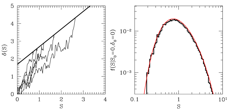
Figure 14: Monte Carlo solution for the first-crossing distribution of a linear barrier with $\beta=1$, $B(S)=\delta_{\mathrm{c}}+S$. The left panel shows a sample of five $\delta(S)$ trajectories that cross the linear threshold. The thin lines are the five trajectories and the thick line is the linear barrier. The histogram in the right panel shows the tabulated first-crossing distribution constructed from $10^{5}$ trajectories. The thin line shows the analytic solution to the first-crossing distribution from Eq. (70). It is clear that the Monte Carlo procedure reproduces the analytic result in the case of the linear barrier.

It can sometimes be useful to consider more general barrier shapes. For example, Furlanetto et al. Furlanetto et al. (2004) used a barrier with a more complicated shape to model the sizes of ionized regions during the epoch of reionization, while Sheth & Tormen Sheth and Tormen (2002) suggested that moving barriers could effectively encapsulate a wide variety of phenomena such as suppression of the collapse of small (low-mass) overdense patches in models where the dark matter is warm. In the latter case, the suppression is due to the non-negligible primordial velocity dispersions of the dark matter particles and the barrier shape could encode the importance of these velocities relative to the depths of the potentials. In this section, I describe two numerical methods to construct the first-crossing distribution for more general barrier shapes.

The most commonly used method to solve for the first-crossing distribution of a barrier of more general shape is direct Monte Carlo construction of the distribution. This method is straightforward. One only needs to compute a large number of $\delta(S)$ trajectories. To construct a trajectory, one computes values of $\delta(S)$ at a discrete set of values of $S$. Maintaining the assumption that the smoothing of the density fluctuation field is performed with a k-space tophat filter, each step is independent and is drawn from Eq. (20) for a step size $\Delta S$. At this point, one only needs to keep track of the value of $S$ at first crossing of the barrier. As with generating halo merger trees, the choice of step size $\Delta S$ is important because all trajectories will be resolved only to within $\Delta S$. The step size must be small enough that a transition above the barrier is rare on any given step. This ensures that multiple barrier crossings are unlikely to be missed.

I give an explicit example of the Monte Carlo method for the linear barrier with $B(S)=\delta_{\mathrm{c}}+S$ in Fig. 14. The left panel shows a sample of five trajectories that cross the linear threshold. Of course, most trajectories do not cross the threshold in the range of $S$ that I show. I have selected five that do and so these trajectories are a biased subsample of the ensemble of all trajectories. The right panel shows the tabulated first-crossing distribution constructed from $10^{5}$ trajectories. It is evident that the Monte Carlo method reproduces the analytic result of the previous section quite well.

Recently, Zhang and Hui Zhang and Hui (2006) described a very useful and elegant method for solving the first-crossing problem for barriers of a very wide range of possible shapes. Zhang & Hui pointed out that the problem can be recast in the form of an integral equation that can be solved by well-known methods.

The first step is to recognize that all trajectories either are included in $\Pi(\delta,S)$ or penetrate the barrier so that

$$\int_{0}^{S}\ f(S^{\prime})\mathrm{d}S^{\prime}+\int_{-\infty}^{B(S)}\ \Pi(\delta,S)\mathrm{d}\delta=1,$$ (73)

where $f(S)$ is the first-crossing distribution and $B(S)$ is the scale-dependent barrier height. If there were no barrier, the distribution of $\Pi(\delta,S)$ would be given by $\Psi(\delta,S)$ from Eq. (20). Therefore, $\Pi(\delta,S)$ should be given by $\Psi(\delta,S)$ minus the trajectories that pierced the barrier at some $S^{\prime}<S$ and migrated downward to $\delta$ by a variance $S$. Thus

$$\Pi(\delta,S)=\Psi(\delta,S)-\int_{0}^{S}\ f(S^{\prime})\Psi(\delta-B(S),S-S^{\prime})\mathrm{d}S^{\prime}.$$ (74)

Taking the derivative of Eq. (73) with respect to $S$ gives an integral relation for $f(S)$ in terms of $\Pi(\delta,S)$ and the barrier shape. Substituting $\Pi(\delta,S)$ from Eq. (74) into this integral relation for $f(S)$ gives

$$f(S)=G(S)+\int_{0}^{S}\ f(S^{\prime})H(S,S^{\prime})\mathrm{d}S^{\prime},$$ (75)

where $G(S)\equiv[B(S)/S-2\mathrm{d}B(S)/\mathrm{d}S]\Psi(B(S),S)$, $H(S,S^{\prime})\equiv[2\mathrm{d}B(S)/\mathrm{d}S-(B(S)-B(S^{\prime}))/(S-S^{\prime})]\Psi(B(S)-B(S^{\prime}),S-S^{\prime})$, and $H(S,S^{\prime})=0$ if $S^{\prime}>S$.

Equation (75) is an integral equation for the first-crossing distribution of $f(S)$. Equation (75) has the variable $S$ as a limit of integration, and the unknown function of interest $f(S)$ both under and outside the integral. This is the form of a Volterra Equation of the second kind. This equation can be solved numerically using standard methods (e.g., Ref. Arfken and Weber (1995)). The first step is to discretize the integral on an interval from $0$ to $S$. The simplest approach is to choose a uniform step in $S$. Let $n=1,2,...,N$, $\Delta S=S/N$, $S_{n}=n\Delta S$, $f_{n}=f(S_{n})$, $G_{n}=G(S_{n})$, and $H_{n}m=H(S_{n},S_{m}-\Delta S/2)$. Then, the integral can be rewritten as

$$\int_{0}^{S_{n}}\ f(S^{\prime})\Psi(\delta-B(S_{n}),S_{n}-S^{\prime})\mathrm{d}S^{\prime}\simeq\frac{\Delta S}{2}\sum_{m=1}^{N}\ H_{nm}[f_{m}+f_{m-1}],$$ (76)

so that

$$f_{n}=\frac{G_{n}\ +\ \Delta S/2(\sum_{m=1}^{n-1}\ H_{nm}[f_{m}+f_{m-1}]\ \ +\ H(n,n)f_{n-1})}{1-(\Delta S/2)H(n,n)}$$ (77)

with the exceptions

$$f_{0} = G_{0}\quad\quad\mathrm{and}$$

$$f_{1} = \frac{G_{1}+(\Delta S/2)H(2,1)[f_{1}+f_{0}]}{1-(\Delta S/2)H(2,2)}.$$

The values $f_{n}$ can be constructed iteratively based on Eq. (77). Utilizing Eq. (77) as a solution for Eq. (75) is generally a more efficient method to obtain a precise estimate for $f(S)$ than computing a large ensemble of trajectories.

As a simple example of this approach, I show the first-crossing distribution of the barrier $B(S)=\delta_{\mathrm{c}}+0.5S^{2}$ in Figure 15. The histogram is the first-crossing distribution constructed from $10^{5}$ Monte Carlo trajectories, while the smooth line is the iterative solution to Eq. (75) in Eq. (77). The two solutions are clearly in good agreement. Note also that the first-crossing distribution declines more rapidly at high $S$ (small mass) than the first-crossing distribution for the linear barrier. This is a natural consequence of the fact that the barrier height grows more rapidly with respect to the variance than in the linear case so that the barrier is even more difficult to penetrate at high $S$.

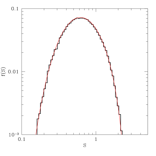
Figure 15: The first-crossing distribution for the quadratic barrier $B(S)=\delta_{\mathrm{c}}+0.5S^{2}$. The histogram is the result of a Monte Carlo construction of the distribution while the smooth, solid line is the iterative solution to the Volterra equation [Eq. (75)] described by Zhang & Hui Zhang and Hui (2006).

IX.3 Correlations Between Scales

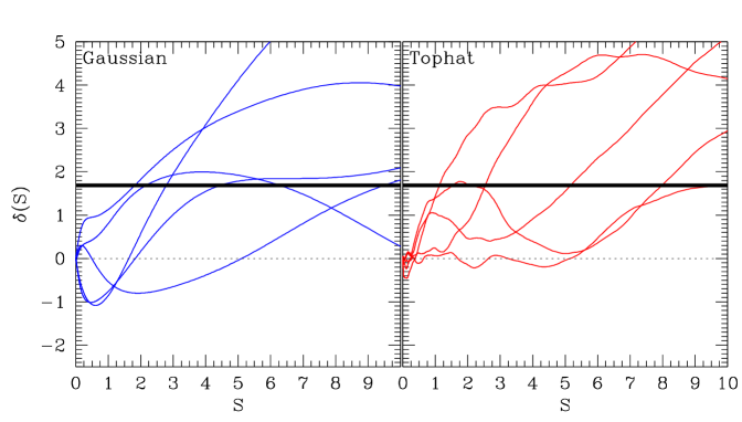
Figure 16: Correlated random walks. The thin, solid lines show five examples of correlated random walks of $\delta(S)$ defined with a Gaussian filter in the left panel and a tophat filter in the right panel. These trajectories were constructed from five integrations of the Langevin equation [Eq. (78)] in each case. The thick line represents a threshold at $\delta=\delta_{\mathrm{c}}$. The trajectories in this figure have been selected to pierce the barrier at $S<10$ which is why they all tend to lie in the upper half plane. Notice that these trajectories vary smoothly, unlike the uncorrelated case.

As I described in § IV, the standard implementation of the excursion set theory makes use of a density contrast field filtered with a k-space tophat window function. This choice of a filter that is local in Fourier space requires that the mass that collapses onto a halo is not local in configuration space. In fact, the previous sentence understates the issue. In § IV, I noted that the use of the sharp k-space filter represents something of a problem because the sharp k-space window is difficult to associate with any particular mass because its volume diverges. However, once some method for assigning mass to a filter scale is decided upon, the use of the sharp k-space filter also has an important implication for the properties of halos. In the case of a sharp k-space window function, the transitions between different smoothed densities are independent Gaussian random variables as in Eq. (20). This implies that the formation histories of halos are completely unrelated to their local environments because in the excursion set formalism a halo of mass $M$ has $\delta(S)=\delta_{\mathrm{c}}$ at $S=S(M)$ while all steps away from this value are independent of each other.

Though the effects are small, several studies have recently pointed out that the formation histories of halos in cosmological numerical simulations are correlated with their environments Sheth and Tormen (2004); Gao et al. (2005); Wechsler et al. (2006); Wetzel et al. (2006) as are internal properties of halos Wechsler et al. (2006); Wetzel et al. (2006); Maccio’ et al. (2006). The implication of these studies is that correlations between scales cannot be neglected completely. Though the impact of these effects on observable quantities has not been thoroughly explored, the first observation of such an effect was recently presented by Berlind et al. Berlind et al. (2006).

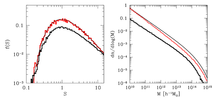
Figure 17: The first-crossing distribution of the smoothed density field defined with a Gaussian window function. The left panel shows the first-crossing distribution explicitly. First the smooth, upper line is the analytic distribution for the sharp k-space window function given in Eq. (32). The upper histogram shows the first-crossing distribution constructed by integrating the Langevin equation for this case and demonstrates that the two solutions are in good agreement. The lower histogram is the first-crossing distribution for the smoothed density field defined with a Gaussian window function. The right panel shows mass functions. The smooth line is the standard excursion set mass function. The lower histogram shows the mass function of halos using the Gaussian first-crossing distribution from the left panel and the $S(M)$ relationship for a Gaussian filter function. The upper histogram shows the mass function constructed from the Gaussian first-crossing distribution of the left panel but using the $S(M)$ relation for a real-space tophat window function. The difference between the two histograms represents the effect of the different mass definitions with a fixed first-crossing distribution.

Along other lines Sheth & Tormen Sheth and Tormen (2002), attempted to determine whether or not their conditional mass functions were in error because of an incomplete treatment of ellipsoidal collapse and concluded that a more detailed treatment of ellipsoidal collapse could not explain the failures of their model to predict conditional mass functions and density-dependent mass functions. They reasoned that because the worst failures occurred in high-density regions and for conditional mass functions at small lookback times and large mass ratios, the deficiency may be due to the neglect of correlations between different scales. The reasoning is as follows. Consider the specific example of the conditional mass function. To compute the conditional mass function, two smoothing scales are necessary. One scale describes the parent object while the other scale describes the progenitor halo at some earlier time. At high mass ratios and small lookback times, the two smoothing scales are quite similar so one might expect correlations to be important. However, in the low-mass-ratio regime where the progenitors are much smaller than the parent halo, the two smoothing scales are very different so that it might not be surprising for correlations between these very different scales to be relatively less important.

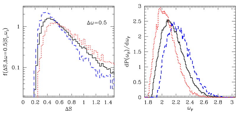
Figure 18: The dependence of halo formation times on halo environment in the excursion set theory. The figure shows results derived from trajectories of $\delta(S)$ defined using a Gaussian window function. The left panel shows the conditional probability for making a first crossing of a barrier of height $\omega=\delta_{\mathrm{c}}+\Delta\omega$ with $\Delta\omega=0.5$, given that the first crossing of the barrier $\omega_{\mathrm{i}}=\delta_{\mathrm{c}}$ occurred in the interval $1.3\leq S_{\mathrm{i}}\leq 1.4$. This corresponds to a mass range $1.8\leq M/[10^{13}\ h^{-1}\mathrm{M}_{\odot}]\leq 2.2$. The solid histogram shows the full conditional probability distribution derived from $10^{5}$ such trajectories. The dotted histogram shows the conditional probability derived from the quartile of trajectories that have the highest smoothed densities on a scale of $R_{\mathrm{env}}=10\ h^{-1}\mathrm{Mpc}$. For the purposes of this exercise, the smoothed density on a scale of $R_{\mathrm{env}}$ serves to define the environment. The dashed histogram shows the conditional probability from the quartile of trajectories with the smallest smoothed densities on a scale of $R_{\mathrm{env}}$. The right panel shows the distributions of formation times (in terms of the variable $\omega_{\mathrm{F}}$) derived from these trajectories. Again, the solid histogram shows the mean distribution of formation times for all halos, the dotted histogram shows the distribution of formation times for the quartile of halos with the highest large-scale densities, and the dashed histogram shows the formation time distribution for the quartile of halos in the lowest density environments. Notice that at fixed halo mass, halos with low large-scale densities typically form earlier (at higher $\omega_{\mathrm{F}}$) than halos that reside in regions that are overdense on large scales.

Correlations between scales can be incorporated into the excursion set approach simply by modifying the window function. Any window function other than a sharp k-space window will result in walks with steps that are correlated to some degree. In the case of correlated walks, Eq. (21) no longer applies and so the results of § IV are not valid. For correlated walks, the $f(S)\mathrm{d}S$ distribution must be computed by integrating numerically a Langevin equation as described in the seminal work of Bond et al. in Ref. Bond et al. (1991).

The Brownian motion of a particle can be treated by considering the acceleration of the particle as due to a fluctuating stochastic force $\vec{F}(t)$. The Langevin equation for the particle motion is $\mathrm{d}\vec{v}/\mathrm{d}t=\vec{F}(t)$, where $\vec{v}$ is the particle velocity (for example, return to the review of Chandrasekhar in Ref. Chandrasekhar (1943)). In a similar way, the trajectory $\delta(S)$ experiences a series of stochastic inputs from specific realizations of the different Fourier modes of the density field. The trajectory for the smoothed density field obeys

$$\frac{\partial\delta(S)}{\partial\ln k}=Q(\ln k)W(k;R_{\mathrm{W}}),$$ (78)

where the variance $S$ and the smoothing scale $R_{\mathrm{W}}$ are related through Eq. (14) as usual. The “stochastic force” in this case is $Q(\ln k)$ which is a Gaussian random variable with zero mean and a variance of

$$\langle Q^{2}(\ln k)\rangle=\frac{\mathrm{d}S}{\mathrm{d}\ln k}=\Delta^{2}(k).$$ (79)

A large number of trajectories can be built up numerically by summing a large number of realizations of the stochastic forces. The algorithm is to select $Q(\ln k)$ on a grid of wavenumbers, to apply the smoothing to each $Q(\ln k)$ on a grid of smoothing scales, and to sum the contributions of each step in wavenumber to construct each trajectory. As before, the steps in smoothing scale should be sufficiently small that crossing the barrier of interest on any particular interval is unlikely, so it is often most efficient to use a non-uniform grid in resolution scale (e.g., see Ref. Bond et al. (1991)).

Figure 16 gives examples of trajectories with correlated steps computed by integrating numerically the Langevin equation of Eq. (78). The left panel shows trajectories generated using a Gaussian window function and the right panel shows trajectories generated using a tophat window function. The most obvious feature of these trajectories is that they do not exhibit the frenetic variations of the uncorrelated random walks shown in Fig. 2 and Fig. 14. On the contrary, because all of the steps in the trajectory are correlated to some degree, the trajectories are smooth functions of scale.

The first-crossing distribution for a set of trajectories with correlated steps can be constructed numerically by generating a large number of trajectories like those in Figure 16. Figure 17 shows the first-crossing distribution for trajectories defined using a Gaussian window function compared to the standard first-crossing distribution for sharp k-space filtering. In the range of $S$ corresponding to halo masses of interest, the first crossing distribution of trajectories defined relative to a Gaussian window is lower than the standard, sharp k-space result. At large values of the variance ($S\lower 2.58334pt\vbox{\hbox{$\buildrel\textstyle>\over{\sim}\ $}}25$), the first-crossing distribution of the trajectories defined relative to a Gaussian filter overtakes the sharp k-space distribution (these features have been discussed in Ref. Bond et al. (1991)). Recall that translating $f(S)$ into a mass function requires knowledge of the relationship between the variance $S$ and the mass scale $M$. Therefore, comparing $f(S)$ for two different filtering functions does not reflect the differences in the mass function directly because the two different $S(M)$ relations must be accounted for. In the case of the sharp k-space filter, the definition of mass is far from obvious because the filter has a divergent volume associated with it. Standard practice is to use the $S(M)$ relation set by a real-space tophat window function. The right panel of Figure 17 shows the mass function for the Gaussian first-crossing distribution using both the Gaussian window relation for $S(M)$ and the real-space tophat relation for $S(M)$ so that the effect of changing the $S(M)$ relation at fixed $f(S)$ on the mass function is evident.

IX.4 Halo Formation Times and Environment: An Example

The excursion set theory using filters other than the sharp k-space filter has been considered only relatively rarely in the literature, but in light of recent results it is interesting to ask what excursion set theory might say about the relationship between halo properties, such as formation time, and halo environments. One can ask what predictions implementing a window that is localized in configuration space, rather than Fourier space, makes for the relation between, in particular, halo formation histories and large-scale halo environments.

Consider as a concrete example the dependence of halo formation time on environment at fixed halo mass. A simple and physically reasonable way to introduce correlations between the past formation histories of halos and the environments in which halos reside is to consider trajectories of $\delta(S)$ defined using a window function that is localized in configuration space. The logic for determining formation times is precisely the same as that in § VII.3, but the probability distributions must be constructed numerically. I show the result of a simple toy example in Figure 18. The argument is fairly general, but for concreteness, take the specific example of the formation times of $10^{13}\ h^{-1}\mathrm{M}_{\odot}$ halos with environment defined as the smoothed density field on scale of $R_{\mathrm{env}}=10\ h^{-1}\mathrm{Mpc}$, $\delta_{\mathrm{env}}\equiv\delta(R_{\mathrm{W}}=R_{\mathrm{env}})$. The calculation must be constructed numerically from a large ensemble of trajectories so it is necessary to take a bin of halo mass that has finite extent. For this exercise, I consider halos that make a first crossing of the barrier $\delta_{\mathrm{c}}$ between $1.3\leq S_{\mathrm{i}}\leq 1.4$. This corresponds to a mass range of approximately $1.8\lower 2.58334pt\vbox{\hbox{$\buildrel\textstyle<\over{\sim}\ $}}M/[10^{13}\ h^{-1}\mathrm{M}_{\odot}]\lower 2.58334pt\vbox{\hbox{$\buildrel\textstyle<\over{\sim}\ $}}2.2$. This toy model is based on $10^{5}$ trajectories of $\delta(S)$ defined using Gaussian filtering so that the steps of the random walks are correlated.

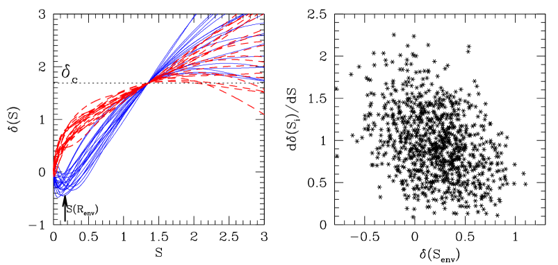
Figure 19: Trajectories exhibiting low and high large-scale densities. The left panel shows twenty randomly-selected trajectories with values of $\delta_{\mathrm{env}}$ in the lowest quartile (solid lines) and $\delta_{\mathrm{env}}$ in the highest quartile (dashed lines). The horizontal, dotted line marks $\delta=\delta_{\mathrm{c}}$ indicating collapse at $z=0$. All trajectories represent halos of nearly identical mass so they cross $\delta_{\mathrm{c}}$ at nearly identical points. The arrow indicates the variance on the length scale $R_{\mathrm{env}}=10\ h^{-1}\mathrm{Mpc}$ which is where the environment measure $\delta_{\mathrm{env}}$ is defined. Notice that trajectories with low large-scale densities tend to rise more rapidly after crossing the threshold at $\delta_{\mathrm{c}}$. The right panel shows a scatter plot of large-scale density contrast $\delta_{\mathrm{env}}$ and the rate of change of $\delta(S)$ at the first-crossing of $\delta_{\mathrm{c}}$ at $S_{\mathrm{i}}$, $\mathrm{d}\delta(S_{\mathrm{i}})/\mathrm{d}S$. The inverse correlation between large-scale density and local rate of increase is evident.

The left panel of Figure 18 shows an explicit example of a conditional probability for crossing a second barrier of height $\omega=\delta_{\mathrm{c}}+\Delta\omega$ with $\Delta\omega=0.5$ in an interval of width $\mathrm{d}S$ about $S$ given a first crossing of the barrier at $\delta_{\mathrm{c}}$ in the range $1.3\leq S_{\mathrm{i}}\leq 1.4$, as specified in the previous paragraph. Also shown in the left panel of Figure 18 is the conditional probability for the quartiles of trajectories with the highest and lowest values of large-scale density $\delta_{\mathrm{env}}$. Notice that the conditional probability $f(\Delta S,\Delta\omega|S_{\mathrm{i}},\omega_{\mathrm{i}})$ is shifted toward lower $\Delta S$ in regions of low density. Trajectories in low-density regions rise more rapidly in the vicinity of the threshold. According to the logic of § VII.3, the consequence of this is that trajectories in low-density regions generally will achieve higher values by the time the smoothing scale decreases to include half of the initial mass. As a direct result, these trajectories will generally correspond to halos with earlier formation times. I show this explicitly in the right panel of Figure 18. This panel shows the distribution of formation times computed from the same set of trajectories for all halos, as well as for the high and low quartiles of $\delta_{\mathrm{env}}$.

Figure 18 shows clearly that introducing correlations between different scales into the excursion set formalism generally leads to halos in dense environments forming later and halos in diffuse environments forming earlier at fixed halo mass. The example of Figure 18 described in the previous paragraphs is fairly specific; however, while the magnitude of this effect varies, the sense of this effect is general and holds for different filter shapes and for $\delta_{\mathrm{env}}$ defined on widely different scales. Interestingly, I have computed the environment-dependent formation time distribution for halos of numerous masses, and the sense of this shift is independent of the mass of halo under consideration.

The generality of this result implies that the excursion set theory with a density field smoothed by a filter that is localized in configuration space will lead to dense regions that preferentially host late-forming halos and vice versa for regions of low density. The result stems from the general fact that the conditional probability $f(\Delta S,\Delta\omega|S_{\mathrm{i}},\omega_{\mathrm{i}})$ is shifted toward low $\Delta S$ in low density regions. There is a simple qualitative explanation for this behavior. All trajectories are required to pass through the point $\omega_{\mathrm{i}}$ at $S_{\mathrm{i}}$ in order to be considered a halo of a particular mass at all. Consider beginning a walk at $S=0$ and $\delta=0$. Trajectories that start so that the large-scale smoothed density is relatively low at some small value of the variance $S$ must rise rapidly in order to cross $\omega_{\mathrm{i}}$ at $S_{\mathrm{i}}$. The steps in the walk or correlated, so that these trajectories typically continue to rise after crossing this threshold. The opposite is true in high-density regions. On average, trajectories that start at low large-scale densities, proceed to pierce subsequent thresholds earlier in the walk than counterpart trajectories with high large-scale densities. This general trend is illustrated in Figure 19 where I show both examples of trajectories in low- and high-density regions and a scatter plot of $\delta_{\mathrm{env}}$ against the rate of change of the trajectories about the crossing of $\delta_{\mathrm{c}}$ at $S_{\mathrm{i}}$, $\mathrm{d}\delta(S_{\mathrm{i}})/\mathrm{d}S$.

The results of this toy model for the environmental dependence of halo formation indicate that the natural expectation of excursion set theory should be that halos in dense environments tend to form relatively later than average, while halos in diffuse environments tend to form relatively earlier than average. Excursion set theory with a constant barrier height predicts this relative trend independent of halo mass. The studies in Refs. Gao et al. (2005); Wechsler et al. (2006); Wetzel et al. (2006); Maccio’ et al. (2006) indicate that low-mass halos ($M\ll M_{\star}$) that form early should be found preferentially in high-density environments and conversely for late-forming halos. This is opposite the excursion set expectation described in the preceding paragraphs. On the contrary, the recent results of Wechsler et al. Wechsler et al. (2006) and Wetzel et al. Wetzel et al. (2006) indicate that in the high-mass regime ($M\lower 2.58334pt\vbox{\hbox{$\buildrel\textstyle>\over{\sim}\ $}}M_{\star}$), it is indeed the late-forming halos that are preferentially located in dense environments.

Wang et al. Wang et al. (2006) have recently studied the origin of the link between formation time and environment using a cosmological numerical simulation. These authors found that low-mass halos that form early are preferentially in dense environments, in agreement with previous work. More interestingly, Wang et al. continued to show that the accretion of matter onto small halos in dense environments is cut off prematurely (relative to excursion set expectations) due to tidal interactions and heating of the ambient environment by significantly more massive neighbors. The low-mass halos are forced to be early formers because their late accretion is eliminated in a competition with massive neighbors. Wang et al. propose this as the origin of the environment-dependent formation times measured in previous numerical studies. Finally, Ref. Wang et al. (2006) went on to show that this competition-limited growth is not important for high-mass halos.

It is interesting to conjecture that the prediction of the excursion set theory and the study by Wang et al. Wang et al. (2006) can be combined into a global picture that explains environment-dependent formation times at all mass scales. In such a scenario, the statistics of overdense patches in the primordial density contrast field would favor a bias toward late halo formation in dense regions. In the high-mass regime, halo growth would not be limited by competition in any meaningful way, so this bias would persist in the sense seen by Ref. Wechsler et al. (2006) and Ref. Wetzel et al. (2006) for high-mass halos in numerical simulations. However, in the low-mass regime, competition would stifle halo growth, forcing small halos in dense environments to be early formers. This gives rise to the bias of small halos in dense regions to be preferentially early formers.

To my knowledge, the issues mentioned in this section have not been addressed in any adequate way at present. The model I have given here is an incomplete toy model intended to illustrate the method for generalizing the excursion set predictions and to indicate the sense of the effect that excursion set theory predicts. A more detailed exploration of these points is an interesting undertaking, but is well beyond the scope of this review.

IX.5 The PINOCCHIO Algorithm

In closing, I would like to point toward another tool for estimating halo mass functions and formation histories quickly and accurately. This is the publicly-available PINOCCHIO code developed by P. Monaco and collaborators  Monaco et al. (2002a, b); Taffoni et al. (2002)^,. (A similar tool that can be used to generate mock catalogs of halos rapidly is PTHalos developed by Scoccimarro and Sheth Scoccimarro (1998); Scoccimarro and Sheth (2002)) The great value of the PINOCCHIO code is that it is considerably less computationally expensive than a cosmological N-body simulation but predicts halo properties and formation histories that are in better agreement with N-body results relative to the simple excursion set approach (for a recent example see Ref. Li et al. (2005)).

Briefly, the PINOCCHIO code uses an algorithm for identifying halos and halo properties such as mass, velocity, angular momentum, in particular realizations of the linear density field. The PINOCCHIO code also contains a parameterized algorithm for building filamentary structures in the density field and for generating the merging histories of halos. PINOCCHIO creates a particle-based realization of the linear density field in a manner similar to standard N-body simulations. PINOCCHIO then computes the approximate evolution of mass elements using a particular truncation of third order Lagrangian perturbation theory (for example, first order Lagrangian perturbation theory constitutes the well-known Zel’dovich Approximation used to initialize most N-body simulations). As PINOCCHIO is perturbative, the computation progresses at a fraction of the computational effort of an N-body simulation. PINOCCHIO groups mass elements together into halos using an orbit-crossing condition. When the orbits of two mass elements coincide, Lagrangian perturbation theory breaks down because the mapping from Eulerian position to Lagrangian position becomes multi-valued and the density is infinite. At this point, the mass elements are grouped together into a halo (or perhaps a filament) in analogy with collapse to a point in the evolution of a spherical tophat overdensity.

The development of the algorithm and the PINOCCHIO code involves a great deal of detail and is well-beyond the scope of this review. However, this development is well-documented and the references above provide a good starting point for understanding the calculation.

Acknowledgments

I would like to thank Jeremy Tinker for making is numerical data available to me for this review. I thank James Bullock, Neal Dalal, Anatoly Klypin, Andrey Kravtsov, Savvas Koushiappas, Brant Robertson, Eduardo Rozo, Douglas Rudd, Frank van den Bosch, Risa Wechsler, and David Weinberg for useful discussions and/or comments on the manuscript. This review is based on notes for lectures given at the Sixth Summer School of the Helmholtz Institute for Supercomputational Physics on Supercomputational Cosmology. The Summer School is funded by the Ministry for Science, Research, and Culture Brandenburg. I would like to thank the organizer of the Summer School on Supercomputational Cosmology, Anatoly Klypin, for inviting me to give these lectures. I thank Anatoly Klypin, Andrey Kravtsov and Francisco Prada for encouraging me to expand them to the current review. I thank the Astrophysical Institute Potsdam for hospitality during my stay. This work was funded by the Kavli Institute for Cosmological Physics at the University of Chicago, by the National Science Foundation under grant NSF PHY 0114422, and by the National Science Foundation through the Astronomy and Astrophysics Postdoctoral Fellowship Program under grant AST 0602122.

References

- Press and Schechter (1974) W. H. Press and P. Schechter, Astrophys. J. 187, 425 (1974).
- Somerville and Kolatt (1999) R. S. Somerville and T. S. Kolatt, MNRAS 305, 1 (1999).
- Cole et al. (2000) S. Cole, C. G. Lacey, C. M. Baugh, and C. S. Frenk, MNRAS 319, 168 (2000).
- Somerville and Primack (1999) R. S. Somerville and J. R. Primack, MNRAS 310, 1087 (1999), eprint astro-ph/9802268.
- Kauffmann and Haehnelt (2000) G. Kauffmann and M. Haehnelt, MNRAS 311, 576 (2000), eprint astro-ph/9906493.
- Neistein et al. (2006) E. Neistein, F. C. van den Bosch, and A. Dekel, ArXiv Astrophysics e-prints (2006), eprint astro-ph/0605045.
- Zentner and Bullock (2003) A. R. Zentner and J. S. Bullock, ApJ 598, 49 (2003).
- Benson et al. (2004) A. J. Benson, C. G. Lacey, C. S. Frenk, C. M. Baugh, and S. Cole, MNRAS 351, 1215 (2004), eprint astro-ph/0307298.
- Koushiappas et al. (2004) S. M. Koushiappas, A. R. Zentner, and T. P. Walker, Phys. Rev. D 69, 043501 (2004), eprint astro-ph/0309464.
- Zentner et al. (2005) A. R. Zentner, A. Berlind, J. S. Bullock, A. Kravtsov, and R. H. Wechsler, Astrophys. J. , 624, 505 (2005).
- Peñarrubia and Benson (2005) J. Peñarrubia and A. J. Benson, MNRAS 364, 977 (2005), eprint astro-ph/0412370.
- Taylor and Babul (2005a) J. E. Taylor and A. Babul, MNRAS 364, 515 (2005a).
- Taylor and Babul (2005b) J. E. Taylor and A. Babul, MNRAS 364, 535 (2005b), eprint astro-ph/0410049.
- Monaco et al. (2002a) P. Monaco, T. Theuns, and G. Taffoni, MNRAS 331, 587 (2002a).
- Monaco et al. (2002b) P. Monaco, T. Theuns, G. Taffoni, F. Governato, T. Quinn, and J. Stadel, MNRAS 564, 8 (2002b).
- Taffoni et al. (2002) G. Taffoni, P. Monaco, and T. Theuns, MNRAS 333, 623 (2002).
- Bardeen et al. (1986) J. M. Bardeen, J. R. Bond, N. Kaiser, and A. S. Szalay, Astrophys. J. 304, 15 (1986).
- Bond et al. (1991) J. R. Bond, S. Cole, G. Efstathiou, and N. Kaiser, Astrophys. J. 379, 440 (1991).
- Lacey and Cole (1993) C. Lacey and S. Cole, MNRAS 262, 627 (1993).
- Lacey and Cole (1994) C. Lacey and S. Cole, MNRAS 271, 676 (1994), eprint astro-ph/9402069.
- Sheth and Lemson (1999) R. K. Sheth and G. Lemson, MNRAS 305, 946 (1999).
- Wax (1954) N. Wax, Selected Papers on Noise and Stochastic Processes (New York: Dover Publication, 1954, edited by Wax, Nelson, 1954).
- Chandrasekhar (1943) S. Chandrasekhar, Rev. Mod. Phys. 15, 2 (1943).
- Rice (1944) S. O. Rice, Bell Systems Tech. J., Volume 23, p. 282-332 23, 282 (1944).
- Rice (1945) S. O. Rice, Bell Systems Tech. J., Volume 24, p. 46-156 24, 46 (1945).
- Eisenstein and Hu (1999) D. J. Eisenstein and W. Hu, Astrophys. J. 511, 5 (1999), eprint astro-ph/9710252.
- Williams et al. (1991) B. G. Williams, A. F. Heavens, J. A. Peacock, and S. F. Shandarin, MNRAS 250, 458 (1991).
- Carroll et al. (1992) S. M. Carroll, W. H. Press, and E. L. Turner, ARAA 30, 499 (1992).
- Bildhauer et al. (1992) S. Bildhauer, T. Buchert, and M. Kasai, A & A 263, 23 (1992).
- Epstein (1983) R. A. Epstein, MNRAS 205, 207 (1983).
- Peacock and Heavens (1990) J. A. Peacock and A. F. Heavens, MNRAS 243, 133 (1990).
- Bower (1991) R. J. Bower, MNRAS 248, 332 (1991).
- Adler (1981) R. J. Adler, The Geometry of Random Fields (The Geometry of Random Fields, Chichester: Wiley, 1981, 1981).
- Sheth and Tormen (1999) R. K. Sheth and G. Tormen, MNRAS 308, 119 (1999).
- Jenkins et al. (2001) A. Jenkins, C. S. Frenk, S. D. M. White, J. M. Colberg, S. Cole, A. E. Evrard, H. M. P. Couchman, and N. Yoshida, MNRAS 321, 372 (2001).
- Kaiser (1984) N. Kaiser, ApJL 284, L9 (1984).
- Efstathiou et al. (1988) G. Efstathiou, C. S. Frenk, S. D. M. White, and M. Davis, MNRAS 235, 715 (1988).
- Mo and White (1996) H. J. Mo and S. D. M. White, MNRAS 282, 347 (1996).
- Seljak and Warren (2004) U. Seljak and M. S. Warren, MNRAS 355, 129 (2004), eprint astro-ph/0403698.
- Cole and Kaiser (1989) S. Cole and N. Kaiser, MNRAS 237, 1127 (1989).
- Sheth et al. (2001) R. K. Sheth, H. J. Mo, and G. Tormen, MNRAS 323, 1 (2001).
- Sheth and Tormen (2002) R. K. Sheth and G. Tormen, MNRAS 329, 61 (2002).
- Scherrer and Bertschinger (1991) R. J. Scherrer and E. Bertschinger, Astrophys. J. 381, 349 (1991).
- Seljak (2000) U. Seljak, MNRAS 318, 203 (2000).
- Ma and Fry (2000) C.-P. Ma and J. N. Fry, Astrophys. J. 543, 503 (2000).
- Peacock and Smith (2000) J. A. Peacock and R. E. Smith, MNRAS 318, 1144 (2000).
- Berlind and Weinberg (2002) A. A. Berlind and D. H. Weinberg, Astrophys. J. 575, 587 (2002).
- Icke (1984) V. Icke, MNRAS 206, 1 (1984).
- Bertschinger (1985) E. Bertschinger, ApJS 58, 1 (1985).
- van de Weygaert and Van Kampen (1993) R. van de Weygaert and E. Van Kampen, MNRAS 263, 481 (1993).
- Sheth and van de Weygaert (2004) R. K. Sheth and R. van de Weygaert, MNRAS 350, 517 (2004).
- Blumenthal et al. (1992) G. R. Blumenthal, L. Da Costa, D. S. Goldwirth, M. Lecar, and T. Piran, Astrophys. J. 388, 234 (1992).
- Furlanetto and Piran (2005) S. Furlanetto and T. Piran, MNRAS, in press (2005), eprint arXiv:astro-ph/0509148.
- Cole and Kaiser (1988) S. Cole and N. Kaiser, MNRAS 233, 637 (1988).
- Cole (1991) S. Cole, Astrophys. J. 367, 45 (1991).
- Kauffmann et al. (1993) G. Kauffmann, S. D. M. White, and B. Guiderdoni, MNRAS 264, 201 (1993).
- Sheth (1996) R. K. Sheth, MNRAS 281, 1277 (1996).
- Sheth and Pitman (1997) R. K. Sheth and J. Pitman, MNRAS 289, 66 (1997).
- White (1996) S. D. M. White, in Cosmology and Large Scale Structure, edited by R. Schaeffer, J. Silk, M. Spiro, and J. Zinn-Justin (1996), pp. 349–+.
- Gelb and Bertschinger (1994) J. M. Gelb and E. Bertschinger, Astrophys. J. 436, 467 (1994), eprint astro-ph/9408028.
- Jing (1998) Y. P. Jing, ApJL 503, L9+ (1998), eprint astro-ph/9805202.
- Tormen (1998) G. Tormen, MNRAS 297, 648 (1998), eprint astro-ph/9802290.
- Wechsler et al. (2002) R. H. Wechsler, J. S. Bullock, J. R. Primack, A. V. Kravtsov, and A. Dekel, Astrophys. J. 568, 52 (2002).
- Sheth and Tormen (2004) R. K. Sheth and G. Tormen, MNRAS 350, 1385 (2004).
- Benson et al. (2005) A. J. Benson, M. Kamionkowski, and S. H. Hassani, MNRAS 357, 847 (2005), eprint astro-ph/0407136.
- Li et al. (2005) Y. Li, H. J. Mo, and F. C. van den Bosch, MNRASSubmitted, astro-ph/0510372 (2005), eprint astro-ph/0510372.
- Sheth (1998) R. K. Sheth, MNRAS 300, 1057 (1998).
- Monaco (1995) P. Monaco, Astrophys. J. 447, 23 (1995), eprint astro-ph/9406029.
- Bond and Myers (1996) J. R. Bond and S. T. Myers, ApJS 103, 1 (1996).
- Monaco (1997a) P. Monaco, MNRAS 287, 753 (1997a), eprint astro-ph/9606027.
- Monaco (1997b) P. Monaco, MNRAS 290, 439 (1997b), eprint astro-ph/9606029.
- Audit et al. (1997) E. Audit, R. Teyssier, and J.-M. Alimi, å 325, 540 (1997).
- Lee and Shandarin (1998) J. Lee and S. Shandarin, Astrophys. J. 500, 14 (1998).
- Furlanetto et al. (2004) S. Furlanetto, M. Zaldarriaga, and L. Hernquist, Astrophys. J. 613, 1 (2004).
- Zhang and Hui (2006) J. Zhang and L. Hui, Astrophys. J. 641, 641 (2006), eprint astro-ph/0508384.
- Arfken and Weber (1995) G. B. Arfken and H. J. Weber, Materials and Manufacturing Processes (1995).
- Gao et al. (2005) L. Gao, V. Springel, and S. D. M. White, MNRAS 363, L66 (2005).
- Wechsler et al. (2006) R. H. Wechsler, A. R. Zentner, J. S. Bullock, A. V. Kravtsov, and B. Allgood, ApJ, In Press (astro-ph/0512416) (2006).
- Wetzel et al. (2006) A. R. Wetzel, J. D. Cohn, M. White, D. E. Holz, and M. S. Warren, ArXiv Astrophysics e-prints (2006), eprint astro-ph/0606699.
- Maccio’ et al. (2006) A. V. Maccio’, A. A. Dutton, F. C. van den Bosch, B. Moore, D. Potter, and J. Stadel, MNRASSubmitted, astro-ph/0608157 (2006), eprint astro-ph/0608157.
- Berlind et al. (2006) A. A. Berlind, E. Kazin, M. R. Blanton, S. Pueblas, R. Scoccimarro, and D. W. Hogg, ArXiv Astrophysics e-prints (2006), eprint astro-ph/0610524.
- Wang et al. (2006) H. Y. Wang, H. J. Mo, and Y. P. Jing, MNRAS, Submitted (astro-ph/0608690) (2006).
- Scoccimarro and Sheth (2002) R. . Scoccimarro and R. K. Sheth, MNRAS 329, 629 (2002).
- Scoccimarro (1998) R. Scoccimarro, MNRAS 299, 1097 (1998).