The Radio-Loud Fraction of Quasars is a Strong Function of Redshift and Optical Luminosity

Abstract

Using a sample of optically-selected quasars from the Sloan Digital Sky Survey, we have determined the radio-loud fraction (RLF) of quasars as a function of redshift and optical luminosity. The sample contains more than 30,000 objects and spans a redshift range of $0<z\leqslant 5$ and a luminosity range of $-30\leqslant M_{i}<-22$. We use both the radio-to-optical flux ratio ($R$ parameter) and radio luminosity to define radio-loud quasars. After breaking the correlation between redshift and luminosity due to the flux-limited nature of the sample, we find that the RLF of quasars decreases with increasing redshift and decreasing luminosity. The relation can be described in the form of log(RLF/(1–RLF)) $=b_{0}+b_{z}\log(1+z)+b_{M}(M_{2500}+26)$, where $M_{2500}$ is the absolute magnitude at rest-frame 2500 Å, and $b_{z}$, $b_{M}<0$. When using $R>10$ to define radio-loud quasars, we find that $b_{0}=-0.132\pm 0.116$, $b_{z}=-2.052\pm 0.261$, and $b_{M}=-0.183\pm 0.025$. The RLF at $z=0.5$ declines from 24.3% to 5.6% as luminosity decreases from $M_{2500}=-26$ to $M_{2500}=-22$, and the RLF at $M_{2500}=-26$ declines from 24.3% to 4.1% as redshift increases from 0.5 to 3, suggesting that the RLF is a strong function of both redshift and luminosity. We also examine the impact of flux-related selection effects on the RLF determination using a series of tests, and find that the dependence of the RLF on redshift and luminosity is highly likely to be physical, and the selection effects we considered are not responsible for the dependence.

1 Introduction

Although quasars were first discovered by their radio emission (e.g. Matthews & Sandage, 1963; Schmidt, 1963), it was soon found that the majority of quasars were radio-quiet (e.g. Sandage, 1965). Quasars are often classified into two broad categories, radio-loud and radio-quiet, based on their radio properties. There is mounting evidence that the distribution of radio-to-optical flux ratio for optically-selected quasars is bimodal (e.g. Kellermann et al., 1989; Miller, Peacock, & Mead, 1990; Visnovsky et al., 1992; Ivezić et al., 2002), although the existence of the bimodality has been questioned (e.g. Cirasuolo et al., 2003, but see also Ivezić et al. (2004a) for a response). Radio-loud and radio-quiet quasars are probably powered by similar physical mechanisms (e.g. Barthel, 1989; Urry & Padovani, 1995), and their radio properties are also correlated with host galaxy properties, central black hole masses, black hole spins, and accretion rates (e.g. Baum et al., 1995; Urry & Padovani, 1995; Best et al., 2005). Radio-loud quasars are likely to reside in more massive galaxies (e.g. Peacock, Miller, & Longair, 1986; Best et al., 2005), and harbor more massive central black holes (e.g. Laor, 2000; Lacy et al., 2001; McLure & Jarvis, 2004), than do radio-quiet quasars.

Roughly 10%$-$20% of all quasars are radio-loud (e.g. Kellermann et al., 1989; Urry & Padovani, 1995; Ivezić et al., 2002). However, the radio-loud fraction (RLF) of quasars may depend on redshift and optical luminosity. Some studies have found that the RLF tends to drop with increasing redshift (e.g. Peacock, Miller, & Longair, 1986; Miller, Peacock, & Mead, 1990; Visnovsky et al., 1992; Schneider et al., 1992) and decreasing luminosity (e.g. Padovani, 1993; Goldschmidt et al., 1999; Cirasuolo et al., 2003), or evolves non-monotonically with redshift and luminosity (e.g. Hooper et al., 1995; Bischof & Becker, 1997), while others showed that the RLF does not differ significantly with redshift (e.g. Goldschmidt et al., 1999; Stern et al., 2000; Cirasuolo et al., 2003) or luminosity (e.g. Bischof & Becker, 1997; Stern et al., 2000).

From a sample of 4472 quasars from the Sloan Digital Sky Survey (SDSS; York et al., 2000), Ivezić et al. (2002) found that the RLF is independent of both redshift and optical luminosity when using marginal distributions of the whole sample; however, they noted that the approximate degeneracy between redshift and luminosity in the SDSS flux-limited sample may cause individual trends in redshift and luminosity to appear to cancel. By stacking the images of the Faint Images of the Radio Sky at Twenty-cm survey (FIRST; Becker, White, & Helfand, 1995), White et al. (2006) were able to probe the radio sky into nanoJansky regime. They found that the median radio loudness of SDSS-selected quasars is a declining function with optical luminosity. After correcting for this effect, they claimed that the median radio loudness is independent of redshift. In this paper we use a sample of more than 30,000 optically-selected quasars from the SDSS, and break the redshift-luminosity dependence to study the evolution of the RLF. We will find that there are indeed strong trends in redshift and luminosity, and that they do in fact roughly cancel in the marginal distributions.

In $\S$2 of this paper, we present our quasar sample from the SDSS. In $\S$3 we derive the RLF of quasars as a function of redshift and optical luminosity. We examine the effects of K corrections and sample incompleteness in $\S$4, and we give the discussion and summary in $\S$5 and $\S$6, respectively. Throughout the paper we use a $\Lambda$-dominated flat cosmology with H₀ = 70 km s^-1 Mpc^-1, $\Omega_{m}$ = 0.3, and $\Omega_{\Lambda}$ = 0.7 (e.g. Spergel et al., 2006).

2 The SDSS quasar sample

The SDSS (York et al., 2000) is an imaging and spectroscopic survey of the sky using a dedicated wide-field 2.5m telescope (Gunn et al., 2006). The imaging is carried out in five broad bands, $ugriz$, spanning the range from 3000 to 10,000 Å (Fukugita et al., 1996; Gunn et al., 1998). From the resulting catalogs of objects, quasar candidates (Richards et al., 2002) are selected for spectroscopic follow-up. Spectroscopy is performed using a pair of double spectrographs with coverage from 3800 to 9200 Å, and a resolution $\lambda/\Delta\lambda$ of roughly 2000. The SDSS quasar survey spectroscopically targets quasars with $i<19.1$ at low redshift ($z\leqslant 3$) and $i<20.2$ at high redshift ($z\geqslant 3$). The low-redshift selection is performed in $ugri$ color space, and the high-redshift selection is performed in $griz$ color space. In addition to the optical selection, a SDSS object is also considered to be a primary quasar candidate if it is an optical point source located within $2\farcs 0$ of a FIRST radio source. All SDSS magnitudes mentioned in this paper have been corrected for Galactic extinction using the maps of Schlegel, Finkbeiner, & Davis (1998).

The sample we used is from the SDSS Data Release Three (DR3; Abazajian et al., 2005). The quasar catalog of the DR3 consists of 46,420 objects with luminosities larger than $M_{i}=-22$ (Schneider et al., 2005). The area covered by the catalog is about 3732 deg². We reject 4683 objects that are not covered by the FIRST survey, and we only use the quasars which were selected on their optical colors (i.e., the quasars with one or more of the following target selection flags: QSO_HIZ, QSO_CAP and QSO_SKIRT; see Richards et al. 2002) to avoid the bias introduced by the FIRST radio selection. The final sample consists of 31,835 optically-selected quasars from the SDSS DR3 catalog, and covers a redshift range of $0<z\leqslant 5$ and a luminosity range of $-30\leqslant M_{i}<-22$.

To include both core-dominated (hereafter FR1) and lobe-dominated (hereafter FR2) quasars, we match our sample to the FIRST catalog (White et al., 1997) with a matching radius 30$\arcsec$. For the quasars that have only one radio source within 30$\arcsec$, we match them again to the FIRST catalog within 5$\arcsec$ and classify the matched ones as FR1 quasars. The quasars that have multiple entries within 30$\arcsec$ are classified as FR2 quasars. The sample contains 2566 FIRST-detected quasars, including 1944 FR1 quasars and 622 FR2 quasars.

We use the integrated flux density ($f_{int}$) in the FIRST catalog to describe the 20 cm radio emission. The total radio flux density of each FR2 quasar is determined using all of the radio components within 30$\arcsec$. We note that we have excluded those FR2 quasars whose separations between lobes are greater than 1$\arcmin$. In fact, FR2 quasars represent a small fraction of the SDSS DR3 catalog, and FR2 quasars with diameters greater than 1$\arcmin$ are even rarer (de Vries, Becker, & White, 2006). These numbers are too small to affect the statistics below. Therefore we do not use more sophisticated procedures (e.g. Ivezić et al., 2002; de Vries, Becker, & White, 2006) to select FR2 quasars.

3 RLF of quasars as a function of redshift and optical luminosity

We define a radio-loud quasar based on its $R$ parameter, the rest-frame ratio of the flux density at 6 cm (5 GHz) to the flux density at 2500 Å (e.g. Stocke et al., 1992). For a given quasar, we calculate its observed flux density $f_{6cm}$ at rest-frame 6 cm from $f_{int}$ (if detected) assuming a power-law slope of $-0.5$ (e.g. Ivezić et al., 2004b); and we determine its observed flux density $f_{2500}$ at rest-frame 2500 Å by fitting a model spectrum to the SDSS broadband photometry (Fan et al., 2001; Jiang et al., 2006; Richards et al., 2006). The model spectrum is a power-law continuum ($f_{\nu}=A{\nu}^{\alpha}$) plus a series of emission lines extracted from the quasar composite spectrum (Vanden Berk et al., 2001). We integrate the model spectrum over the redshifted SDSS bandpasses to compare with the observed magnitudes. The parameters $\alpha$ and $A$ are determined by minimizing the differences between the model spectrum magnitudes $m^{model}$ and the SDSS photometry $m^{obs}$:

$${\chi}^{2}=\sum\left(\frac{m^{model}_{i}-m^{obs}_{i}}{\sigma^{obs}_{i}}\right)^{2},$$ (1)

where $\sigma^{obs}_{i}$ is the estimated SDSS photometry error in the $i^{\rm th}$ SDSS filter. We constrain $\alpha$ to be in the range $-1.1<\alpha<0.1$, and only use the bands that are not dominated by Lyman forest absorption systems. Finally $f_{2500}$ is computed from the power-law continuum using the best-fit values of $\alpha$ and $A$, and the radio loudness $R$ is obtained by

$$R=f_{6cm}/f_{2500}.$$ (2)

The absolute magnitude $M_{2500}$ at rest-frame 2500 Å is calculated from $f_{2500}$.

The FIRST survey has a 5$\sigma$ peak flux density limit of about 1.0 mJy (Becker, White, & Helfand, 1995), although this limit is not perfectly uniform across the sky. For a quasar detected by FIRST, we determine the relevant limit directly from the FIRST catalog, while for a quasar undetected by FIRST, we measure the limit at the position of the nearest radio source (usually within $10\arcmin$). We find that the median value of the limits is 0.98 mJy, which has already included the effect of “CLEAN bias” (Becker, White, & Helfand, 1995; White et al., 1997). Only $\sim 4$% of the quasars have limits above 1.1 mJy, so we use 1.1 mJy as the FIRST detection limit for our sample.

Many sources in the FIRST images are resolved. The resolution effect causes FIRST to become more incomplete for extended objects near the detection limit (Becker, White, & Helfand, 1995; White et al., 1997). Furthermore, FR2 quasars are more incomplete than FR1 quasars for integrated flux densities. For example, a double-lobe radio source with two identical components suffers from incompleteness twice as high as a single-component source of the same total flux density. Figure 1 (provided by R. L. White, private communication) shows the FIRST completeness as a function of integrated flux density. The completeness is computed using the observed size distribution and rms values of integrated flux densities from the FIRST survey for SDSS quasars, and has included all effects mentioned above. Quasars with $f_{int}>5$ mJy have a completeness fraction $g_{comp}\approx 1$ (100%); while for a quasar with 1.1 mJy $<f_{int}<$ 5 mJy, its $g_{comp}$ is measured from the curve. To correct for sample incompleteness, we use the weight of $1/g_{comp}$ when we calculate the numbers of radio-loud quasars.

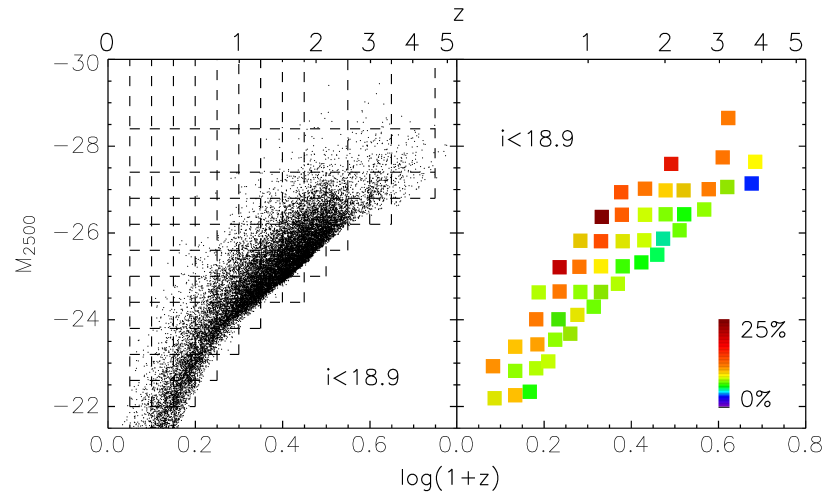
Figure 2: Left panel: Redshift and absolute magnitude distribution for 20,473 quasars with $i<18.9$ in our sample. The $M_{2500}$–$z$ plane is divided into small grids to break the redshift-luminosity dependence. RLFs of quasars are calculated in individual grids. Right panel: The $R$-based RLFs in individual $M_{2500}$–$z$ bins. The square for each subsample is positioned at the median values of $M_{2500}$ and $z$ in that subsample. The RLF of quasars declines with increasing redshift and decreasing luminosity.

When quasars with $R>10$ are defined as radio-loud (e.g. Kellermann et al., 1989), FIRST is able to detect radio-loud quasars down to $i\approx 18.9$ based on Equation 2, the K corrections we applied and the FIRST detection limit of 1.1 mJy. The left panel of Figure 2 shows the redshift and absolute magnitude distribution of our sample.

In flux-limited surveys, redshift and luminosity are artificially correlated, making it difficult to separate the dependence of the RLF on redshift or luminosity. To break this degeneracy, we divide the $M_{2500}$–$z$ plane into small grids. RLFs in individual $M_{2500}$–$z$ grids are calculated and presented as squares in the right panel of Figure 2, where the square for each subsample is located at the median values of $M_{2500}$ and $z$ in that subsample. The RLF declines with increasing redshift and decreasing luminosity. One can see the trend more clearly in Figure 3, in which we plot the RLF in three small redshift ranges and three small magnitude ranges.

We assume a simple relation to model the RLF as a function of redshift and absolute magnitude,

$$\log\left(\frac{RLF}{1-RLF}\right)=b_{0}+b_{z}\log(1+z)+b_{M}(M_{2500}+26),$$ (3)

where $b_{0}$, $b_{z}$ and $b_{M}$ are constants. We use the RLFs calculated from the grids that include more than one radio-loud quasar, and use median values of $z$ and $M_{2500}$ in each grid. Statistical uncertainties are estimated from Poisson statistics. The best fitting results found by regression fit are, $b_{0}=-0.132\pm 0.116$, $b_{z}=-2.052\pm 0.261$, and $b_{M}=-0.183\pm 0.025$. This implies that when RLF $\ll 1$, RLF $\propto(1+z)^{-2.052}L_{opt}^{0.458}$, where $L_{opt}$ is the optical luminosity. The $\chi^{2}$ of this fit is 52.8 for 47 degrees of freedom (DoF), and the confidence levels of $b_{z}$ and $b_{M}$ are shown in Figure 4. The null hypothesis that $b_{z}=0$ and $b_{M}=0$ is rejected at $>5\sigma$ significance. The results are projected onto two-dimensional plots in the left panels of Figure 5, where filled circles are the RLFs calculated from individual grids in Figure 2 and dashed lines are the best fits. The upper panel shows the RLF as a function of redshift after correcting for the luminosity dependence. At $M_{2500}=-26$, the RLF drops from $\sim$24.3% to $\sim$4.1% as the redshift increases from 0.5 to 3. The lower panel shows the RLF as a function of luminosity after correcting for the redshift dependence. At $z=0.5$, the RLF decreases rapidly from $\sim$24.3% to $\sim$5.6% as the luminosity decreases from $M_{2500}=-26$ to $M_{2500}=-22$. Therefore the RLF of quasars is a strong function of both redshift and optical luminosity.

To probe whether the trend seen in Equation 3 is related to the radio-loud criterion adopted, we define a radio-loud quasar if $R$ is greater than 30 instead of 10. In this case FIRST is able to detect radio-loud quasars down to $i\approx 20.0$. We calculate RLFs for the quasars with $i<20.0$ using the same method illustrated in Figure 2, and model the RLF with Equation 3. The best fitting parameters are given in Table 1 and the confidence levels of $b_{z}$ and $b_{M}$ are shown in Figure 4. Figure 5 shows the RLF as a function of redshift and luminosity. The relation gives similar results for both radio-loud criteria. We note that the sample of $i<20.0$ at $z<3$ is not complete since some bins in $M_{2500}$–$z$ space are not sampled by SDSS. However, this incompleteness does not bias our results because we are considering the RLF for optically-selected quasars. Another definition of a radio-loud quasar is based on the radio luminosity of an object (e.g. Peacock, Miller, & Longair, 1986; Miller, Peacock, & Mead, 1990; Hooper et al., 1995; Goldschmidt et al., 1999). As we do for the $R$-based RLF, we use two criteria to define radio-loud quasars: $L_{r}$ (luminosity density at rest-frame 6 cm) $>10^{32}$ ergs s^-1 Hz^-1 and $L_{r}>10^{32.5}$ ergs s^-1 Hz^-1. In the two cases, FIRST is able to detect radio-loud quasars up to $z\sim 2.1$ and 3.5, respectively. We model the RLF using Equation 3 and repeat the analysis. The best fitting results are shown in Table 1, and Figures 4 and 6. The RLF based on $L_{r}$ is correlated with $z$ and $M_{2500}$ in the same manner as the $R$-based criteria.

4 Effects of the K corrections and sample incompleteness

When applying the K corrections, we assumed that the slope of the radio continuum is $-0.5$ and used a model spectrum to determine the optical continuum slope. To investigate the effect of the K corrections, we performed several experiments. First, for a given quasar at $z$, we calculated its $f_{2500}$ and $M_{2500}$ from the magnitude in the SDSS band whose effective wavelength is closest to $2500(1+z)$ Å assuming a slope of $-0.5$ (Test 1). As before, we corrected for the contribution from emission lines. Because the SDSS $ugriz$ photometry covers a wavelength range of 3000 to 10,000 Å, the K corrections for $z<3$ require no extrapolation. Second, we assumed two extreme cases for the radio and optical slopes: in Test 2, we took the optical slope to be 0.0 and the radio slope as $-1.0$, while in Test 3, the optical slope was $-1.0$ and the radio slope was 0.0. The results of the fit to Equation 3 are listed in Table 1. The values of $b_{z}$ and $b_{M}$ recalculated under these tests differ by less than 2$\sigma$ from the original values, and the null hypothesis that $b_{z}=0$ and $b_{M}=0$ is rejected at $>5\sigma$ significance in all these tests. Therefore the effect of the K corrections on our conclusions is small.

We investigated the reliability of the relation described by Equation 3 for different definitions of radio loudness and for luminosities in different optical bands. For example, we defined the $R$ parameter as the rest-frame ratio of the flux density at 6 cm to the flux density at 4400 Å (e.g. Kellermann et al., 1989) instead of 2500 Å, and we repeated the analysis in $\S$3 (Test 4). In Test 5, we determined the RLF as a function of $z$ and $M_{i}$ (instead of $M_{2500}$). $M_{i}$ is the absolute magnitude in the rest-frame $i$ band, and was calculated using the method described in $\S$3. The results are listed in Table 1. In these cases the RLF is still strongly dependent on redshift and luminosity, and the relation described by Equation 3 is not sensitive to the details of how radio loudness is defined.

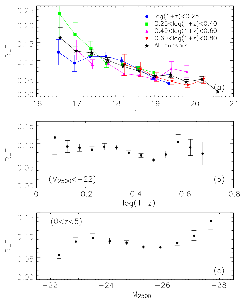
Figure 7: (a): RLF as a function of apparent magnitude $i$ for five redshift bins. The RLF declines with increasing $i$, and the curves for different redshift bins follow the same RLF–$i$ dependence. (b) and (c): Marginal RLF as a function of redshift and luminosity for our sample. The marginal RLF is roughly independent of both redshift and luminosity due to the $M_{2500}$–$z$ degeneracy.

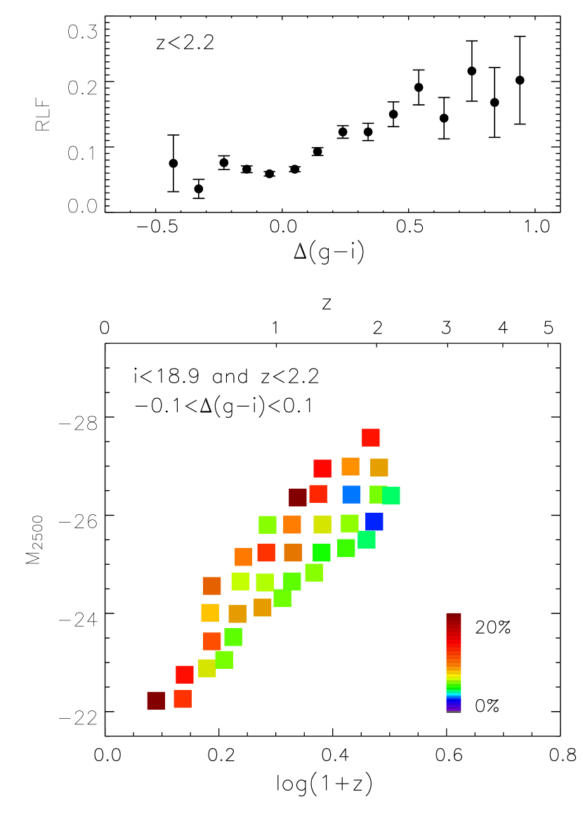
Figure 8: Upper panel: RLF as a function of $\Delta(g-i)$. The RLF rises with increasing $\Delta(g-i)$ at $z<2.2$. Lower panel: RLF as a function of $z$ and $M_{2500}$ in a small color range of $-0.1<\Delta(g-i)<0.1$.

When examining the dependence of the RLF on $M_{2500}$ and $z$, we note that contours of constant RLF in Figure 2 roughly coincide with contours of constant apparent magnitude. This is illustrated in Figure 7(a), which shows that for different redshift bins, the relation between the RLF and apparent i magnitude is independent of redshift at $i>17.5$. The RLF does decrease with redshift at $i<17.5$, although with large error bars. This “conspiracy” of strong dependence of the RLF on apparent magnitude raises the concern that our results have been affected by flux-dependent selection effects. In this paper we are considering the RLF for optically-selected quasars, and the SDSS color selection is highly complete at $z<2.2$ (Richards et al., 2006), so optical selection effects are not likely to seriously affect the RLF determination. However, the SDSS quasar selection becomes increasingly incomplete for objects with very red intrinsic colors ($\alpha<-1.5$, Fan et al., 2001; Richards et al., 2002), especially at high redshift. White et al. (2006) found a strong correlation between radio loudness and optical color using the SDSS sample. We reproduce this dependence in the upper panel of Figure 8. The RLF rises with increasing $\Delta(g-i)$, which is the difference between the observed $g-i$ and the median $g-i$ color of quasars at that redshift, following Hopkins et al. (2004). To examine whether this RLF-color dependence affects the relation in Equation 3, we divide the quasar sample into several $\Delta(g-i)$ bins, and calculate the RLF as a function of $M_{2500}$ and $z$ for each bin of intrinsic quasar colors. We find that although the average RLF increases toward redder continuum, the RLF is still a strong function of $M_{2500}$ and $z$ within each bin, similar to the relation shown in Equation 3. The lower panel of Figure 8 gives an example for the bin of $-0.1<\Delta(g-i)<0.1$. Note that more than 80% of the quasars in the sample lie in the range of $-0.3<\Delta(g-i)<0.2$, within which the RLF-color relation is relatively flat. Therefore, although we can not determine accurately the RLF evolution for the reddest few percent of quasars where SDSS is incomplete, the strong correlation between the RLF and both redshift and luminosity is not strongly affected by the RLF-color relation over the color range in which the SDSS selection is essentially complete.

In order to examine radio selection effects, we performed the following tests.

1. Did we miss FR1 quasars due to the 5$\arcsec$ radio catalog matching? We used a 10$\arcsec$ matching instead, and found that the number of FR1 quasars increases by only 3.7%. We also found that these additional sources increase the RLF by similar factors at both high and low redshift and both high and low luminosity, and thus have little effect on $b_{z}$ or $b_{M}$.

2. Did we measure the radio fluxes of FR2 quasars correctly? We compared FIRST with the NRAO VLA Sky Survey (NVSS; Condon et al., 1998), which has a resolution of 45$\arcsec$. The FIRST and NVSS fluxes of most FR2 quasars are in good agreement. FIRST has a resolution of 5$\arcsec$ and may overresolve radio sources larger than about 10$\arcsec$. These sources are rare and very bright in radio (usually $>50$ mJy), well above the radio-loud division in our analysis.

3. Were there quasars detected by NVSS but not by FIRST? We matched our sample to the NVSS catalog within 15$\arcsec$. We found that about 6% of the matched quasars were not detected by FIRST, and 80% of these additional sources are FR1 sources with offsets more than 5$\arcsec$ from the SDSS positions. They increase the RLF by similar factors at both high and low redshift and both high and low luminosity, and thus do not significantly change the trend in the RLF.

4. How did the incompleteness of FIRST at the detection limit affect our results? In Section 3 we use 1.1 mJy as the FIRST detection limit, and we correct for the incompleteness caused by the resolution effect. Here we set two tests to examine the incompleteness near the FIRST limit. In Test 6 we use a limit of 1.5 mJy (the corresponding $i\sim 18.6$) to determine the RLF for $R>10$; while in Test 7 we use a limit of 3 mJy (the corresponding $i\sim 18.9$) to calculate the RLF for $R>30$. Note that the FIRST completeness measured from the completeness curve in Figure 1 is 75% at 1.5 mJy and 95% at 3 mJy. The results of the tests are given in Table 1, and they show the similar trend of the RLF on redshift and optical luminosity as we obtained above.

Therefore, based on these tests we conclude that the strong dependence of the RLF on $M_{2500}$ and $z$ is highly likely to be physical, and the radio incompleteness and selection effects we have considered are not responsible for the dependence, though we cannot rule out other unexplored selection effects.

5 Discussion

Most of the previous studies of the RLF are based on samples of tens to hundreds of quasars. Considering that the RLF is only $\sim 10$% on average, these samples are not large enough to study the two-dimensional distribution of the RLF on $M_{2500}$ and $z$. This makes it difficult to uncover the relation of Equation 3 using only the marginal distribution of the RLF. We calculate the marginal RLF as a function of $M_{2500}$ and $z$ for our sample, which is shown in Figures 7(b) and 7(c). One can see the marginal RLF is roughly independent of both $M_{2500}$ and $z$, because the dependence on $M_{2500}$ and $z$ roughly cancel out due to the $M_{2500}$–$z$ degeneracy. This result is in quantitative agreement with the marginal RLF derived by Ivezić et al. (2002).

It has been suggested that high-redshift quasars show little difference in their rest-frame UV/optical and X-ray properties from those of low-redshift quasars. Their emission-line strengths and UV continuum shapes are very similar to those of low-redshift quasars (e.g. Barth et al., 2003; Pentericci et al., 2003; Fan et al., 2004), the emission line ratios indicate solar or supersolar metallicity in emission-line regions as found in low-redshift quasars (e.g. Hamann & Ferland, 1999; Dietrich et al., 2003; Maiolino et al., 2003), and the optical-to-X-ray flux ratios and X-ray continuum shapes show little evolution with redshift (e.g. Strateva et al., 2005; Steffen et al., 2006; Shemmer et al., 2006). These measurements suggest that most quasar properties are not sensitive to the cosmic age. However, Figure 2 shows that the RLF evolves strongly with redshift, thus the evolution of the RLF places important constraints on models of quasar evolution and the radio emission mechanism.

Equation 3 implies a strong correlation between the RLF and optical luminosity. Using a large sample of low-redshift ($0.03<z<0.3$) AGNs, Best et al. (2005) find that radio-loud AGNs tend to reside in old, massive galaxies, and that the fraction of radio-loud AGNs is a strong function of stellar mass or central black hole mass (e.g., the fraction increases from zero at a stellar mass of $10^{10}$M_☉ to 30% at a stellar mass of $5\times 10^{11}$M_☉). Assuming that optical luminosity is roughly proportional to black hole mass (Peterson et al., 2004), their radio-loud fraction of AGNs is also a strong function of optical luminosity. This is in qualitative agreement with Equation 3, although our quasars are more luminous than their low-redshift AGNs.

Equation 3 also shows that the RLF is a strong function of redshift. By stacking FIRST images of SDSS-selected quasars, White et al. (2006) recently found that the median $R$ is a declining function with optical luminosity. After correcting for this effect, they claimed that the median $R$ is independent on redshift, which seems inconsistent with our result that the RLF is a strong negative function of redshift. However, the median $R$ and the RLF are not identical. The median $R$ is determined by the majority of quasars with low $R$ values (i.e. radio-quiet quasars); while the RLF is the fraction of quasars exceeding a threshold in $R$, and therefore corresponds to the behavior of the small fraction of quasars with high $R$ values (i.e. radio-loud quasars). There are two natural ways to interpret the evolution of the RLF with redshift (e.g. Peacock, Miller, & Longair, 1986): (1) This may be due to the cosmological evolution of quasar radio properties, such as $R$ and $L_{r}$. For instance, a decreasing $R$ results in a decreasing RLF for increasing redshift. (2) This could be simply caused by the density evolution of different populations of quasars (e.g. radio-loud and radio-quiet quasars). The results of White et al. (2006) may have ruled out the first explanation and leave the second one: the different density evolution behaviors for the two classes of quasars. For instance, there are more radio-loud quasars at low redshift, but the fraction of radio-loud quasars is small, so they do not change the median $R$, which is still dominated by radio-quiet quasars. This claim is based on stacked FIRST images. To distinguish between the two explanations, one needs to determine the radio luminosity function of quasars in different redshift ranges, including the radio-quiet population, going to radio fluxes much fainter than those probed by FIRST. Deep surveys such as the Cosmic Evolution Survey (Schinnerer et al., 2004) that cover a wide redshift range and reach low luminosity in both optical and radio wavelengths are needed to interpret the evolution of the RLF.

6 Summary

In this paper we use a sample of more than 30,000 optically-selected quasars from SDSS to determine the RLF of quasars as a function of redshift and optical luminosity. The sample covers a large range of redshift and luminosity. We study the RLF using different criteria to define radio-loud quasars. After breaking the degeneracy between redshift and luminosity, we find that the RLF is a strong function of both redshift and optical luminosity: the RLF decreases rapidly with increasing redshift and decreasing luminosity. The relation can be described by a simple model, given by Equation 3. We have done a series of tests to examine the impact of flux-related selection effects, and find that the dependence of the RLF on redshift and luminosity is highly likely to be physical.

The RLF is one of a few quasar properties that strongly evolve with redshift, so the evolution of the RLF places important constraints on models of quasar evolution and the radio emission mechanism. By comparing our results with the behavior of the median $R$ derived from stacked FIRST images, we find that the evolution of the RLF with redshift could be explained by the different density evolution for radio-loud and radio-quiet quasars. Substantially deeper wide-angle radio surveys which obtain fluxes for the radio-quiet population are needed to fully understand the physical nature of this evolution.

Table 1: Results of fits to Equation 3

Sample	$\chi^{2}$	DoF	$b_{0}$	$b_{z}$	$b_{M}$	Cov($b_{z}$,$b_{M}$)
$R>10$	52.8	47	$-0.132\pm 0.116$	$-2.052\pm 0.261$	$-0.183\pm 0.025$	0.0059
$R>30$	50.7	45	$-0.218\pm 0.110$	$-2.096\pm 0.240$	$-0.203\pm 0.023$	0.0050
$\log L_{r}>32$	30.3	35	$-0.053\pm 0.122$	$-2.214\pm 0.277$	$-0.307\pm 0.024$	0.0055
$\log L_{r}>32.5$	45.2	41	$-0.216\pm 0.118$	$-2.088\pm 0.260$	$-0.333\pm 0.025$	0.0055
Test 1 ($R>10$)	62.1	48	$-0.328\pm 0.115$	$-1.639\pm 0.259$	$-0.141\pm 0.024$	0.0058
Test 2 ($R>10$)	64.4	46	$-0.292\pm 0.116$	$-1.693\pm 0.259$	$-0.165\pm 0.024$	0.0058
Test 3 ($R>10$)	57.0	46	$-0.308\pm 0.114$	$-1.722\pm 0.261$	$-0.123\pm 0.024$	0.0058
Test 4 ($R>10$)	53.6	46	$-0.142\pm 0.120$	$-2.115\pm 0.268$	$-0.194\pm 0.025$	0.0063
Test 5 ($R>10$)	78.9	46	$0.120\pm 0.102$	$-2.924\pm 0.258$	$-0.254\pm 0.022$	0.0054
Test 6 ($R>10$)	51.9	41	$-0.104\pm 0.148$	$-2.137\pm 0.347$	$-0.185\pm 0.032$	0.0106
Test 7 ($R>30$)	49.2	45	$-0.213\pm 0.128$	$-2.115\pm 0.286$	$-0.202\pm 0.027$	0.0071

Figure 1: The FIRST completeness as a function of integrated flux density (provided by R. L. White, private communication). The completeness is computed using the observed size distribution of SDSS quasars and rms values of integrated flux densities from the FIRST survey.

Figure 3: RLF in three small redshift ranges and three small magnitude ranges. Dotted lines are the best model fits.

Figure 4: $1\sigma$, $2\sigma$ and $3\sigma$ confidence regions for $b_{z}$ vs. $b_{M}$.

Figure 5: The $R$-based RLF as a function of $z$ and $M_{2500}$. The upper panels show the RLF as a function of redshift after correcting for the luminosity dependence and the lower panels show the RLF as a function of luminosity after correcting for the redshift dependence. Filled circles are RLFs calculated from individual $M_{2500}$–$z$ grids and dashed lines are the best model fits. Poisson errors are also given in the figure.

Figure 6: The $L_{r}$-based RLF as a function of $z$ and $M_{2500}$. The upper panels show the RLF as a function of redshift after correcting for the luminosity dependence and the lower panels show the RLF as a function of luminosity after correcting for the redshift dependence. Filled circles are RLFs calculated from individual $M_{2500}$–$z$ grids and dashed lines are the best model fits. Poisson errors are also given in the figure.

References

- Abazajian et al. (2005) Abazajian, K., et al. 2005, AJ, 129, 1755
- Baum et al. (1995) Baum, S. A., Zirbel, E. L., & O’Dea, C. P. 1995, ApJ, 451, 88
- Barth et al. (2003) Barth, A. J., Martini, P., Nelson, C. H., & Ho, L. C. 2003, ApJ, 594, L95
- Barthel (1989) Barthel, P. D. 1989, ApJ, 336, 606
- Becker, White, & Helfand (1995) Becker, R. H., White, R. L., & Helfand, D. J. 1995, ApJ, 450, 559
- Best et al. (2005) Best, P. N., Kauffmann, G., Heckman, T. M., Brinchmann, J., Charlot, S., Ivezić, Ž., & White, S. D. M. 2005, MNRAS, 362, 25
- Bischof & Becker (1997) Bischof, O. B., & Becker, R. H., AJ, 113, 2000
- Cirasuolo et al. (2003) Cirasuolo, M., Magliocchetti, M., Celotti, A., & Danese, L. 2003, MNRAS, 341, 993
- Condon et al. (1998) Condon, J. J., Cotton, W. D., Greisen, E. W., Yin, Q. F., Perley, R. A., Taylor, G. B., & Broderick, J. J. 1998, AJ, 115, 1693
- de Vries, Becker, & White (2006) de Vries, W. H., Becker, R. H., & White, R. L. 2006, AJ, 131, 666
- Dietrich et al. (2003) Dietrich, M., Hamann, F., Appenzeller, I., & Vestergaard, M. 2003, ApJ, 596, 817
- Fan et al. (2001) Fan, X., et al. 2001, AJ, 121, 31
- Fan et al. (2004) Fan, X., et al. 2004, AJ, 128, 515
- Fukugita et al. (1996) Fukugita, M., Ichikawa, T., Gunn, J. E., Doi, M., Shimasaku, K., & Schneider, D. P. 1996, AJ, 111, 1748
- Goldschmidt et al. (1999) Goldschmidt, P., Kukula, M. J., Miller, L., & Dunlop, J. S. 1999, ApJ, 511, 612
- Gunn et al. (1998) Gunn, J. E., et al. 1998, AJ, 116, 3040
- Gunn et al. (2006) Gunn, J. E., et al. 2006, AJ, 131, 2332
- Hamann & Ferland (1999) Hamann, F., & Ferland, G. 1999, ARA&A, 37, 487
- Hooper et al. (1995) Hooper, E. J., Impey, C. D., Foltz, C. B., & Hewett, P. C. 1995, ApJ, 445, 62
- Hopkins et al. (2004) Hopkins, P. F., et al. 2004, AJ, 128, 1112
- Ivezić et al. (2002) Ivezić, Ž., et al. 2002, AJ, 124, 2364
- Ivezić et al. (2004a) Ivezić, Ž., et al. 2004, in AGN Physics with the Sloan Digital Sky Survey, eds. G. T. Richards and P. B. Hall, ASP Conference Series, Vol. 311, p. 347 (also astro-ph/0310569)
- Ivezić et al. (2004b) Ivezić, Ž., et al. 2004, in Multiwavelength AGN Surveys, eds. R. Mujica and R. Maiolino, World Scientific Publishing Company, Singapore, p. 53 (also astro-ph/0403314)
- Jiang et al. (2006) Jiang, L., et al. 2006, AJ, 131, 2788
- Kellermann et al. (1989) Kellermann, K. I., Sramek, R., Schmidt, M., Shaffer, D. B., & Green, R. 1989, AJ, 98, 1195
- Lacy et al. (2001) Lacy, M., Laurent-Muehleisen, S. A., Ridgway, S. E., Becker, R. H., & White, R. L. 2001, ApJ, 551, L17
- Laor (2000) Laor, A. 2000, ApJ, 543, L111
- Maiolino et al. (2003) Maiolino, R., Juarez, Y., Mujica, R., Nagar, N. M., & Oliva, E. 2003, ApJ, 596, L155
- Matthews & Sandage (1963) Matthews, T. A., & Sandage, A. R. 1963, ApJ, 138, 30
- McLure & Jarvis (2004) McLure, R. J., & Jarvis, M. J. 2004, MNRAS, 353, L45
- Miller, Peacock, & Mead (1990) Miller, L., Peacock, J. A., & Mead, A. R. G. 1990, MNRAS, 244, 207
- Padovani (1993) Padovani, P. 1993, MNRAS, 263, 461
- Peacock, Miller, & Longair (1986) Peacock, J. A., Miller, L., & Longair M. S. 1986, MNRAS, 218, 265
- Pentericci et al. (2003) Pentericci, L., et al. 2003, A&A, 410, 75
- Peterson et al. (2004) Peterson, B. M., et al. 2004, ApJ, 613, 682
- Richards et al. (2002) Richards, G. T., et al. 2002, AJ, 123, 2945
- Richards et al. (2006) Richards, G. T., et al. 2006, AJ, 131, 2766
- Sandage (1965) Sandage, A. 1965, ApJ, 141, 1560
- Schlegel, Finkbeiner, & Davis (1998) Schlegel, D. J., Finkbeiner, D. P., & Davis, M. 1998, ApJ, 500, 525
- Schinnerer et al. (2004) Schinnerer, E., et al. 2004, AJ, 128, 1974
- Schmidt (1963) Schmidt, M. 1963, Nature, 197, 1040
- Schneider et al. (1992) Schneider, D. P., van Gorkom, J. H., Schmidt, M., & Gunn, J. E. 1992, AJ, 103, 1451
- Schneider et al. (2005) Schneider, D. P., et al. 2005, AJ, 130, 367
- Shemmer et al. (2006) Shemmer, O., et al. 2006, ApJ, 644, 86
- Spergel et al. (2006) Spergel, D. N., et al. 2006, submitted to ApJ (astro-ph/0603449)
- Steffen et al. (2006) Steffen, A. T., et al. 2006, AJ, 131, 2826
- Stern et al. (2000) Stern, D., Djorgovski, S. G., Perley, R. A., de Carvalho, R. R., & Wall, J. V. 2000, AJ, 119, 1526
- Stocke et al. (1992) Stocke, J. T., Morris, S. L., Weymann, R. J., & Foltz, C. B. 1992, ApJ, 396, 487
- Strateva et al. (2005) Strateva, I. V., Brandt, W. N., Schneider, D. P., Vanden Berk, D. G., & Vignali, C. 2005, AJ, 130, 387
- Urry & Padovani (1995) Urry, C. M., & Padovani P. 1995, PASP, 107, 803
- Vanden Berk et al. (2001) Vanden Berk, D. E., et al. 2001, AJ, 122, 549
- Visnovsky et al. (1992) Visnovsky, K. L., Impey, C. D., Foltz, C. B., Hewett, P. C., Weymann, R. J., & Morris, S. L. 1992, ApJ, 391, 560
- White et al. (1997) White, R. L., Becker, R. H., Helfand, D. J., & Gregg, M. D. 1997, ApJ, 475, 479
- White et al. (2006) White, R. L., Helfand, D. J., Becker, R. H., Glikman, E., & de Vries, W. 2006, ApJ, in press (astro-ph/0607335)
- York et al. (2000) York, D. G., et al. 2000, AJ, 120, 1579