Plausible fluorescent Ly$\alpha$ emitters around the $z=3.1$ QSO0420-388

Abstract

We report the results of a survey for fluorescent Ly$\alpha$ emission carried out in the field surrounding the $z=3.1$ quasar QSO0420-388 using the Focal Reducer/Low Disperion Spectrograph 2 (FORS2) instrument on the Very Large Telescope (VLT). We first review the properties expected for fluorescent Ly$\alpha$ emitters, compared with those of other non-fluorescent Ly$\alpha$ emitters. Our observational search detected 13 Ly$\alpha$ sources sparsely sampling a volume of $\sim 14000$ comoving Mpc³ around the quasar. The properties of these in terms of (1) the line equivalent width, (2) the line profile and (3) the value of the surface brightness related to the distance from the quasar, all suggest that several of these may be plausibly fluorescent. Moreover, their number is in good agreement with the expectation from theoretical models. One of the best candidates for fluorescence is sufficiently far behind QSO0420-388 that it would imply that the quasar has been active for (at least) $\sim$60 Myr. Further studies on such objects will give information about proto-galactic clouds and on the radiative history (and beaming) of the high-redshift quasars.

1. Introduction

The analysis of absorption systems in the spectra of high-redshift quasars has represented for several decades the only practical way to obtain information about the properties of the intergalactic medium (IGM). The Ly$\alpha$ forest gives an unique insight into the one-dimensional distribution of low density hydrogen along the quasars’ line of sight. Higher column-density features, i.e. the Lyman-limit systems (LLSs) and the damped Ly$\alpha$ systems (DLAs), correspond to denser concentrations of atomic hydrogen and, for this reason, can be associated with galaxy formation. Unfortunately the information from quasar absorption spectra is almost always one-dimensional.

An interesting alternative to absorption studies is to try to detect the IGM in emission rather than in absorption. The absorption of ionizing photons should be associated with the emission of fluorescent Ly$\alpha$ photons, as originally proposed by Hogan & Weymann (1987). Detection of the fluorescent emission would provide a three-dimensional picture of the neutral IGM and proto-galactic clouds at high redshift.

In an earlier paper (Cantalupo et al. 2005, hereafter Paper I), we constructed models of fluorescent emission in realistic hydrodynamical simulations. These simulations were normalized so as to produce the correct statistics for Lyman limit absorption systems. For clouds that are optically thick to the ionizing radiation (i.e. Lyman limit systems and above), the surface brightness (SB) of the fluorescent emission is set by the strength of the ionizing background. Unfortunately, the intensity of the UV background at $z\sim 3$ (e.g. Haardt & Madau 1996) corresponds to a maximum Ly$\alpha$ SB of $\sim 3\times 10^{-20}$$\mathrm{erg}\ \mathrm{s}^{-1}\mathrm{cm}^{-2}\mathrm{arcsec}^{-2}$ . Detecting such a low SB is very challenging with present-day instrumentation. Blind searches in the field have only produced a number of null results (Lowenthal et al. 1990; Martínez-Gonzalez et al. 1995; Bunker, Marleau & Graham 1998).

The SB of fluorescent emission will be higher if the local ionizing background is increased, e.g. for gas clouds lying close to a bright quasar. In Paper I, we examined this effect and showed that it could boost the fluorescent emission to detectable levels over a large volume, i.e. of order 30,000 comoving Mpc³ for a sufficiently bright quasar. The penalty for this boost is that the extra photo-ionization increases the total hydrogen column density that is required to reach a given neutral column density, i.e. to produce the maximum fluorescent surface brightness. This is the analogue of the proximity effect seen in quasar absorption spectra. It means that maximally fluorescent sources near to a quasar will be systems that, in the absence of the quasar, would be DLAs rather than LLS. DLAs have hydrogen column densities comparable to a sightline through the disk of present day spiral galaxies and a total gas mass similar to the mass in stars and gas within galaxies at the present epoch (Wolfe et al. 1995). For these reasons, DLAs are widely believed to be the gas reservoirs from which the present galaxies formed. However, it is still unclear if DLAs are galaxies already in place (e.g. Prochaska & Wolfe 1998) or are still in the form of protogalactic clouds (e.g. Haehnelt, Steinmetz & Rauch 1998). They typically contain very little of the molecular hydrogen usually associated with star formation (e.g. Ledoux et al. 2003, but see also Zwaan & Prochaska 2006). Moreover, metallicity measurements show a large range from 1/10 solar to a value close to that measured for the Ly$\alpha$ forest (cf. Prochaska et al. 2003 and Simcoe et al. 2004). It is likely that DLAs include systems of different origins.

In addition to studying the intergalactic medium, the detection and measurement of fluorescent Ly$\alpha$ emission from clouds at different distances and orientations from the quasar, would in principle allow the study of the history and angular distribution of the ultraviolet emission from quasars. Both questions are of considerable topical interest in the context of unified models of active galactic nuclei (see e.g. Antonucci 1993).

In this paper we describe a blind survey for fluorescent Ly$\alpha$ emission carried out around the $z\sim 3.1$ quasar QSO0420-388, one of the brightest quasars at high redshift for which the Ly$\alpha$ line lies within an existing narrow-band filter of the VLT-FORS2 instrument.

Previous searches for fluorescence around quasars have had either null results at $z\sim 2.2$ (Francis & Bland-Hawthorn 2004) or only one (or marginally two) possible detection at $z\sim 4.3$ (Francis & McDonnell 2006). In the first case, the null result is perfectly consistent with our model of fluorescent Ly$\alpha$ emission presented in Paper I. In the second case, the very close association of the system with the quasar itself makes the identification with fluorescence difficult (see section 2.5 for details). Other possible fluorescent sources have been detected serendipitously in connection with absorbing systems in quasar pairs (Fynbo et al. 1999, Adelberger et al. 2006). However, the metallicity of the systems and the presence of a substantial continuum emission probably indicate the presence of star formation within the clouds. Ly$\alpha$ emission at high redshift can of course be produced by internally ionized clouds, either from an associated young stellar population or from processes involving the gas itself (e.g. cooling). Several observations during the last decade have shown that these emitters are quite common in the high-redshift universe (for a review see Taniguchi et al. 2003) and enhanced by clustering effects around bright sources like AGNs and, in particular, radio-galaxies (e.g. Venemans et al. 2005 and references therein). In searching for fluorescence, we must thus take into account the presence of this population.

The layout of the paper is as follows. In §2 we compare the characteristics of fluorescent Ly$\alpha$ emission with those of other sources of Ly$\alpha$ emission at high redshift, in order to determine which properties can best be used to recognize fluorescent emission. Although fluorescent sources should have characteristic equivalent widths (extremely high), SB and spectral profiles, none of these provide a unique diagnostic. We conclude this section by reviewing recent claims in the literature for detected fluorescence. In §3 we describe our own new observations and the data reduction. We then isolate a set of Ly$\alpha$ emitting candidates around the target quasar. In §4, we discuss in detail the properties of the individual sources in the context of the expected fluorescent characteristics, and compare their number density with both our own models for fluorescence (Paper I) and those of other non-fluorescent Ly$\alpha$ sources. We conclude that it is likely, but not certain, that some of the detected sources that we have detected are indeed fluorescent. In §5 we summarize the paper.

2. Recognition of fluorescent emission

Besides fluorescent emission, Ly$\alpha$ can be produced by several kinds of internal sources, e.g. photo-ionization from a young stellar population or active nucleus (LAE, Ly$\alpha$ emitter [galaxies]), or from cooling of shock-heated gas. Many observations during the last decade have shown that Ly$\alpha$ emitters are quite common in the high-redshift universe (e.g. Cowie & Hu 1998; Pascarelle, Windhorst & Kell 1998; Fynbo et al. 2003) and enhanced by clustering effects around objects like AGNs and, in particular, radio-galaxies (e.g. Le Fevre et al.1996; Pascarelle et al. 1996; Venemans et al. 2005) which likely reside in high density regions of the Universe.

In this section, we review the characteristic properties that in principle could identify a source as fluorescent: i) the equivalent width (EW), ii) the emission profile, iii) the surface brightness (SB), and iv) the number density of emitters. We will take advantage of the model recently presented in Paper I, in which a combination of a high-resolution hydrodynamic simulation and two radiative transfer schemes was used to predict the properties, spectra and number density of fluorescent Ly$\alpha$ emitters at $z\sim 3$.

2.1. Equivalent Widths

In the fluorescent case, the Ly$\alpha$ emission originates from pure gaseous clouds externally photo-ionized. Therefore, any continuum emission comes only from recombination processes: mainly two-photon continuum and free-bound recombinations. However, given the low value of the emission coefficient corresponding to these processes, the continuum level around the Ly$\alpha$ wavelength is very faint, resulting in an extremely high EW. The case of Ly$\alpha$ emission originating from cooling shock-heated gas will be similar.

If the Ly$\alpha$ emission results from photo-ionization by embedded young stars, we expect a significant contribution to the UV continuum emission from the stellar population. In this case, the Ly$\alpha$ EW depends on the age, initial mass function (IMF), metallicity and dust content of the star-formation burst. Synthesis population models (see e.g. Schaerer 2003 and references therein) show that high EWs can be produced for very young bursts in metal-poor and dust-free galaxies. Upper limits for very metal-poor models ($0<Z<10^{-7}$) range from EW$\sim 800\mathrm{\AA}$ (for a very young population with an age of 2 Myr) to EW$\sim 200\mathrm{\AA}$ (for a 10 Myr old star-formation burst). Synthesis models of star-forming galaxies with moderate ages ($>10$ Myr) and with metallicity (and IMF) closer to the normally observed values have EW in the range $50-200$ $\mathrm{\AA}$ (Charlot & Fall 1993). Surveys of Ly$\alpha$ emitters at $z\sim 3$ usually show a distribution of EW in the range from $15-100\mathrm{\AA}$, with a few objects extending to higher values (up to 200-300$\mathrm{\AA}$). High-EW objects can also be associated with AGN activity.

2.2. Emission line profiles

The properties of the Ly$\alpha$ line have been widely studied analytically under certain approximations (e.g. Neufeld 1990 and references therein). In particular, for an extremely opaque and plane-parallel medium, it is possible to demonstrate that the emerging profile consists of two symmetric peaks separated by a velocity shift of $\Delta v\sim 2(\ln\tau_{\mathrm{Ly}\alpha})^{1/2}\sqrt{2}\sigma_{\mathrm{th}}$ (where $\tau_{\mathrm{Ly}\alpha}$ and $\sigma_{\mathrm{th}}$ are, respectively, the central-line optical depth of Ly$\alpha$ photons and the thermal velocity dispersion of the medium).

Since fluorescent photons originate from externally ionized clouds, their typical $\tau_{\mathrm{Ly}\alpha}$ should correspond to $\tau_{\mathrm{Ly}\alpha}\sim 2\times 10^{4}$ (assuming a temperature of $T=2\times 10^{4}$ K). Therefore, in the above approximations, fluorescent emission should be characterized by two symmetric peaks separated by $\Delta v\sim 8.9\sigma_{\mathrm{th}}$.

However, detailed simulations of fluorescent emission in more realistic situations show that the inclusion of velocity fields inside and around the clouds influences the emerging line profile. In most cases, the symmetry of the double-humped profile is lost and one of the two peaks is severely suppressed (see Fig. 7 in Paper I; notice that the x-scale of that figure is erroneously multiplied by a factor of 4). Furthermore, if the gas consists of several small clumps, a turbulent velocity term should be added to the thermal velocity dispersion, increasing the separation of the peaks. On the other hand, if the turbulent velocity of the emitting region is large compared with that of the intervening layers, the symmetry of the line profile may be restored.

While the double peaked nature of fluorescent emission can be modified, the single Ly$\alpha$ lines generated by internal photo-ionization at low optical depth can be partially absorbed by infalling or expanding gas. As a result, the emergent profile can again consist of multiple components.

We conclude that these practicalities mean that the analysis of the emission line profile alone cannot provide a watertight signature of fluorescence.

Table 1 Summary of the observations and setups.

Setup name	Date	Mode	Filter	Mask rotation	Combined seeing	Exposure time
S1	Nov. 29	MXU	OIII/3000+51	0o	1”.0	25 200 s
S2	Nov. 30 and Dec. 1	MXU	OIII/3000+51	90o	1”.0	34 200 s
IMA	Dec. 1	Imaging	Bessel V	-	1”.0	7 200 s
S3	Dec. 2	MXU	OIII+50	0o	0”.7	23 400 s

2.3. Surface Brightness

With a simplified slab geometry (e.g. Hogan & Weymann 1987, Gould & Weinberg 1996) of a semi-infinite and static medium, fluorescent (self-shielded) clouds should act like “mirrors”: illuminated by an external source they return the incident ionizing photons in the form of Ly$\alpha$ line emission with an efficiency of $\sim 65\%$. In this case, the Ly$\alpha$ SB is uniform and its value is easily predicted once the impinging ionizing flux is known, and vice-versa.

In the case of a locally enhanced ionizing flux, e.g. from a nearby quasar, the fluorescent SB would be expected in this simplified geometry to be higher. We introduce a “boost factor” $b$, which is defined as the increase in the predicted SB relative to that induced by the UV background at $z\sim 3$ (${\mathrm{SB}}_{\mathrm{bg}}=3.67\times 10^{-20}$$\mathrm{erg}\ \mathrm{s}^{-1}\mathrm{cm}^{-2}\mathrm{arcsec}^{-2}$), i.e. SB$=(1+b)$SB_bg. The value of $b$ corresponds to:

$$b=15.2\,\frac{L_{\rm LL}}{10^{30}\,\mathrm{erg}\,\mathrm{s}^{-1}\,\mathrm{Hz}^{-1}}\,\frac{0.7}{\alpha}\,\left(\frac{r}{\mathrm{1\,Mpc}}\right)^{-2}$$ (1)

at a physical distance $r$ from a quasar with monochromatic luminosity $L_{\nu}=L_{\rm LL}(\nu/\nu_{\rm LL})^{-\alpha}$ (see figs.6,9 and section 3.3 in Paper I for further details).

When velocity fields and a more realistic gas distribution are taken into account, it is found (Paper I) that the SB may be reduced. In particular, for anisotropic illumination (i.e. fluorescence induced by a quasar), the expected SB in the direction of the incoming flux can be much lower than expected in the slab approximation. The importance of this effect, which we called the “geometric effect”, depends on the relative size of the shielding-layer with respect to the cloud radius, and therefore on the gas density profile and the intensity of the impinging radiation. In Paper I, we found that the fluorescent SB from self-shielded clouds is still predictable in good approximation from the empirical relation:

$$\mathrm{SB}=(0.74+0.50\,b^{0.89})\mathrm{SB}_{\mathrm{bg}}\,$$ (2)

where $b$ represents the ideal “boost factor” described above.

The SB predicted in this way represents a fundamental upper-limit constraint: emitters with higher SB must receive a ionizing contribution from other sources and, therefore, are with high probability internally ionized clouds. However, several uncertainties remain to be taken into account. In particular, the exact distance from the quasar may be uncertain due to peculiar motions (and uncertainty in the precise systemic redshift of the quasar). Anisotropy or time-variability in the quasar emission will also modify the SB. In fact this latter effect offers the possibility, if other indicators indicate a fluorescent origin of the emission, that their SBes can be used to study the angular distribution and temporal history of the quasar UV emission.

2.4. The number density of emitters

The covering factor of fluorescent sources on the sky within a volume is directly related to the number density of optically thick absorbers seen in quasar spectra. This fact was used in Paper I to normalise our simulations. Two complications enter in the present case. First, the regions around quasars are likely to have higher than average density. Second, the enhanced ionizing radiation will produce a higher photo-ionization in a given cloud, reducing the column density of neutral Hydrogen. The high surface brightness fluorescence will still come from systems which would be seen as LLS if there was a background quasar, but these are systems that would have been seen as DLA if the extra ionizing radiation had not been present. The fluorescence near to a quasar is thus closely linked to the “proximity effect” (e.g. Bajtlik, Duncan & Ostriker 1988). Since statistics of LLS near QSOs are not constrained, we must rely on theoretical models to determine their covering factor.

The procedure to calculate the expected number of fluorescent emitters around a quasar, outlined in section 3.4 in Paper I, consists of three steps: i) convert the SB sensitivity limit of the survey (SB_lim) into a minimum boost factor $b_{\mathrm{min}}$ inverting Eq.(2), ii) use $b=b_{\mathrm{min}}$ in Figure 11 of Paper I to determine the physical number density of fluorescent sources with SB$\geq$SB_lim; iii) given the values of $L_{\mathrm{LL}}$, $\alpha$ for the selected quasar, invert Eq. 1 using $b=b_{\mathrm{min}}$ to find the maximum distance ($r_{\mathrm{max}}$), and thus the volume, where the fluorescent SB$\geq$SB_lim. As an example, a sensitivity of SB${}_{\rm lim}\sim 10^{-18}$$\mathrm{erg}\ \mathrm{s}^{-1}\mathrm{cm}^{-2}\mathrm{arcsec}^{-2}$ corresponds to a fluorescent (physical) number density of $\mathrm{dN}/\mathrm{dV}\sim 0.3\pm 0.1$ Mpc^-3 (for sources with area $A\simeq 4$ arcsec²), neglecting any density enhancement around the quasar.

This may be compared with the number density of other Ly$\alpha$ sources around $z\sim 3$ quasars. Recent surveys indicate that the number of Ly$\alpha$ emitters around radio-galaxies at that redshift can be enhanced by a factor $\sim 3$ with respect to the field. In particular, Venemans et al. (2005; hereafter V05) found an emitter number density of $0.26\pm 0.04$ Mpc^-3 around the $z\sim 3.13$ radio-galaxy MRC0316-257, in a survey with sensitivity of the order of SB${}_{\rm lim}\sim 10^{-18}$$\mathrm{erg}\ \mathrm{s}^{-1}\mathrm{cm}^{-2}\mathrm{arcsec}^{-2}$ . In the view of the AGN unified model (see e.g. Antonucci 1993), the environment of radio-loud quasars should be similar to that of radio-galaxies. Moreover, we do not expect a significant contribution from fluorescent sources to the number density found by V05, given the shape of their survey and the direction of the (probable) UV emission-cone from MRC0316-257.

2.5. Fluorescent candidates in the literature

In this section, we briefly describe previous surveys for fluorescent emission and review the results of these in the light of our discussion above. Given the difficulties in the detection of fluorescence induced by the UV-background alone, previous surveys have centered around quasars, as in our case.

Francis & Bland-Hawtorn (2004) reported an attempt to find fluorescence around a quasar at redshift $\sim 2.17$ basing their expectations on the simplified analytical models (Gould & Weinberg 1996). In particular, they were expecting to find at least 6 fluorescent emitters within their sampled region of 1 Mpc around the quasar, but they saw none. However, this result is perfectly consistent with the expectation of our more realistic model of fluorescent emission (see section 3.5 in Paper I for details).

Adelberger et al. (2006) reported the serendipitous discovery of a possible fluorescent emitter associated with a DLA at redshift $\sim 2.8$. In particular they found the emitter in the spectrum of a Lyman-break object located 49” from a much brighter quasar. The object consists of two peaks with separation $\Delta V\sim 500$ km s^-1 and its SB seems to be compatible with the fluorescence induced by the quasar, even though the required boost factor is extremely high ($b\sim 2000$, in the ideal case of a slab). However, the object is clearly detected in their $G$ and $R$ images (with an observed magnitude $G_{\rm AB}=26.8\pm 0.2$) resulting in a rest-frame equivalent width EW${}_{0}=72\pm 20\mathrm{\AA}$. Therefore, this candidate is more plausibly an internally ionized source. A similar detection, associated with a lower redshift DLA system ($z\sim 1.9$) in the spectrum of a close quasar-pair, was reported by Fynbo et al. (1999). In this case a continuum counterpart is not clearly detected, although the subtraction of the PSF of the bright quasars makes this difficult. However, the extreme proximity of the quasar responsible of the possible fluorescent emission ($\sim 20$kpc), indicates a plausible physical connection between the two objects.

Finally, Francis & McDonnell (2006) claimed the detection of a fluorescent object located just 0.8” from a quasar at $z=4.28$. Their object is spectrally and spatially unresolved and the flux is poorly constrained because of the proximity of the quasar. There is a lower limit for the equivalent width of EW${}_{0}>19\mathrm{\AA}$. Given the vicinity of the quasar ($\sim 5-50$ physical kpc) and the uncertainties in the flux and size measurement, comparison with the theoretical SB is hard, although they note that the predicted luminosity is $\sim 400$ times greater than observed, if the object is fluorescent. The sampled area around the quasar is very small ($5^{\prime\prime}\times 7^{\prime\prime}$ in projection) because of the Integral Field Spectrometer used, making any statistical comparison difficult.

3. Observations and data analysis

In this section we describe our own survey for fluorescent emission around QSO0420-388, including the data reduction and the selection of the Ly$\alpha$ candidates.

3.1. VLT spectroscopy and imaging

Observations were taken during four visitor-mode nights on the VLT 8.2 m telescope Antu on November 28 - December 1, 2005. The FORS2 spectrograph was used in multi-object spectroscopy mode (MXU) at standard resolution ($0.25^{\prime}\times 0.25^{\prime}\ \mathrm{arcsec^{2}\ pixel^{-1}}$) to build a “multi-slit plus filter” (Crampton & Lilly 1999) configuration centered on the $z=3.1$ QSO [HB89]0420-388.

For all the observations, we used the 1400V grism giving a dispersion of 0.61 $\mathrm{\AA}$ pixel^-1, in combination with the narrow band filters OIII+50 and OIII/3000+51. The resolution (R=2100, corresponding to $\sim 150\mathrm{km}\mathrm{s^{-1}}$) is large enough to resolve the doublet [OII]$\lambda\lambda 3726,3729$, which helps to distinguish a Ly$\alpha$ emission from low redshift contaminants. The use of the narrow band filters allowed us to put 14 slits (each 6.8’ long and 2” wide) parallel to each other and separated by 25” without a significant overlapping of the spectra on the CCD. The total area covered by the slits in the mask corresponds to 3.17 arcmin². The same mask was used for all the observations. but with two different filters and two different spatial orientations: i) slits parallel to North-South direction, ii) slits parallel to East-West direction.

The use of two different narrow band filters and two mask orientations was chosen in order to increase the sampled volume in redshift and projected space. For our setup, the central wavelength of the filters OIII+50 and OIII/3000+51 is, respectively 5001$\mathrm{\AA}$ and 5045$\mathrm{\AA}$ with a FWHM of 57$\mathrm{\AA}$ and 59$\mathrm{\AA}$, corresponding to a total redshift range $z=3.089-3.173$ for Ly$\alpha$. Filter OIII/3000+51 was used for both the mask orientations (0^o and 90^o rotations) and filter OIII+50 for just one orientation (0^o rotation).

For each configuration, a series of several dithered exposures of 1800s each, stepped along the slit by 5 arcsec, were obtained for a combined exposure time of 7 hours (filter OIII+51 and 0^o rotation), 9.5 hours (filter OIII+50 and 0^o rotation) and 6.5 hours (filter OIII+51 and 90^o rotation). On the third night we also obtained a V-band image of the same field for a total exposure time of 2 hours. It consisted of 120 dithered exposures of 60 secs each, and it was obtained under photometric sky conditions. An overview of the observations and of the different configurations is summarized in Table 1.

3.2. Data reduction

The spectroscopic and photometric data were reduced using standard packages (IRAF - Image Reduction and Analysis) and additional IDL routines written by the authors.

The data reduction consisted of several steps including bias subtraction, spectral distortion correction, flat-fielding (using “sky-flats” obtained from the scientifical images themselves) and sky subtraction. The individual sky-subtracted images were then combined to obtain the three scientific images corresponding to the three different configurations (see Table 1). The combination of the images was performed with an averaged sigma clipping algorithm in order to minimize the effect of bad pixels and cosmic rays. A pixel-by-pixel noise map associated with each science image was generated from the statistics of the pixels in the multiple image combinations.

Spectro-photometric calibration was based on observations of different spectro-photometric standard stars for each night of observation. The magnitude zero-points derived from several standard stars were consistent with each other within 0.02 magnitudes. A small Galactic extinction correction of $A_{\lambda}(V)=0.079$ mag (Schlegel et al. 1998) was applied.

The result of the data reduction was three final “spectroscopic” multi-slit images (S1, S2 and S3; corresponding to the different configurations of mask orientation and filters summarized in Table 1) plus the V-band image (IMA) of the same field. The ensuing steps included: i) the detection of line emission in S1, S2 and S3; ii) the identification of possible continuum counterparts of the line emission in the V-band image; iii) the selection of probable Ly$\alpha$ emission with a criterion based on the rest-frame equivalent width of the line.

3.3. Line emission detection

The detection of line emission candidates was performed with the help of the software package SExtractor (Bertin & Arnouts 1996). In order to make the detection process more efficient, we first removed from each image the regions corresponding to the brightest continuum spectra (typically stars and local bright galaxies). Such regions were automatically identified for each slit by summing the flux over the spectral band and applying a sigma-clipping algorithm to the resulting 1-dimensional array. We removed all the regions where the integrated signal was greater than 3 times the standard deviation for that slit. The excluded regions were, respectively, $\sim 4\%$ and $\sim 9\%$ of the total image for the 0^o and 90^o rotation configurations.

The resulting images and corresponding noise-maps (obtained in the reduction process described above) were then processed by SExtractor. In order to allow the most general search, we varied the three most relevant parameters, i.e. the smoothing filter, the minimum detection threshold and the minimum detection area (i.e. the number of connected pixels). We used always standard filters (Gaussian, top hat) plus our own filters with a shape designed to increase the S/N of the double peaked emission. The minimum detection threshold and the number of connected pixel was varied, respectively, from 0.3 to 1.5, and from 3 to 30 pixels. Each combination of the three detection parameters produced a separate catalog of line emission candidates, for a total of 1344 catalogs for each dataset. We refer to these as “positive” catalogues.

We then applied exactly the same procedure on the original images after they had been multiplied by $-1$ to produce a negative image. Any emission objects detected in these “negative” catalogues must of course be spurious. We therefore kept only those “positive” catalogs for which the corresponding “negative” catalogue (generated with the same SExtractor parameters) contained no detected sources. Notice that this procedure assumes Gaussian (rather than Poisson) noise. This is a good approximation since the noise is sky-dominated and the sky level is high. The final step consisted of merging together the lists of objects in these surviving catalogues, removing the duplications.

The output we had from SExtractor, at this stage was the central position and approximate size of the candidate line-emission for each of the three spectroscopic images. These were used used as a first guess of the photometric aperture in the calculation of the line and continuum flux (as explained in the next sections).

3.4. Identification of possible continuum counterparts

For each candidate detected in the spectroscopic images, we identified the corresponding region in the V-band image and calculated the continuum flux $f_{\rm V}$. The size of the photometric aperture was fixed at the slit width (2”) perpendicular to the slit, and the size of the detected object in the spectrum, in the direction along the slit. The location of these apertures was obtained from accurate relative astrometry of the brightest continuum objects which were detected both in the spectra and the V image. The errors on $f_{\rm V}$ were estimated from integrating on random positions within the image. The resulting 1$\sigma$ limiting magnitude for a typical aperture of $2^{\prime\prime}\times 2^{\prime\prime}$ was about 27.7 mag.

3.5. Selection of Ly$\alpha$ candidates

In order to select candidate Ly$\alpha$ emitters we used a method based on the line rest-frame equivalent width :

$$\mathrm{EW}_{0}=\frac{F_{\rm line}}{C_{\rm line}(1+z)}$$ (3)

where $F_{\rm line}$ is the flux of the emission line, $C_{\rm line}$ is the continuum, if present, at the same wavelength of the line and $z$ is the redshift of the emitter. Since the value of $C_{\rm line}$ is too faint to be reliably measured from the spectra, we base it on the V-band flux density $f_{\rm V}$ assuming a power law continuum with slope $\beta$. Including the contribution of the line-emission, the flux density measured in the V-band is, to first approximation:

$$f_{\mathrm{V}}=\frac{F_{\rm line}\cdot\epsilon_{\mathrm{V}}(\lambda_{\rm line})}{\int\epsilon_{\mathrm{V}}(\lambda)\mathrm{d}\lambda}+C_{\rm line}\left[\frac{\lambda_{\mathrm{eff,V}}}{\lambda_{\rm line}}\right]^{\beta}\ ,$$ (4)

where $\epsilon_{\mathrm{V}}$, and $\lambda_{\mathrm{eff,V}}$ are, respectively, the efficiency and the central wavelength ($5561.9\mathrm{\AA}$) of the V-band filter. From Eq. (4) we derive:

$$\mathrm{EW}_{0}=\frac{F_{\rm line}}{f_{\mathrm{V}}-f_{\mathrm{line,V}}}\left(\frac{\lambda_{\rm eff,V}}{\lambda_{\rm line}}\right)^{\beta}(1+z)^{-1}$$ (5)

where

$$f_{\mathrm{line,V}}=\frac{F_{\rm line}\cdot\epsilon_{\mathrm{V}}(\lambda_{\rm line})}{\int\epsilon_{\mathrm{V}}(\lambda)\mathrm{d}\lambda}$$ (6)

represents the equivalent flux density in the V image given by the line emission alone.

The line flux ($F_{\rm line}$) is calculated within an aperture on the spectrum (as explained in §3.3). Instead, the value of $\epsilon_{\mathrm{V}}(\lambda_{\rm line})$ is interpolated from the measured transmission curve of the V-band filter. We have not tried to take into account the absorption of the continuum bluewards of $\lambda_{\rm line}$, because Ly$\alpha$ always falls in the blue wing of the V-band. We cannot estimate the value of the slope ($\beta$) for each source, and so a flat spectrum ($\beta=-2$) was assumed for all the objects. The actual value of $\beta$ has little effect on EW₀ - i.e. changing to $\beta=-1$ (or $\beta=-3$) changes the EW by only $\sim 10\%$.

In order to compare our results with the other surveys for Ly$\alpha$ emitters, we selected objects with $EW_{0}>15\mathrm{\AA}$ as candidate Ly$\alpha$ line (see e.g. Venemans et al. 2005 and reference therein). For candidates with $f_{\mathrm{V}}<f_{\mathrm{V}}(1\sigma)$ we obtain a lower limit to EW₀ by assuming $f_{\mathrm{V}}=f_{\mathrm{V}}(1\sigma)$.

Table 2 Position and redshift of the Ly$\alpha$ candidates and the QSO.

Object	Position		z
	$\alpha_{\mathrm{J}2000}$	$\delta_{\mathrm{J}2000}$
1	04:22:18.53	$-$38:45:15.6	3.1197
2	04:22:21.17	$-$38:46:29.6	3.1047
3	04:22:27.56	$-$38:43:24.8	3.1087
4	04:22:27.55	$-$38:42:14.5	3.1599
5	04:22:23.36	$-$38:45:32.1	3.1538
6	04:22:12.68	$-$38:46:39.9	3.1634
7	04:22:19.31	$-$38:43:35.8	3.1298
8	04:22:04.06	$-$38:45:52.1	3.1187
9	04:22:01.97	$-$38:45:59.2	3.0896
10	04:22:23.35	$-$38:44:42.0	3.1263
11	04:21:59.87	$-$38:43:21.0	3.0936
12	04:22:16.87	$-$38:42:27.6	3.1127
13	04:22:21.08	$-$38:43:35.8	3.1298
QSO	04:22:14.76	$-$38:44:50.7	3.110
			3.123

3.6. Results

Each candidate lying above the equivalent width threshold (assuming the redshift given from the Ly$\alpha$ line) was visually inspected in order to remove spurious objects like leftover cosmic rays. This resulted in a list of 14 candidates, of which 12 are compatible to be Ly$\alpha$ lines while the remaining 2 show a double peaked emission that can also be compatible with the [OII] doublet. One of these two candidates has a $2\sigma$ detection in the V-band image and was rejected as a probable OII emitter. The other one, labeled #13, does not show any continuum counterpart above $1\sigma$ (corresponding to an equivalent width greater than 70$\mathrm{\AA}$ for OII) and, for this reason is included in the Ly$\alpha$ sample. One other OII emitter, for which the identification is considered secure (see caption of Fig.2 for more details), was found by visual inspection of the regions containing a bright continuum that were excluded from the analysis at the beginning (see section 3.3).

The fraction of contaminants in our sample is thus $1/14\sim 7\%$, similar to the fraction ($\sim 6.5\%$) of low redshift interlopers found in other surveys of Ly$\alpha$ emitters at $z=3.1$ (e.g. Steidel et al. 2000; Venemans et al. 2005). In the following section we will discuss in detail the main characteristics of the 13 Ly$\alpha$ candidates and, in §5, their possible fluorescent origin.

4. Properties of Ly$\alpha$ candidates

The spatial distribution and the main spectro-photometric properties of the 13 Ly$\alpha$ candidates are summarized in Tables 2 and 3. The 2-dimensional spectra in S/N units together with the corresponding slit positions in the V-band image are shown in Fig. 1, while the flux calibrated 1-dimensional spectra are shown in Fig. 3. The photometric apertures used to calculate the line and continuum fluxes are represented by the white boxes in Fig. 1.

Only two objects (#3 and #6) have an integrated continuum flux in the V-band image that is well above $1\sigma$ for the corresponding photometric aperture. However, in only one of these (#6) there is a source clearly detected at the expected position. In other cases (i.e. #1, #3 and #5), the presence of close objects in the $V$-band image may have affected the photometry. For the objects with $f_{\mathrm{V}}\lesssim 1\sigma$, we estimate a lower limit for EW₀, assuming $f_{\mathrm{V}}=1\sigma$. Thus, only one of our candidates is clearly ruled out as a fluorescent emitter based on its EW₀.

The spectral shape of the emission lines appears to be sharp and, in most of the cases, consists of only one clear peak. One candidate (#4) clearly shows the presence of two peaks separated by $\sim 8\mathrm{\AA}$. Both peaks were independently detected by SExtractor at $S/N>5$. Candidates #3 and #6 also show a lower S/N ($\gtrsim 3$) second peak at a slightly different spatial position. Candidate #13 was detected as a single emission line but subsequent study of the unsmoothed spectra revealed the presence of two emission lines separated by $3-4\mathrm{\AA}$. In other words, about a third of the sample show some evidence for double line structure.

The estimation of the SB for Ly$\alpha$ candidates is complicated by their small sizes, which typically range between the seeing disk and 3 arcsec. For this reason, we have simply used the flux in the peak pixel, divided by the product of the pixel and the slit size (i.e. $0^{\prime\prime}.25\times 2^{\prime\prime}$) as a rough estimation of the SB, that will, for the unresolved objects, be a lower limit. Object #4 shows a clear flat-topped profile over about $1".25$, and for this object we estimate the SB directly.

4.1. Note on candidate #1

Candidate #1 was detected in a part of the spectrogram in which the spectra of two slits overlap. It was assigned to the blue edge of the appropriate slit because it lies closer to its central wavelength. We cannot completely rule out the possibility that it belongs instead to the red edge of the adjacent slit. At the assumed position, candidate #1 was situated close to a bright star that was subtracted before calculating $f_{\rm V}$.

Table 3 Spectro-photometrical properties of the Ly$\alpha$ candidates

Object	$F_{\rm line}\pm 1\sigma$	$f_{\rm V}\pm 1\sigma$	EW0	SB	Fluorescent?
#	$10^{-18}$ $\mathrm{erg}\ \mathrm{s}^{-1}\mathrm{cm}^{-2}$	$10^{-20}$ $\mathrm{erg}\ \mathrm{s}^{-1}\mathrm{cm}^{-2}\mathrm{\AA}^{-1}$	$\mathrm{\AA}$	$10^{-18}$ $\mathrm{erg}\ \mathrm{s}^{-1}\mathrm{cm}^{-2}\mathrm{arcsec}^{-2}$	EW   EP   SB
1	58.27 $\pm$ 6.67	6.55 $\pm$ 5.90	$\gtrsim$ 370	15.81 $\pm$ 2.73	$\ \ +\ \ \$              $\ \ +\ \ \$
2	18.81 $\pm$ 1.20	3.43 $\pm$ 3.69	$>$ 150	$\gtrsim$ 9.72	$\ \ +\ \ \$              $\ \ +\ \ \$
3	12.98 $\pm$ 1.35	16.70 $\pm$ 3.32	16${}^{+6}_{-4}$	5.80 $\pm$ 1.06	$\ \ -\ \ \$              $\ \ +\ \ \$
4	11.33 $\pm$ 1.41	1.46 $\pm$ 4.43	$>$ 65	2.68 $\pm$ 0.78	$\ \ +\ \ \$$\ \ +\ \ \$$\ \ -\ \ \$
5	7.30 $\pm$ 0.81	4.76 $\pm$ 4.06	$\gtrsim$ 36	2.65 $\pm$ 0.49	$\ \ -\ \ \$
6	6.36 $\pm$ 0.68	8.86 $\pm$ 4.06	15${}^{+17}_{-5}$	1.93 $\pm$ 0.40	$\ \ -\ \ \$              $\ \ -\ \ \$
7	5.31 $\pm$ 0.82	0.86 $\pm$ 4.06	$>$30	2.71 $\pm$ 0.50	$\ \ +\ \ \$
8	4.70 $\pm$ 0.67	0.59 $\pm$ 4.43	$>$24	1.84 $\pm$ 0.49	$\ \ +\ \ \$
9	4.21 $\pm$ 1.16	0.65 $\pm$ 5.17	$>$18	$\gtrsim$ 2.40	$\ \ -\ \ \$
10	4.06 $\pm$ 1.01	-5.65 $\pm$ 3.69	$>$25	$\gtrsim$ 2.34	$\ \ +\ \ \$
11	3.49 $\pm$ 1.05	-1.98 $\pm$ 3.69	$>$21	$\gtrsim$ 3.52	$\ \ -\ \ \$
12	2.65 $\pm$ 0.56	3.17 $\pm$ 3.32	$>$18	$\gtrsim$ 1.79	$\ \ +\ \ \$
13	2.62 $\pm$ 0.45	2.34 $\pm$ 2.58	$>$23 ($>$70)	1.46 $\pm$ 0.39	$\ \ +\ \ \$$\ \ +\ \ \$
Previous fluorescent Ly$\alpha$ candidates in literature
AA1	21.0$\pm$5.0	$-$	72${}^{+20}_{-20}$	110.00 $\pm$ 26.00	$\ \ -\ \ \$$\ \ +\ \ \$
FD1	$\gtrsim$15.0	$-$	$>$19	$-$

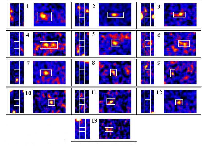
Figure 1.— 2D-spectra (in S/N units) of the 13 Ly$\alpha$ candidates (right panels) and the corresponding V-band image of the slit with the object positions (white boxes in left panels). The dispersion direction in the spectra is parallel to the x-axis. The scale of the panels is $32\mathrm{\AA}\times 10^{\prime\prime}$ for the spectra and $4^{\prime\prime}\times 10^{\prime\prime}$ for the images. The white boxes represent the apertures used to calculate the line and V-band flux. The values of flux and $1\sigma$ noise for each aperture is shown in Table 3 (see text for details).

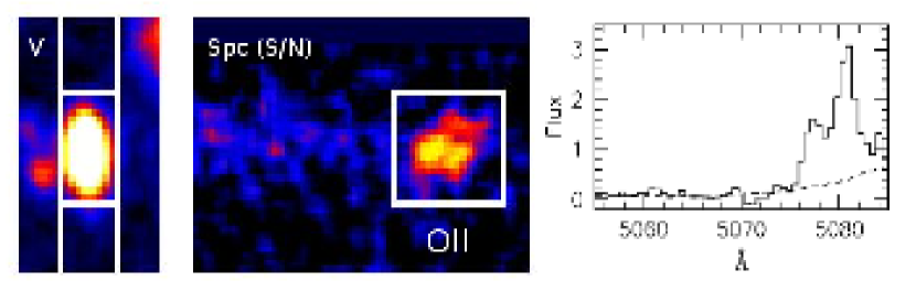
Figure 2.— V image (left panel), 2D-spectrum (in S/N units, central panel) and calibrated 1D-spectrum (solid histogram in right panel, dashed lines represent 1$\sigma$ errors) of a bright OII emitter ($m_{\mathrm{V}}\sim 17$) serendipitously found in one of our slits. The emission wavelength, the distance between peaks ($\sim 4\mathrm{\AA}$) and the flux ratio of the lines, all correspond to OII doublet at $z\sim 0.36$. The bright optical counterpart and the presence of a visible continuum redwards of the double emission line, also indicate that the emitter is a low-redshift galaxy.

Figure 3.— 1D calibrated spectra of the 13 Ly$\alpha$ candidates. The flux (in units of $10^{-18}$$\mathrm{erg}\ \mathrm{s}^{-1}\mathrm{cm}^{-2}\mathrm{\AA}^{-1}$ ) is obtained integrating within the aperture represented by the white boxes in the left panels of Fig.1. The dashed lines represent the 1$\sigma$ noise level.

Figure 4.— Observed surface brightness (SB) of the 13 Ly$\alpha$ candidates against their three-dimensional comoving distance from the quasar for two different quasar redshifts. The expected SB from self-shielded clouds, as calculated by the theoretical models of Paper I, is shown by the solid line. The total errors in the predicted SB should take into account the scatter around the model relation and the uncertainties on the derived value of the quasar luminosity ($L_{\rm LL}$) and spectral shape ($\alpha$). To give an idea of the effect of these uncertainties in the predicted SB we overplot the expected fluorescent SB for a Lyman Limit flux of $2\times L_{\rm LL}$ (upper dashed line) and $0.5\times L_{\rm LL}$ (lower dashed line). The limiting case of fluorescent emission from a static slab is represented by the dotted line. Open circles indicate the candidates with a V-band counterpart with flux greater than 1$\sigma$ for the correspondent photometric aperture (see text for details). The horizontal error bars take into account a peculiar velocity shift of $\pm 250$km s^-1. All the candidates with a SB equal or lower than the theoretical expectations curves are compatible with fluorescence induced by the quasar.

5. Discussion

Are any of our detected objects fluorescent? We know from §2 that a good fluorescent candidate should have: i) very high EW, ii) possibly (but not necessarily) a double-peaked profile, iii) a precise value of its SB. We would also like to see the number density of objects to roughly match the density calculated in §2, allowing for the uncertainty in clustering.

As a quick reference, we associated to each candidate in Table 3 a “+”(or “-”) if the corresponding indicator clearly suggests (or disfavors) a fluorescent origin for the Ly$\alpha$ emission. Regarding the first criterion we notice that, given the sensitivity limits of our V-band image, only the two brightest emitters (#1 and #2) have high upper limits to their EW (see Table 3) - and it would be extremely difficult to establish the required EW observationally. The low values of the EW for #3 and #6 indicate a likely non-fluorescent origin for the emission.

Two objects (#4 and #13) display a very clear signature of double-peaked emission. Candidate #4 is compatible with fluorescence if $\sigma_{\mathrm{th}}\sim 60$ km s^-1. Instead, object #13 is compatible both with fluorescent Ly$\alpha$ (with $\sigma_{\mathrm{th}}\sim 20$ km s^-1) and OII emission at $z=0.36$. However, the high EW, the intensity ratio of the peaks (i.e. that the blue peak is brighter than the red peak) all disfavor the association with [OII] emission.

The comparison of the expected fluorescent SB with the estimated SB of the individual candidates is shown in Fig. 4. Unfortunately the systemic redshift of the quasar is uncertain - $z=3.110$ is given by Osmer et al. 1994, and $z=3.123$ by Lanzetta et al. 1993. The expected SB from self-shielded clouds (solid line) is calculated from Eq. (1), using the corresponding value of L_LL ($\sim 10^{32}\mathrm{erg}\mathrm{s^{-1}}\mathrm{Hz^{-1}}$) and $\alpha$ ($0.61\pm 0.02$) for our quasar (extrapolated from Kuhn et al. 2001). Only the most distant objects (4, 5 and 6) have an estimated SB that is clearly too high to be due to fluorescence induced by the quasar, unless the quasar was brighter in the past. Note that two of these (5 and 6) both have $f_{\mathrm{V}}\gtrsim 1\sigma$ (and are represented by open-circle symbols in Fig. 4), and 6 in particular has already an EW that disfavors a fluorescent origin. In general, we can notice that the case $z_{\rm QSO}=3.110$ allows a better fit of the expected relation between SB and distance for the detected objects. In this case, at least $7-8$ candidates have a SB in good agreement with the theoretical expectations.

The theoretical curves shown in Fig. 4 are calculated assuming isotropic and time-invariant emission from the quasar. The candidates beyond the quasar could have been illuminated by a different UV flux with respect to the value measured by us. In particular, gas clouds at 20 comoving Mpc from the quasar (within which most of our candidates were found) should be responding to the ionizing flux of the quasar that was emitted or order $\sim 3\times 10^{7}$ yrs before the epoch of observation. At 40 comoving Mpc, where candidates #4, #5 and #6 lie, the time delay is two times larger, i.e. $\sim 6\times 10^{7}$ yrs, close to the expected life-time of the quasar (e.g. Porciani, Magliocchetti & Norberg 2004).

Turning the argument around, the effect of the time delay may represent a direct way to measure the radiative history of quasars, if the fluorescent origin of the sources can be proved. If we assume that our object #4 is truly fluorescent, which is plausible given the high EW and the clear double-peaked profile, its SB would provide us with direct proof that the quasar was shining $\sim 10^{8}$ yr ago with an ultraviolet luminosity 6-10 times higher than the present measurements. Confirmation of the fluorescent origin of object #4 would for this reason be especially interesting.

In conclusion, what we can say about the fluorescent nature of our detected objects? Unfortunately, there is no definitive evidence of fluorescence. The EW can be poorly constrained for most of our candidates, requiring extremely deep broad-band images (for ground observations). The SB-distance relation (as well as the emission-line profile), given all the theoretical and observational uncertainties discussed above, is only an approximate indicator.

Nevertheless, collecting all the indication so far, we can highlight 5 of the 13 objects which are most probably not fluorescent, i.e. #3 (low-EW), #5 (too high SB), #6 (both low-EW and too high SB), #11 and #12 (both objects are unresolved, in front of the quasar and with SB at the limit for fluorescence). However, given their higher upper limit on the EW (mainly because of their high line-flux) and their SB, objects #1 and #2 (if $z_{\rm QSO}=3.11$) could be good candidates for fluorescence. As noted above, object #4 could also be a good candidate, because the profile is flat in the center and the presence of a double-peaked profile, compatible with fluorescence if $\sigma_{\mathrm{th}}\sim 60$ km s^-1. Finally, objects #7, #8, #10, #12 and #13 have SBs compatible with fluorescent emission (for both quasar redshifts), but the EW is poorly constrained.

As a final remark, it is worth stressing that self-shielded fluorescent emitters around a quasar could also be detected in absorption as the equivalent of DLAs in the field (see §1 for further details). Therefore, the existence of such a fluorescent population could in principle support the association of DLAs with proto-galactic gas clouds (e.g. Haehnelt, Steinmetz & Rauch 1998). However, even if all fluorescent emitters around a quasar are DLAs, this does not imply the converse, allowing the possibility of a different origin for a part of these absorbing systems, like disk galaxies already in place (e.g. Prochaska & Wolfe 1998).

5.1. The number density of emitters

Given our sensitivity limits (SB${}_{\rm lim}\sim 10^{-18}$$\mathrm{erg}\ \mathrm{s}^{-1}\mathrm{cm}^{-2}\mathrm{arcsec}^{-2}$  for a typical aperture of $2^{\prime\prime}\times 2^{\prime\prime}$) and the assumed value of $L_{\rm LL}$ and $\alpha$ for our quasar, we can use the procedure discussed in §2 to derive the expected number of fluorescent and not-fluorescent sources in our volume. We find a physical number density of fluorescent emitters of $\mathrm{dN}/\mathrm{dV}\sim 0.3\pm 0.1$ Mpc^-3, detectable within $r_{\rm max}\sim 4.7$ physical Mpc from the quasar. Given the projected area covered by our slits in all three configurations ($\sim 1.4$ physical Mpc²), we therefore should be able to detect fluorescent emission within a total volume $V\sim 13$ physical Mpc³. The shape of this volume is approximatively a cuboid, being constrained from the limited field of view of the detector ($6^{\prime}.8\times 6^{\prime}.8$, corresponding to a physical Mpc scale of $3.2\times 3.2$ at this redshift). Therefore the number of expected fluorescent emitters within $r_{\rm max}$ from the quasar is $\sim 4\pm 1$. Notice, however, that this number does not take into account: (i) the expected enhancement of the number density of objects around the quasar due to clustering effects, (ii) any reduction due to beaming of the quasar emission - although we note that we would expect the illuminated cone to include the line of sight and thus to be more or less aligned with the accessible volume. In this context we looked to see whether foreground and background candidates were located on different sides of the quasar, possibly indicating beaming, but found no evidence of this.

By comparison, we expect $\sim 6$ non-fluorescent sources in our total sampled volume if it is similar to the radio galaxy environment studied by V05.

Despite the small statistics and with all the many uncertainties, these numbers agree very well with the detected number of objects in our survey. It may be a coincidence, but it is certainly consistent with the indication that about half of our detected sources may have a fluorescent origin.

6. Summary

Based on our recent model of fluorescent Ly$\alpha$ emission (Paper I), we carried out a Ly$\alpha$ survey around the $z\sim 3.1$ quasar QSO 0420-388 to search for signatures of fluorescence. We used a “multi-slit plus filter” technique to sparsely sample a volume of $\sim 14000$ comoving Mpc³ around the quasar (directly sampling $\sim 1700$ comoving Mpc³).

We found 13 emission line sources, selected on equivalent width, which are likely to be Ly$\alpha$ at a redshift close to the quasar. In order to try to distinguish fluorescent objects from internally ionized clouds, we measured three possible signatures of fluorescence: i) the line equivalent width, ii) the line profile, iii) the SB. We also calculated the expected number of fluorescent and non-fluorescent sources from theoretical models and recent Ly$\alpha$ surveys.

From a theoretical point of view, the best constraints would be a very high EW and, within some limitations, the relation of the SB with the distance from the quasar. Instead, the line profile cannot give precise information on the nature of the sources - a double-peaked profile is a possible indication of fluorescence, but it can be absent, or be present in non-fluorescent sources.

Unfortunately, given the current observational limits, there is at present no definitive evidence for fluorescence. There are good reasons to suspect that 5 objects are probably not-fluorescent, and this estimate is in good agreement with the number density of such sources around radio galaxies. Of the remaining 8 objects, two or three of them are quite good fluorescent candidates, based on moderately high upper limits to their EW, and, in some cases, the presence of extended emission with a flat SB and a double-peaked profile. The remaining $5-6$ candidates are consistent with fluorescence, but their upper-limits on the EW are low enough to provide little real constraint.

On the basis of our model (Paper I), we were expecting $3-5$ fluorescent sources in the inner region around the quasar, and, from other surveys of Ly$\alpha$ emitters around AGNs, we were expecting $\sim 6$ non-fluorescent sources in the total sampled volume. These estimates are certainly consistent with the idea that about half of our detected sources could be fluorescent.

In this case, the distance of most of the candidates from the ionizing source would imply that the quasar has been active for at least 30 Myr, with a UV luminosity similar (within a factor of a few) to the present day value. In particular, one of the best candidates for fluorescence is sufficiently far behind the quasar to imply a life-time of $\gtrsim 60$ Myr.

Although there are uncertainties in interpretation, due to both observational limitations and theoretical uncertainties (and no doubt a range of phenomena in Nature), the current study provides one of the first statistical samples of possible fluorescent emitters around a high-redshift quasar. Future studies on this category of objects will give information about the properties of proto-galactic clouds and, furthermore, on the emission properties (i.e. spatial and temporal variations) of high-redshift quasars.

References

- Adelberger et al. (2006) Adelberger, K. L., Steidel, C. C., Kollmeier, J. A., & Reddy, N. A. 2006, ApJ, 637, 74
- Antonucci (1993) Antonucci, R. 1993, ARA&A, 31, 473
- Bajtlik et al. (1988) Bajtlik, S., Duncan, R. C., & Ostriker, J. P. 1988, ApJ, 327, 570
- Bertin & Arnouts (1996) Bertin, E., & Arnouts, S. 1996, A&AS, 117, 393
- Bunker, Marleau, & Graham (1998) Bunker, A. J., Marleau, F. R., & Graham, J. R. 1998, AJ, 116, 2086
- Cantalupo et al. (2005) Cantalupo, S., Porciani, C., Lilly, S. J., & Miniati, F. 2005, ApJ, 628, 61
- Charlot & Fall (1993) Charlot, S., & Fall, S. M. 1993, ApJ, 415, 580
- Cowie & Hu (1998) Cowie, L. L., & Hu, E. M. 1998, AJ, 115, 1319
- Crampton & Lilly (1999) Crampton, D., & Lilly, S. 1999, ASP Conf. Ser. 191: Photometric Redshifts and the Detection of High Redshift Galaxies, 191, 229
- Francis & Bland-Hawthorn (2004) Francis, P. J., & Bland-Hawthorn, J. 2004, MNRAS, 353, 301
- Francis & McDonnell (2006) Francis, P. J., & McDonnell, S. 2006, MNRAS, 370, 1372
- Fynbo et al. (1999) Fynbo, J. U., Møller, P., & Warren, S. J. 1999, MNRAS, 305, 849
- Fynbo et al. (2003) Fynbo, J. P. U., Ledoux, C., Möller, P., Thomsen, B., & Burud, I. 2003, A&A, 407, 147
- Gould and Weinberg (1996) Gould, A. and Weinberg, D. H., 1996 ApJ, 468, 462
- Haardt & Madau (1996) Haardt, F., & Madau, P. 1996, ApJ, 461, 20
- Haehnelt et al. (1998) Haehnelt, M. G., Steinmetz, M., & Rauch, M. 1998, ApJ, 495, 647
- Hogan & Weymann (1987) Hogan, C. J. & Weymann, R. J. 1987, MNRAS, 225, 1P
- Kuhn et al. (2001) Kuhn, O., Elvis, M., Bechtold, J., & Elston, R. 2001, ApJS, 136, 225
- Lanzetta et al. (1993) Lanzetta, K. M., Turnshek, D. A., & Sandoval, J. 1993, ApJS, 84, 109
- Ledoux et al. (2003) Ledoux, C., Petitjean, P., & Srianand, R. 2003, MNRAS, 346, 209
- Le Fevre et al. (1996) Le Fevre, O., Deltorn, J. M., Crampton, D., & Dickinson, M. 1996, ApJ, 471, L11
- Lowenthal et al. (1990) Lowenthal, J. D., Hogan, C. J., Leach, R. W., Schmidt, G. D., & Foltz, C. B. 1990, ApJ, 357, 3
- Martinez-Gonzalez et al. (1995) Martínez-Gonzalez, E., Gonzalez-Serrano, J. I., Cayon, L., Sanz, J. L., & Martin-Mirones, J. M. 1995, A&A, 303, 379
- Neufeld (1990) Neufeld, D. A. 1990, ApJ, 350, 216
- Osmer et al. (1994) Osmer, P. S., Porter, A. C., & Green, R. F. 1994, ApJ, 436, 678
- Pascarelle et al. (1996) Pascarelle, S. M., Windhorst, R. A., Driver, S. P., Ostrander, E. J., & Keel, W. C. 1996, ApJ, 456, L21
- Pascarelle et al. (1998) Pascarelle, S. M., Windhorst, R. A., & Keel, W. C. 1998, AJ, 116, 2659
- Porciani, Magliocchetti & Norberg (2004) Porciani, C., Magliocchetti, M., & Norberg, P. 2004, MNRAS, 355, 1010
- Prochaska & Wolfe (1998) Prochaska, J. X., & Wolfe, A. M. 1998, ApJ, 507, 113
- Prochaska et al. (2003) Prochaska, J. X., Gawiser, E., Wolfe, A. M., Castro, S., & Djorgovski, S. G. 2003, ApJ, 595, L9
- Schaerer (2003) Schaerer, D. 2003, A&A, 397, 527
- Schlegel et al. (1998) Schlegel, D. J., Finkbeiner, D. P., & Davis, M. 1998, ApJ, 500, 525
- Simcoe et al. (2004) Simcoe, R. A., Sargent, W. L. W., & Rauch, M. 2004, ApJ, 606, 92
- Steidel et al. (2000) Steidel, C. C., Adelberger, K. L., Shapley, A. E., Pettini, M., Dickinson, M., & Giavalisco, M. 2000, ApJ, 532, 170
- Taniguchi et al. (2003) Taniguchi, Y., Shioya, Y., Ajiki, M., Fujita, S. S., Nagao, T., & Murayama, T. 2003, Journal of Korean Astronomical Society, 36, 123
- Venemans et al. (2005) Venemans, B. P., et al. 2005, A&A, 431, 793
- Wolfe et al. (1995) Wolfe, A. M., Lanzetta, K. M., Foltz, C. B., & Chaffee, F. H. 1995, ApJ, 454, 698
- Zwaan & Prochaska (2006) Zwaan, M. A., & Prochaska, J. X. 2006, ApJ, 643, 675