Characterization of Gravitational Microlensing Planetary Host Stars

Abstract

The gravitational microlensing light curves that reveal the presence of extrasolar planets generally yield the planet-star mass ratio and separation in units of the Einstein ring radius. The microlensing method does not require the detection of light from the planetary host star. This allows the detection of planets orbiting very faint stars, but it also makes it difficult to convert the planet-star mass ratio to a value for the planet mass. We show that in many cases, the lens stars are readily detectable with high resolution space-based follow-up observations in a single passband. When the lens star is detected, the lens-source relative proper motion can also be measured, and this allows the masses of the planet and its host star to be determined and the star-planet separation can be converted to physical units. Observations in multiple passbands provide redundant information, which can be used to confirm this interpretation. For the recently detected super-Earth planet, OGLE-2005-BLG-169Lb, we show that the lens star will definitely be detectable with observations by the Hubble Space Telescope (HST) unless it is a stellar remnant. Finally, we show that most planets detected by a space-based microlensing survey are likely to orbit host stars that will be detected and characterized by the same survey.

1 Introduction

One of the primary strengths of the gravitational microlensing extrasolar planet detection method is its sensitivity to low-mass planets at separations of a few AU. This has recently been demonstrated with the discovery of two of the lowest mass extrasolar planets known: OGLE-2005-BLG-390Lb, a $5.5{+5.5\atop-2.7}M_{\oplus}$ planet orbiting an M-dwarf in the Galactic bulge (Beaulieu et al., 2006), and OGLE-2005-BLG-169Lb, a $13{+6\atop-8}M_{\oplus}$ which probably orbits a K or early M star in the inner Galactic disk (Gould et al., 2006). Both of these planets have a separation from their host star of about $\sim 3\,$AU, and this places them well outside the current sensitivity range of the radial velocity method, which is only sensitive to such planets with a separation of $\lower 2.15277pt\hbox{$\;\buildrel<\over{\sim}\;$}0.7\,$AU (Rivera et al., 2005; Lovis et al., 2006).

The microlensing method is most sensitive to planets at a separation of 1-5 AU, and this separation region is particularly interesting from a theoretical point of view because it contains the so-called “snow-line” which is an important feature for the core accretion theory of planet formation. This “snow-line” is the region of the proto-planetary disk where it is cold enough for water-ice to condense, and the core accretion theory predicts that this is where the most massive planets will form (Ida & Lin, 2004; Laughlin, Bodenheimer & Adams, 2004; Kennedy et al., 2006). According to this theory, giant planets form just outside the “snow line” where they can accrete $\sim 10M_{\oplus}$ of rock and ice to form a core that grows into a gas giant like Jupiter or Saturn via the run-away accretion of Hydrogen and Helium onto this core. However, this theory also predicts that the Hydrogen and Helium gas can easily be removed from the proto-planetary disk during the millions of years that it takes to build the rock-ice core of a gas-giant. Thus, if the core accretion theory is correct, rock-ice planets of $\sim 10M_{\oplus}$ that failed to grow into gas giants should be quite common. Recent core-accretion theory calculations (Laughlin, Bodenheimer & Adams, 2004; Ida & Lin, 2004; Boss, 2006a) predict that it is especially difficult to form gas-giant planets around low-mass stars.

As of November, 2006, there have been four extrasolar planets discovered by the microlensing method: two planets more massive than Jupiter (Bond et al., 2004; Udalski et al., 2005) in addition to the two $\sim 10M_{\oplus}$ super-Earth planets. But, the microlensing planet detection efficiency is more than an order of magnitude larger for Jupiter-mass planets than for $10M_{\oplus}$ planets, so the microlensing results indicate that planets of $\sim 10M_{\oplus}$ are significantly more common than Jupiters (Beaulieu et al., 2006) and that 16-69% (90% c.l.) of non-binary stars have a planet of $\sim 10M_{\oplus}$ (Gould et al., 2006) at a separation of $\sim 1.5$-4 AU. The discovery of these two planets suggests that super-Earth planets of $\sim 10M_{\oplus}$ are more common than Jupiter mass planets at separations of a few AU around the most common stars in our Galaxy. This would seem to confirm a key prediction of the core accretion model for planet formation: that Jupiter mass planets are much more likely to form in orbit around G and K stars than around M stars (Laughlin, Bodenheimer & Adams, 2004; Ida & Lin, 2004), although super-Earth planets are also predicted in the gravitational instability model (Boss, 2006b). In fact, (Laughlin, Bodenheimer & Adams, 2004) have argued that the Jupiter-mass planets found in microlensing events (Bond et al., 2004; Udalski et al., 2005) are more likely to orbit white dwarfs than M dwarfs. Clearly, the microlensing detections would provide tighter constraints on the theories if the properties of the host stars were known.

In this paper, we show that the planetary host stars can often be identified in high resolution images taken a few years after the microlensing event. In cases where the lens star has been identified, we show in § 2 that a complete solution to the microlensing event can generally be found. The complete solution gives the lens star and planet masses and the separation in physical units instead of just the star-planet mass ratio and separation in Einstein ring radius units. This has recently been demonstrated with the first planet discovered by microlensing, OGLE-2003-BLG-235Lb/MOA-2003-BLG-53Lb (Bennett et al., 2006), and in § 3, we consider the more favorable case of the low-mass planetary microlensing event OGLE-2005-BLG-169, where the lens star will be detectable if it is a main sequence star of any mass. In § 4, we show that a space-based microlensing survey (Bennett & Rhie, 2002), like the proposed Microlensing Planet Finder (MPF) mission (Bennett et al., 2004) will detect the planetary host stars for most of the detected planets, and so, planets detected by MPF will usually come with a complete solution of the lens system. We conclude, in § 5, with a discussion of follow-up observations of planetary microlensing events and argue that the host stars will generally be detectable unless they are stellar remnants or brown dwarfs.

2 Lens-Source Relative Proper Motion and Complete Solution of Microlensing Events

Gravitational microlensing can be used to study objects, such as brown dwarfs, stellar remnants, or extrasolar planets that emit very little detectable radiation, but most microlensing events provide only a single parameter, the Einstein radius crossing time, $t_{E}$, that can constrain the lens system mass, distance, and velocity. The situation is significantly improved when the lens-source relative proper motion, $\mu_{\rm rel}$, can be determined, because this yields the angular Einstein radius: $\theta_{E}=\mu_{\rm rel}t_{E}$. The angular Einstein radius is related to the lens system mass by

$$M_{L}={c^{2}\over 4G}\theta_{E}^{2}{D_{S}D_{L}\over D_{S}-D_{L}}\ ,$$ (1)

where $D_{L}$ and $D_{S}$ are the lens and source distances, respectively. $M_{L}=M_{\ast}+M_{p}$ is the total lens system mass: the sum of the star and planet masses. Since $D_{S}$ is known (at least approximately), eq. 1 can be considered to be a mass-distance relation for the lens star.

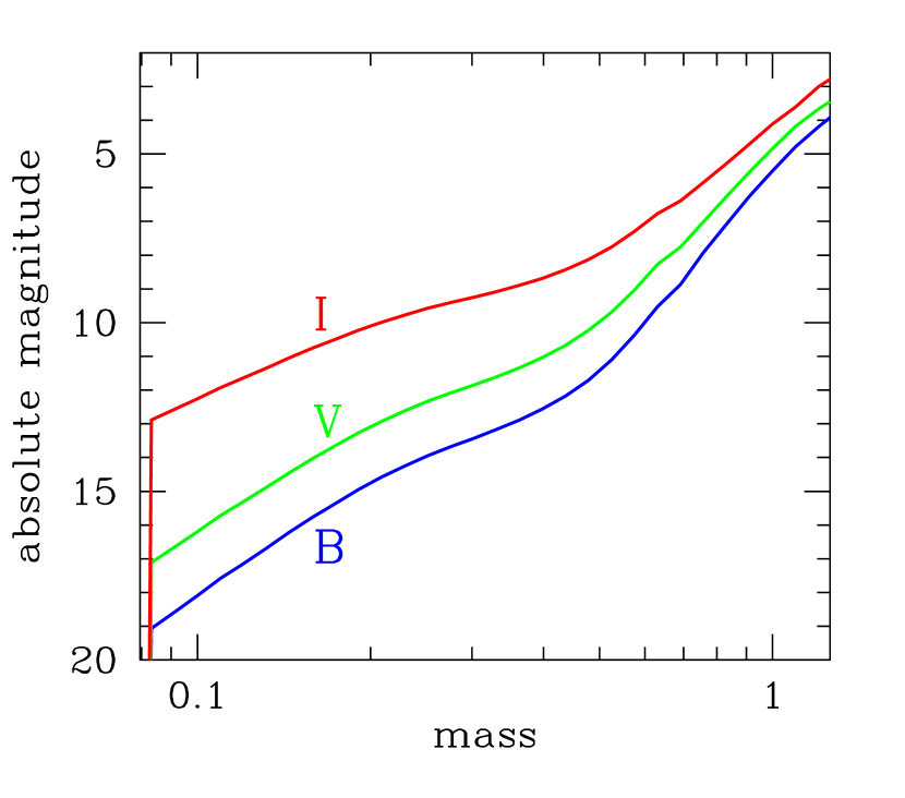
Figure 1: The adopted mass-luminosity relations in the I (F814W), V (F555W), and B (F435W) passbands. These an empirical mass-luminosity relations (Kroupa & Tout, 1997) extended to higher masses and the $B$-band using Drilling & Landolt (2000), Schmidt-Kaler (1982) and Gray (1992). Approximately Solar metallically is appropriate for the lens stars in the inner Galactic disk and the bulge.

Another constraint on the lens system is needed in order to convert this mass-distance relation to a complete solution of the lens event. For most events, this can be accomplished by direct detection of the planetary host star. If the brightness of the host (lens) star is measured, then the mass-distance relation, eq. 1, can be combined with a mass-luminosity relation, such as those shown in Figure 1, to yield the mass of the lens system. This then allows the individual star and planet masses to be determined, since the mass ratio is known from the microlensing light curve. This also allows the separation determined from the light curve to be converted from units of the Einstein radius, $R_{E}$, to physical units.

There is still some residual uncertainty due to the uncertainty in $D_{S}$, but this is generally small as can be illustrated with some special cases. If $D_{L}\ll D_{S}$, then eq. 1 indicates that $M_{L}$ becomes independent of $D_{S}$. In the opposite extreme, with the lens very close to the source ($D_{L}\approx D_{S}$), we can treat $D_{S}$ and $D_{S}-D_{L}$ as the independent variables and replace $D_{L}$ by $D_{S}$ (except in the expression $D_{S}-D_{L}$), so in this limit $M_{L}\propto D_{S}^{2}/(D_{S}-D_{L})$ The mass luminosity relations shown in Figure 1 can be approximated by a power law over a limited range of masses. So, if we take ${\cal L}\propto M^{n}$ as our mass-luminosity relation, the lens mass is simply given by $M_{L}\propto F_{L}^{1/n}D_{S}^{2/n}$, where $F_{L}$ is the measured flux of the lens star. (Eq. 1 then gives $D_{S}-D_{L}$ in terms of $M_{L}$.) Since the appropriate value of $n$ is almost always $n>2$, the fractional error in $M_{L}$ due to the uncertainty in $D_{S}$ will generally be smaller than the fractional uncertainty in $D_{S}$.

It is important to note that this complete solution of the lens system requires only the lens brightness in a single pass-band. Color information obtained by multi-band observations is redundant, and can be used to constrain the possibility that the source or lens star has a bright binary companion.

An alternative method for the complete solution of a microlensing event is to combine a measurement of the lens-source proper motion with a measurement of the microlensing parallax effect. This has already been demonstrated for microlensing events due to single stars (Drake, Cook, & Keller, 2004; Gould, Bennett, & Alves, 2004) and stellar binaries (An et al., 2002). The detection of the microlensing parallax effect provides a measurement of $\tilde{r}_{e}$, the projected Einstein radius (projected from the position of the source to that of the observer). As originally shown by Gould (1992), the measurement of both $\theta_{E}$ and $\tilde{r}_{e}$ yields the lens system mass,

$$M_{L}={c^{2}\over 4G}\tilde{r}_{e}\theta_{E}\ ,$$ (2)

without any dependence on $D_{S}$ or $D_{L}$. However, $\tilde{r}_{e}$ is generally measured by detecting the effect of the Earth’s orbital motion in the light curve (Alcock et al., 1995), and this means that reliable measurements of $\tilde{r}_{e}$ can generally only be made for very long duration events or events where the lens-source motion is unusually small (Alcock et al., 2001b; Drake, Cook, & Keller, 2004; Gould, Bennett, & Alves, 2004; An et al., 2002; Mao, 1999; Smith et al., 2002; Bond et al., 2001; Bennett et al., 2002; Poindexter et al., 2005). For shorter events, the light curve may reveal only a single component of the two-dimensional ${\bf\tilde{r}_{e}}$ vector. It is then possible to determine the lens mass from eq. 2 if the direction of ${\mbox{\boldmath$\bf\mu$}_{\rm rel}}$ is measured, since these two vectors are parallel.

2.1 Lens-Source Relative Proper Motion Determination Methods

There are two methods of measuring the relative proper motion. The first involves a measurement of finite source effects in the microlensing light curve combined with an estimate of the angular size of the source. These finite source effects are commonly detectable in binary lens events (Mao & Paczyński, 1991), when the angular position of the source crosses or comes very close to the caustic curve of the lens (Bennett et al., 1996; Afonso et al., 2000; Alcock et al., 2000; Jaroszynski et al., 2005). Finite source effects are particularly common in planetary microlensing events because the planet is likely to be detected only if the source crosses or closely approaches the caustic curve. In fact, all four planetary microlensing events observed to date (Bond et al., 2004; Udalski et al., 2005; Beaulieu et al., 2006; Gould et al., 2006) have revealed finite source effects, which reveal the source crossing time, $t_{\ast}$. The angular radius of the source star, $\theta_{\ast}$, can be estimated from its color and brightness. This yields the relative proper motion, $\mu_{\rm rel}=\theta_{\ast}/t_{\ast}$, and the angular Einstein radius, $\theta_{E}=\theta_{\ast}t_{E}/t_{\ast}$, because $t_{E}$ can virtually always be determined from the light curve of planetary microlensing events.

Even if the light curve does not reveal any finite source effects, it is still possible to measure $\mu_{\rm rel}$ directly by detecting the lens star and measuring the lens-source separation as was done for microlensing event MACHO-LMC-5 (Alcock et al., 2001b). For this event, the relative proper motion was quite large, $\mu_{\rm rel}=21.4\,$mas/yr, because the distance to the lens is small, $D_{L}=550\,$pc. As a result, the lens and source were easily resolved in HST images taken 6.3 years after peak magnification.

Galactic bulge microlensing events with planetary signals generally have relative proper motions that are much smaller than this, typically, $\mu_{\rm rel}\sim 5\,$mas/yr. Thus, the lens stars would typically not be resolved in HST images taken less than a decade after peak magnification. But, due to the stability of the HST point-spread function (PSF), it is possible to measure lens-source separations that are much smaller than the width of the PSF. This is accomplished by measuring the elongation of the combined lens-source image due to the fact that it consists of two point sources instead of one.

2.2 Image Elongation

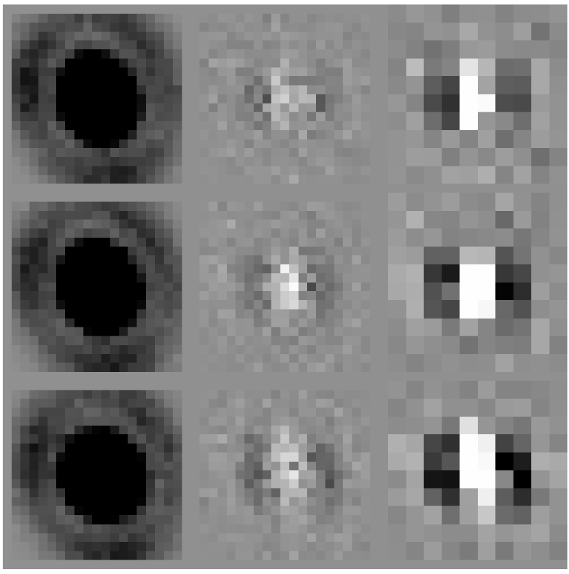
Figure 2: Simulated image stacks of multiple dithered exposures of the OGLE-2005-BLG-169 source and lens star 2.4 years after peak magnification using the HST/ACS High Resolution Camera (HRC) in the F814W filter band. The top row of images assumed a host star mass of $M_{\ast}=0.08M_{\odot}$, the middle row assumes $M_{\ast}=0.35M_{\odot}$, and the bottom row assumes $M_{\ast}=0.63M_{\odot}$. In each row, the image on the left shows the raw image stack sampled at one half the native HRC ($28\,$mas) pixel size. The central column shows the residuals after subtraction of the best fit PSF model, showing the blended image elongation along the $x$-axis due to the lens-source separation. The right hand column shows these residuals rebinned to the $28\,$mas native pixel scale.

Figure 2 shows a simulated images from the Hubble Space Telescope (HST) Advanced Camera for Surveys (ACS) of the source and lens star for microlensing event OGLE-2006-BLG-169 taken 2.4 years after peak magnification when the lens-source separation is predicted to be $20.2\pm 1.7\,$mas. These simulated images represent the co-added dithered exposures from a single orbit of observations in the $I$-band (F814W), and the three different rows of images represent three possible masses for the planetary host star. While the $20.2\pm 1.7\,$mas lens-source separation is smaller than the diffraction limited $I$-band PSF FWHM of $\sim 76\,$mas, the elongation of the PSF of the blended source-lens star pair is clearly visible in the residual images shown in the central and right hand columns.

The high precision image elongation measurements that we desire depend on a precise knowledge of the PSF, but this is to be expected with space-based observations of microlens source stars. The Galactic bulge fields where microlensing events are discovered have large numbers of relatively bright, but reasonably well separated stars in the field of the lens, and this enables the determination of very accurate PSF models, as long as the space telescope observations are dithered to correct for image undersampling. Prior HST programs have demonstrated that HST has the requisite image stability (Lauer, 1999; Anderson & King, 2000, 2004).

There is a potential degeneracy encountered when converting the image elongation into a value for the lens-source displacement. The elongated image full-width half-maximum (FWHM) in the direction of the lens-source separation is determined by the lens-source separation and their brightness ratio. Thus, if we only measure the increased FWHM of the elongated image, we won’t be able to determine the brightness ratio and the separation. Fortunately, the microlensing light curves with definitive planetary signals will generally provide the information needed to break this degeneracy. These light curves have sufficient high precision photometry to determine the brightness of the source star from the shape of the microlensing light curve. Furthermore, most planetary light curves also exhibit finite source effects, which allow an independent determination of the lens-source relative proper motion, $\mu_{\rm rel}$. For these events, we can consider the image elongation to be a measure of the the brightness ratio, which can be compared to the source star brightness from the light curve as a test for a bright binary companion to the source star.

The most reliable way to estimate the precision of our measurement of $\mu_{\rm rel}$ is with Monte Carlo simulations using realistic PSF models, which are well understood in the case of HST. However, it is instructive two consider a much simpler procedure. Let $\Delta x$ be the lens-source separation at a time, $T$, after peak magnification. The relative proper motion is therefore $\mu_{\rm rel}=\Delta x/T$. If we approximate the PSF with a Gaussian profile, $e^{-0.5x^{2}/s_{0}^{2}}$, then the blended image of the source plus lens star will be represented by the sum of two Gaussian profiles with centers separated by $\Delta x$. We can then approximate this sum of Gaussians with a broader Gaussian, $e^{-0.5x^{2}/s^{2}}$, where we require that the broader Gaussian has the same RMS value as the original sum of Gaussians (in the direction of the lens-source proper motion). This yields

$$s^{2}=s_{0}^{2}+f_{L}(1-f_{L})(\Delta x)^{2}\ ,$$ (3)

where $f_{L}=F_{L}/F_{\rm tot}$ is the ratio of the flux of the lens to the total flux in the PSF. Since the source flux $F_{S}=F_{\rm tot}-F_{L}$ is known from the light curve, and $F_{\rm tot}$ can be measured from the images being analyzed, we can consider $f_{L}$ to be known from the light curve. The uncertainties in the lens-source separation, $\Delta x$, and relative proper motion, $\mu_{\rm rel}$ can be derived,

$$\frac{\sigma_{\Delta x}}{\Delta x}=\frac{\sigma_{\mu}}{\mu_{\rm rel}}=\frac{1}{\sqrt{2N_{tot}}}\left(\frac{s_{0}^{2}}{f_{L}(1-f_{L})(\Delta x)^{2}}\right)\ .$$ (4)

Here $N_{tot}$ is the total number of photons in the PSF. We find that eq. 4 does an excellent job of describing the precision of our simulated $\Delta x$ measurements for a variety of model PSFs, although in some cases, it may be necessary to multiply eq. 4 by a fudge factor (to account for the inadequacies of our Gaussian approximation).

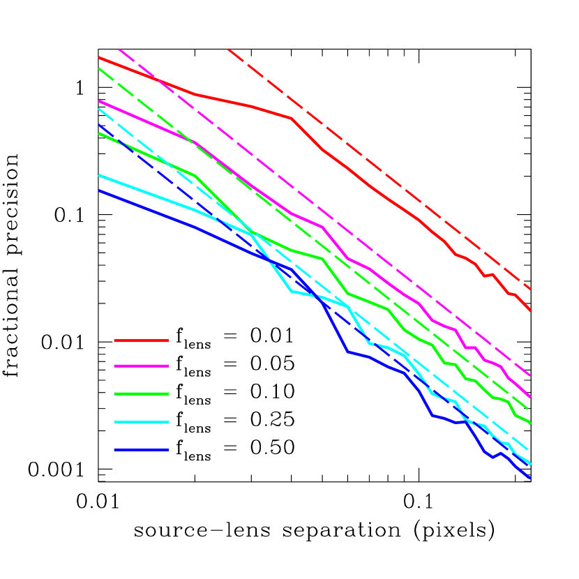
Figure 3: The uncertainty in the lens-source separation, $\Delta x$, is shown as a function of $\Delta x$. The different colors indicate different fractions, $f_{L}$ of the blended lens plus source light that is due to the lens. Solid lines indicate the results of our simulations, and dashed lines are calculated from eq. 4. These estimates assume a total of $10^{8}$ detected photons from the blended lens plus source.

This approximate formula is compared to the actual uncertainties, derived from our simulations in Figure 3 for parameters appropriate for a space-based microlensing survey, such as the proposed Microlensing Planet Finder (MPF) mission (Bennett et al., 2004). (Such a mission would have a PSF FWHM 2-3 times worse than HST, but would have the ability to combine images with a combined exposure time of months.)

We expect that eq. 4 may fail to describe the measurement uncertainty for $\Delta x$ when the lens-source separation grows to $\Delta x\lower 2.15277pt\hbox{$\;\buildrel>\over{\sim}\;$}s_{0}$ and the lens and source images begin to be separately resolved in the high resolution images. In this case, there are more features of the image that can aid in the determination of $\Delta x$, so we should be able to measure $\Delta x$ even better than eq. 4 predicts. However, this is only likely to occur in cases where $\sigma_{\Delta x}$ is already quite small, and so eq. 4 will simply give a very conservative estimate of $\sigma_{\Delta x}$ in these cases.

For most planetary events, the light curve shows finite source effects that allow $t_{\ast}$ and therefore $\mu_{\rm rel}$ and $\Delta x$ to be determined from the light curve. In these cases, the image elongation can be used to measure $f_{L}$, and the uncertainty in the $f_{L}$ determination is given by

$$\sigma_{f_{L}}=\sqrt{\frac{2}{N_{tot}}}\left(\frac{s_{0}}{\Delta x}\right)^{2}\frac{1}{|1-2f_{L}|}\ .$$ (5)

In most cases, this determination of $f_{L}$ will be redundant with the determination from the light curve fit and the total lens plus source flux. However, if the source star has a bright binary companion, at a separation $>10\,$ so that the light curve is not affected, then these two methods will yield different results. The binary companion will contribute to the $F_{S}=F_{\rm tot}(1-f_{L})$ value as measured by image elongation, but it will not contribute to the value of $F_{S}$ determined from the light curve. Thus, the different measures of $F_{S}$ provide a measurement of the brightness of the source star’s binary companion.

In order to determine how precisely we can measure both $\Delta x$ and $f_{L}$ from the blended image of the source plus lens, we will need to measure the third moment, or skewness, of the blended image profile. The third moment is given by

$$Q={1\over N_{tot}}\sum(x-x_{0})^{3}\ ,$$ (6)

where the sum is over the positions of the detected photons and $x_{0}$ is the mean position of the detected photons. If the image profile is approximately a Gaussian, then $Q$ can be measured to a precision of $\sigma_{Q}=s^{3}\sqrt{15/N_{tot}}$. We can also derive the following expression for $Q$ in terms of $f_{L}$ and $\Delta x$,

$$Q=f_{L}(1-f_{L})(1-2f_{L})(\Delta x)^{3}\ .$$ (7)

This expression can be used to derive the following expressions for the uncertainties in $f_{L}$ and $\Delta x$ when we solve for both,

$$\frac{\sigma_{\Delta x}}{\Delta x}\approx\sqrt{15\over N_{tot}}{1\over f_{L}}\left({s\over\Delta x}\right)^{3}\ ,$$ (8)

and

$$\sigma_{f_{L}}\approx\sqrt{60\over N_{tot}}\left({s\over\Delta x}\right)^{3}\ .$$ (9)

These expressions assume that $f_{L}\ll 1$ and that the uncertainties are dominated by our ability to measure $Q$, which will generally be the case when $\Delta x/s\lower 2.15277pt\hbox{$\;\buildrel<\over{\sim}\;$}1$.

An additional complication is the possibility of blending by stars that played no role in the microlensing event, which happen by chance to lie close to the positions of the source and lens stars. However, the mean separation of stars in the Galactic bulge fields that are searched for microlensing events is in the range of 0.3-1.0 arc seconds, which is much larger than the lens-source separations. Thus, if the lens-source star separation can be measured, it is unlikely that stars unrelated to the microlensing event will interfere significantly with the lens-source separation measurement. The only exception would be stars that are physically associated with the lens or source stars, and this possibility is dealt with in § 2.5 below. For a space-based microlensing survey, it should generally be possible to directly detect the unrelated blended stars with a point-source decomposition algorithm. (This is similar to deconvolution (Magain et al., 2006) except that it makes use of the fact these Galactic bulge field contain very few sources that are not point-like.)

We should also note that this estimate of our ability to measure the separation of two unresolved stars is substantially better than the conservative estimate of Han et al. (2006). Our estimate is justified by our detailed simulations, which are, in turn, based on experience with HST data (Anderson & King, 2004). Thus, we are confident that the conservative assumptions of Han et al. (2006) are not needed.

2.3 Color Dependent Centroid Offset

Another method to detect the effects of the relative lens-source proper motion relies upon the likelihood that the lens and source will have different colors. This means that the lens star will contribute a different fraction to the total light seen in the source plus lens image blend as seen in different passbands. This magnitude of the observed color-dependent image center shift for the $V$ and $I$ passbands is

$$\Delta x_{V-I}=\left(f_{I}-f_{V}\right)\Delta x\ .$$ (10)

$\Delta x_{V-I}$ is directly measurable from high resolution HST images, but $f_{I}$ and $f_{V}$ depend on brightnesses of the lens and source in both passbands. The brightness of the source star in multiple passbands can generally be obtained by multicolor observations at several different magnifications during the course of the microlensing event, but the brightness of the lens star is an unknown that must be solved for along with $\Delta x$. Equations 1 and 10 can be combined with the $V$ and $I$ band mass-lumonisity relations shown in Figure 1 to yield four equations for the four unknowns: $M$, $V_{L}$, $I_{\rm lens}$, and $\Delta x=\theta_{E}T/t_{E}$. These equations can then be solved to yield a complete solution for the microlensing event parameters. This effect has been detected for the first extrasolar planet discovered by microlensing (Bennett et al., 2006), but in this case, $\mu_{rel}$ (and therefore $\theta_{E}$ and $\Delta x$) was already known from the microlensing event light curve.

An important advantage of this method is that for small $\Delta x$, the signal is $\propto\Delta x$. Thus, as long as the colors of the source and lens stars differ significantly, this method should measure small $\Delta x$ vlaues more precisely than the image elongation method.

2.4 Interstellar Extinction

Because our methods involve measuring the brightness and color of the planetary host star in the direction of the Galactic bulge, interstellar extinction is an important consideration. Extinction affects the determination of the brightness and color of both the source and lens stars. The angular radius of the source star, $\theta_{\ast}$, is determined from its brightness and color, and $\theta_{\ast}$ is used to determine the lens-source relative proper motion, $\mu_{\rm rel}$, and the angular Einstein radius, $\theta_{E}$. Fortunately, extinction makes stars appear both fainter and redder, and these two effects push our estimate of $\theta_{\ast}$ in opposite directions. As a result, our estimate of $\theta_{\ast}$ is not highly dependent on the uncertainty in our extinction estimate.

The dust in the Galactic disk is generally modeled with a disk scale height of $\sim 100\,$pc (Drimmel & Spergel, 2001). Since the source and lens stars are generally located at a distance $\lower 2.15277pt\hbox{$\;\buildrel>\over{\sim}\;$}1$-2 kpc, and are $\lower 2.15277pt\hbox{$\;\buildrel>\over{\sim}\;$}2^{\circ}$ from the Galactic plane, the extinction is primarily in the foreground of both the source and lens star. The extinction toward the Galactic bulge is also quite patchy, so it cannot be reliably estimated by a simple model. Instead, the standard practice for the interpretation of microlensing events is the estimate the extinction toward the source based upon the observed colors and magnitudes of stars within 1-2 arc minutes of the microlensed source (Bond et al., 2004; Udalski et al., 2005; Beaulieu et al., 2006; Gould et al., 2006). For the lens star, the extinction must be modeled with a probability distribution, which matches the measured extinction at the distance of the source and follows the exponential scaling of Drimmel & Spergel (2001). The variance of the probability distribution accounts for the patchiness of the actual distribution. In practice (Bennett et al., 2006), this procedure amounts to only a slight modification to the simpler case in which all the extinction is assumed to lie in the foreground of both the lens and source. For simplicity, in this paper, we will assume that extinction for the lens is identical to the extinction for the source star, and we will not explicitly discuss the extinction in the remainder of this paper.

2.5 Binary Companions to the Lens or Source

Although binary stars represent a minority of star systems (Lada, 2006), it is important to consider the effect of a binary source or lens star on our analysis of the planetary host star properties. A binary companion to the lens or source star would generally be unresolved from the source, so it would complicate our analysis. But, such a possibility is also constrained by the properties of the microlensing light curve.

A binary companion to the source star can often be detected via light curve oscillations due to orbital motion of the source star if the orbital period is less than a year (Derue et al., 1999; Alcock et al., 2001a). Microlensing events with main sequence source stars and detected planetary light curve features generally have a peak magnification of $A_{\rm max}\lower 2.15277pt\hbox{$\;\buildrel>\over{\sim}\;$}10$ because lower magnification events typically have poor photometry due to the crowding in ground-based images. If the event is well sampled near peak magnification, binary source effects in the light curve will be visible with an amplitude of $\sim a/(R_{E}A_{\rm max})$, where $a$ is the semi-major axis of the source star orbit. For $A_{\rm max}>10$, this implies that even the orbital motion of a contact binary will be visible if the photometric precision is close to 1%. Thus, in most cases, a binary companion to the source must have a semi-major axis $\lower 2.15277pt\hbox{$\;\buildrel>\over{\sim}\;$}1\,$AU in order to avoid visible light curve effects. If the source star’s companion is not much fainter than the source, then the lensing of the companion star may be visible in the light curve unless the source-companion separation is $\lower 2.15277pt\hbox{$\;\buildrel>\over{\sim}\;$}R_{E}\sim$ several AU. If the separation of the source from its companion is $\lower 2.15277pt\hbox{$\;\buildrel>\over{\sim}\;$}5$-$10\,$mas, depending on its brightness, then we will be able distinguish its position from that of the source star using the same methods that we have discussed to detect the lens-source offset. For a typical bulge source distance of $9\,$kpc, this corresponds to a source-companion separation of 45-$90\,$AU, so for separations larger than this, the binary companion will affect our measurements of lens-source astrometry.

The light curve constraints on a possible companion to the lens and planetary host star depend more sensitively on the parameters of the specific microlensing event. For a very high magnification event, such as OGLE-2005-BLG-169 (see § 3), a companion of similar mass to the planetary host star can be excluded over a very wide range of separations from $\sim 0.01$-$100R_{E}$ or $\sim 0.03$-$300\,$AU. For events of more modest magnification, the binary separations are excluded over a more modest range of separations, $\sim 0.1$-$10R_{E}$. So, there will usually be at least a slim chance of the lens star system is a close binary star system with a semi-major axis $a\ll 1\,$AU or a wide binary system with $a\gg 1\,$AU. The observational signature of a wide binary companion is similar to the signature of a binary companion to the source in that there is an extra source of light located very close to the positions of the lens and source. However, this extra source will move with the planetary host star, and so the image elongation signal will be stronger. In contrast, if the planetary host star is a close binary, then both stars will contribute the lens mass in eq. 2, so the lens star system will be fainter and redder than implied by the single-star mass-luminosity functions shown in Figure 1.

2.6 Full Solution with Combined High Resolution Follow-up Data

One complication that may tend to interfere with the recovery of the planetary host star parameters is the possibility that either the source star or the planetary host star will have a binary companion star that contributes a significant amount of flux to the blended image. Such a star would generally be unresolved from the position of the lens and source star, and this would hamper our ability to recover the brightness of the lens star. Generally, such a binary companion to the source or lens star would have to have a separation $\gg 10\,$AU from the lens or source to avoid an obvious light curve signal. For high magnification microlensing events, a binary companion would have to have an even larger separation to avoid detection, but for a low magnification event, it would be possible to find a planet orbiting a very close binary star system with no detectable light curve features. Fortunately, the high resolution follow-up data provides more than enough constraints to identify these binary companions, in most cases.

The critical unknown parameters for a microlensing event are the lens mass, distance and relative proper motion, $\mu_{rel}$, and these are constrained by the light curve parameters $t_{E}$ and $t_{\ast}$ (which is usually, but not always, measured). The light curve also yields the source star brightness, usually in two different pass bands, but these measurements can only constrain the lens star parameters in conjunction with the high resolution images. With deep, two-color high resolution space-based follow-up observations, it is possible to measure five additional parameters: the source plus lens brightness in two colors, the image elongation in two colors, and the source plus lens centroid offset between the two colors. In all, we have 8-9 constraints for the 3 microlensing event unknowns, so the problem is significantly over-constrained.

These 5-6 additional parameters can be used to constrain other possibilities, such as a bright binary companion to the lens or source star. Such a companion would add 1 parameter (the companion mass) to the problem or possibly three parameters if the separation of the companion is large. We could probably constrain a companion to the lens, source or both with these 5-6 additional parameters. However, the best way to solve a lens system that involves a bright, distant lens or source companion would be to obtain high resolution space-based images at multiple epochs. This would add four additional measured parameters and allow us to distinguish stellar separation due to the lens-source relative proper motion from the separation of a distant binary companion to the lens or source.

Of course, we haven’t shown that these parameters will always be measured to sufficient precision to guarantee a complete lens solution. A complete investigation of this question is beyond the scope of the present paper, but we will demonstrate that the question of binaries is easily resolved for the example event that we discuss in § 3. Also, because $\Delta x$ grows with time, the precision of our measurements will grow with time, so it is likely that many ambiguities can be resolved with additional follow-up observations. Thus, we can generally expect a complete solution of the microlensing event when light from the lens can be observed by HST or another high angular resolution spaced-based telescope.

In practice, some of these measurements can have significant or correlated uncertainties, so the observational constraints are best applied through a Bayesian analysis. In fact, such an analysis is able to provide relatively precise event parameters even without even observational constraints to constrain binary companions to the source and lens, because the a priori probability of a binary companion of similar brightness to the source is relatively small. For example, in the case of the first microlensing planet discovery Bennett et al. (2006) were able to constrain the host star mass to an accuracy of about $13\,$%.

3 A Low-Mass Planetary Event with a Detectable Lens Star

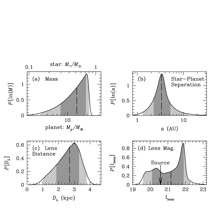
Figure 4: Bayesian probability densities for the properties of the planet and its host star if it is a main sequence star. (a) The masses of the lens star and its planet ($M_{\ast}$ and $M_{p}$ respectively). (b) the separation, (c) their distance from the observer ($D_{L}$); and (d) the I-band brightness of the host star. The dashed vertical lines indicate the medians, and the shading indicates the central 68.3% and 95.4% confidence intervals. All estimates follow from a Bayesian analysis assuming a standard model for the disk and bulge population of the Milky Way, the stellar mass function of Bennett & Rhie (2002).

Three of the four planets discovered by microlensing to date had main sequence source stars, which enables detection of the lens star with HST images a few years after the event. Of these three planets, OGLE-2005-BLG-169Lb is the most interesting, since it is a cool, Super-Earth mass planet with $M_{p}=13{+6\atop-8}M_{\oplus}$. Such a planet would be invisible to other planet detection methods, and the light curve analysis indicates that it does not have a gas giant companion in the separation range 1-$10\,$AU. Statistical arguments indicate that such cool, Super-Earths are the most common type of extrasolar planet yet to be discovered (Gould et al., 2006). However the detailed properties of this planet and its host star are uncertain because the host star has not been detected. In the absence of the host star detection, the probability distributions for the star and planet masses, distance, and separation can only be determined by a Bayesian analysis. This analysis makes use of the parameters from the microlensing light curve, including the lens-source relative proper motion of $\mu_{\rm rel}=8.4\pm 0.6\,{\rm mas/yr}$, and the results are shown in Figure 4. These have assumed a Han-Gould model for the Galactic bar (Han & Gould, 1995), a double-exponential disk with a scale height of $325\,$pc, and a scale length of $3.5\,$kpc, as well as other Galactic model parameters as described in Bennett & Rhie (2002). Because this model is slightly different from the Galactic model used by Gould et al. (2006), the resulting parameters differ slightly from their results. We find a lens system distance of $D_{L}=2.7{+0.6\atop-0.9}\,$kpc, a three dimensional star-planet separation of $a=3.3{+1.9\atop-0.9}\,$AU and main sequence stellar and planetary masses of $M_{\ast}=0.52{+0.19\atop-0.22}M_{\odot}$ and $M_{p}=14{+5\atop-6}M_{\oplus}$. If we assume that white dwarfs have an a priori probability to host planets that is equal to that of main sequence stars (at the separations probed by microlensing), then there is a 35% probability that the host star is a white dwarf. The possibility of a brown dwarf host star is excluded by the light curve limits on the microlensing parallax effect (Gould et al., 2006).

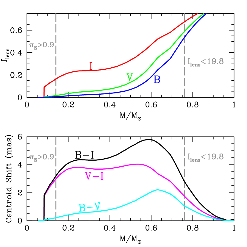
Figure 5: The top panel shows the fraction of the source$+$lens flux that is predicted to come from the lens in the I (F814W), V (F555W), and B (F435W) passbands as a function of lens mass. The bottom panel shows the predicted color-dependent centroid shifts as a function of mass for 2.4 years of relative proper motion at $\mu_{\rm rel}=8.4\,$mas/yr. The grey dashed lines indicate the upper and lower limits on the lens mass due to the upper limits on the microlensing parallax and lens brightness.

Figure 4(d) shows the probability distribution of the $I$-band magnitude of the planetary host star compared to the source star at $I=20.58\pm 0.10$. The implied planetary host star brightness distribution has a median and 1-$\sigma$ range of $I_{\rm lens}=21.9{+0.7\atop-1.1}$, but the most interesting feature of this figure is that the probability of a main sequence lens fainter than $I=23$ vanishes. This is because the mass-distance relation, eq. 1 ensures that the lens star will be nearby and at least at bright as $I=23$, even if it is at the bottom of the main sequence at $M_{\ast}=0.08M_{\odot}$. In fact, the microlensing parallax constraint from the light curve yields a lower limit for the lens star mass of $M_{\ast}\lower 2.15277pt\hbox{$\;\buildrel>\over{\sim}\;$}0.14M_{\odot}$. Thus, as the upper panel of Figure 5 indicates, the planetary host star must be at least 16% of the brightness of the combined lens plus source star blended image, and this implies that it will be detectable if it is not a stellar remnant. So, for the faintest possible main sequence lens star of the minimum mass, $M_{\ast}=0.14M_{\odot}$, eq. 5 implies that $f_{L}$ can be determined with a precision of 0.017 in a single orbit of HST ACS/HRC observations in the F814W pass band (with 97,000 detected photons). This allows a tight constraint on a bright binary companion to the source star. The situation is a bit worse for $f_{L}\sim 0.5$ when the source and lens are almost equally bright, but in this case, Figure 5 shows that the lens star will be easily detectable in the $V$ and $B$ passbands, where the HST PSF ($s_{0}$) is considerably sharper. So, we don’t anticipate a significant problem in measuring $f_{L}$, as long as we have a measurement of $F_{S}$ in more than one passband.

If we assume the most likely case of no detectable companion to the source, then eq. 4 implies that $\mu_{\rm rel}$ can be measured with a precision of 4.3% in a single orbit of HST ACS/HRC observations in the F814W pass band (with 97,000 detected photons). This is an improvement over the 7% measurement of $\mu_{\rm rel}$ that comes from the microlensing light curve, and would provide independent confirmation of the planetary interpretation of the light curve.

The color dependent effects visible in high resolution images of the OGLE-2005-BLG-169 lens and source star blend are summarized in Figure 5, which is based upon the measured relative lens-source proper motion for this event. The top panel shows the fraction $f_{L}$ of the source plus lens light that is contributed by the lens for different HST ACS/HRC passbands, and the bottom panel shows the predicted color dependent image center shifts. Both of these are shown as a function of the planetary host star mass, and the dashed grey lines indicate the constraints on the host star mass, $0.14M_{\odot}\leq M_{\ast}\leq 0.76M_{\odot}$, implied by the existing observational limits on the microlensing parallax effect and the maximum brightness of the lens star.

Several features are apparent in Figure 5. First, a measurement of a color dependent centroid shift does not yield a unique mass, because there are usually two different masses that yield the same centroid shift. This occurs because the centroid shift can become small if the lens star is faint or if the lens star has a similar color to the source star. However, this will generally not create an ambiguity in the interpretation of events because the brightness of the source star is known. The “faint lens” solution implies a fainter total brightness for the lens plus source blend than the “similar color” solution. Thus, the centroid shift degeneracy is broken by the constraint on the lens star brightness, which we get from the light curve. Also, if the system is observed in more than two passbands, the multiple color dependent centroid shifts will also resolve this degeneracy.

Figure 5 also indicates that it will be difficult to determine the OGLE-2005-BLG-169L lens star mass precisely if it is in the range $0.2M_{\odot}\lower 2.15277pt\hbox{$\;\buildrel<\over{\sim}\;$}M_{\ast}\lower 2.15277pt\hbox{$\;\buildrel<\over{\sim}\;$}0.4M_{\odot}$, because in this mass range the increase in the $I$-band lens brightness with distance due to the mass-distance relation (eq. 1) is nearly compensated for by the decrease in brightness due to the greater lens distance. This effect is also responsible for the peak at $I_{\rm lens}\simeq 21.9$ in Figure 4(d). This ambiguity can be resolved with observations in other passbands. The $V$ and $B$-band lens brightness fractions and the $B-V$ centroid shift curve does not have this ambiguity. However, the lens is also predicted to be rather faint in these bands if the lens mass is in the ambiguous range. So, it would be sensible to attack this question with a later set of observations if the lens star appears to lie in the $0.2M_{\odot}\lower 2.15277pt\hbox{$\;\buildrel<\over{\sim}\;$}M_{\ast}\lower 2.15277pt\hbox{$\;\buildrel<\over{\sim}\;$}0.4M_{\odot}$ mass range to take advantage of the larger lens-source separation at later times. Note that this near degeneracy does not occur for planetary host stars that reside in the Galactic bulge because the mass-distance relation becomes quite steep when $D_{L}$ approaches $D_{S}$.

4 Complete Lens Solutions from a Space-Based Microlensing Survey

While follow-up observations with HST or JWST may be feasible for a handful of planets discovered each year by microlensing, it will probably be difficult to obtain enough observing time to follow-up all the planets discovered by microlensing when the discovery rate increases. Certainly, with the expected discovery rate of many hundreds or even a thousand planets per year from a dedicated space mission (Bennett & Rhie, 2002), like the proposed Microlensing Planet Finder (MPF) (Bennett et al., 2004), it seems virtually certain that only a very small fraction of events could be followed up with observations with HST or JWST. Fortunately, a space-based microlensing survey will have the capability to perform its own follow-up observations.

The angular resolution of a dedicated space-based microlensing survey, like MPF, will be worse than HST’s resolution due to its smaller aperture (1.1m vs. 2.4m) and near-IR passband. However, the decreased angular resolution is more than compensated for by the much greater total exposure time that will be provided by a dedicated space telescope. While the MPF PSF may be three times the width of the HST PSF, but the number of detected photons in a 1-month MPF exposure can be a factor of 3000 times the number of photons detected in a single HST orbit. For fixed $f_{L}$, eq. 4 gives

$$\frac{\sigma_{\mu}}{\mu_{\rm rel}}\propto\frac{s_{0}^{2}}{\sqrt{2N_{tot}}\Delta x^{2}}\,$$ (11)

so we expect that MPF will be able to measure $\mu_{\rm rel}$ about 6 times more precisely than a single orbit HST observation (for fixed $\Delta x$).

A space-based survey, like MPF, will have several methods that can be used to obtain the complete solution of the microlensing event. These include:

1. Combining the mass-distance relation, eq. 1 with a main sequence mass-luminosity relation similar to those shown in Figure 1, as described in Section § 2.6, usually gives the most precise results. The angular Einstein radius, $\theta_{E}$ can be determined from the measurement of finite source effects in the light curve (i.e. by determining $t_{\ast}$), or by a measurement of the image elongation, as described in § 2.2.

2. The masses and distances can also be estimated from the brightness and color measurements of the lens light as seen by the space-based survey. This method is not generally as precise as method 1, but it can be considered to be an independent check on method 1. It can also constrain the possibility of a binary companion to the lens star that is too close or distant for its lensing effects to be apparent (Han, 2005), as discussed in § 2.5 and § 2.6.

3. The lens masses can be determined by combining measurements of $\mu_{\rm rel}$ and the microlensing parallax effect. This has the advantage that it can be used even when the lens star is too faint to detect, but a complete microlensing parallax measurement will only be available for events that are longer than average.

The two main methods for determining the lens-source relative proper motion, $\mu_{\rm rel}$, differ in that the measurement of the source radius crossing time, $t_{\ast}$, only determines the magnitude of $\mu_{\rm rel}$, while the measurement of the image elongation determines the full two dimensional vector, ${\mbox{\boldmath$\bf\mu$}_{\rm rel}}$. This is useful because it is generally much easier to measure only a single component (Gould, 1998) of the projected Einstein radius, ${\bf\tilde{r}_{e}}$, which is a two-dimensional vector with a length equal to the Einstein radius projected to the position of the Sun and a direction parallel to the transverse component of the lens-source relative velocity. However, since ${\bf\tilde{r}_{e}}\parallel{\mbox{\boldmath$\bf\mu$}_{\rm rel}}$, the measurement of a single component of ${\bf\tilde{r}_{e}}$ can be combined with the direction of ${\mbox{\boldmath$\bf\mu$}_{\rm rel}}$, to yield the magnitude of the projected Einstein radius, which is needed to determine the lens system masses via eq. 2.

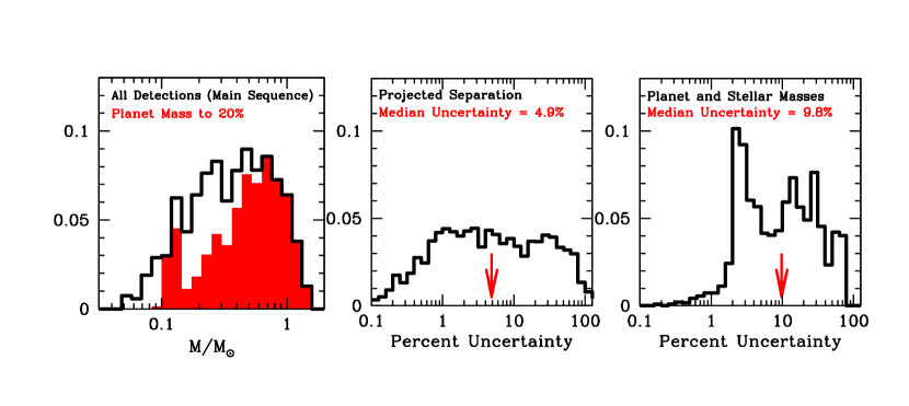
Figure 6: (a) The simulated distribution of stellar masses for stars with detected terrestrial planets. The red histogram indicates the subset of this distribution for which the masses can be determined to better than 20%. (b) The distribution of uncertainties in the projected star-planet separation. (c) The distribution of uncertainties in the star and planet masses. Note that it is the two-dimensional projected separation that is presented here, and we have not included the uncertainty in the separation along the line-of-sight as was done in Figure 4.

We have simulated (Bennett & Rhie, 2002) the planetary events expected for a space-based microlensing survey similar to the MPF mission (Bennett et al., 2004) to determine how well the parameter of the detected planetary systems can be determined. The results of these simulations are displayed in Figure 6. The parameters are solved for using methods 1 and 3 above, and the method that gives the most precise parameters is reported in Figure 6. One simplifying assumption that we have made is to assume that only the single component microlensing parallax asymmetry can be measured, instead of the full ${\bf\tilde{r}_{e}}$ vector. This means that we don’t have a direct method to determine the lens masses for planetary host stars that are too faint to detect. (These are generally white dwarfs, brown dwarfs, and late M-dwarfs). If we assume that planetary masses scale in proportion to the host star mass, but does not otherwise depend on stelar type, then about 24% of stars would fall into this “invisible star” category.

Figure 6 considers only planets found orbiting main sequence host stars, and panel (a) indicates that the distribution of host star masses is rather flat with precise mass determinations most common for the more massive host stars. Panels (b) and (c) show the distributions of the separation and mass uncertainties from these simulations with median uncertainties of 5.2% and 10.2%, respectively. These simulations clearly show that for the majority of planets discovered by a space-based microlensing survey, the star and planet masses, separation and host star type will be determined with reasonable precision.

5 Discussion and Conclusions

We have shown that the main uncertainties in the properties of planetary microlensing events can be overcome with space-based observations. For planets detected with ground-based microlensing observations, space-based follow-up imaging can detect the lens star, which allows the properties of the star and its planet to be determined. For a space-based microlensing survey, no follow-up observations are needed because the survey data will contain the information needed to identify the lens star and solve for the masses and separation.

The space-based observations in this paper apply primarily to events with main sequence source stars. Main sequence stars are the prime targets for space-based microlensing surveys (Bennett & Rhie, 2002) and for ground-based attempts to find earth-mass planets (Bennett & Rhie, 1996; Wambsganss, 1997). However, giant source stars do allow the detection of planets a bit more massive than the Earth, including the lowest mass planet detected to date, OGLE-2005-BLG-390Lb, (Beaulieu et al., 2006), around a main sequence star. (Of course, much lower mass planets have been discovered orbiting a pulsar (Wolszczan & Frail, 1992; Konacki & Wolszczan, 2003).)

While giant source stars are attractive targets for microlensing planet searches because their photometry is less affected by blending and because they require much shorter exposure times for precise photometry, they have the drawback that the source star is generally brighter than the lens star by a large factor. In eq. 4, if $F_{s}\gg F_{l}$, then $N_{tot}\propto F_{s}$ and $f_{L}\propto 1/F_{s}$, so $\sigma_{\mu}/\mu_{\rm rel}\propto 1/\sqrt{F_{s}}$. Thus, since typical red clump giant sources are brighter than the typical main sequence source stars by a factor of $\sim 100$, we expect that $\mu_{\rm rel}$ could be measured about ten times worse for a giant source than for the same event parameters with a main sequence source star. It would 100 times more exposure time to compensate for this, which seems implausible in all but the most favorable cases. A more reasonable strategy would be to wait longer to allow $\Delta x$ to grow, or to switch to an instrument with much higher angular resolution than HST, such as the Very Large Telescope Interferometer (VLTI) (Schöller et al., 2006). While current VLTI instrumentation is unable to observe the lens-source separation (Delplancke et al., 2001), it is expected that a future VLTI instrument will be capable of detecting the OGLE-2005-BLG-390L lens star sometime in the next decade (Beaulieu et al., in preparation). It is also possible that high resolution adaptive optics imaging could be used to make some of the measurements that we have described here for events with main sequence source stars. This would require either very precise knowledge of the AO imaging PSF, or a longer delay between the planetary event and the follow-up imaging to provide a larger lens-source separation.

Our investigation has been incomplete in that we have only considered a subset of the information that might come from analysis of the microlensing parallax effect. For a small subset of very long timescale events, it is likely that the lens system parameters can be characterized much more precisely than we have estimated here. It is also likely that many events with a parallax asymmetry measurement, but without a measurement of the two-dimensional ${\bf\tilde{r}_{e}}$ vector will be able to have their parameters measured determined due to future high precision measurements of ${\mbox{\boldmath$\bf\mu$}_{\rm rel}}\parallel{\bf\tilde{r}_{e}}$ with future high angular resolution instruments like the VLTI or the James Webb Space Telescope (Gardner et al., 2006) with the added benefit of a long time baseline.

This paper has focused on the situation in which signals of both the lens star and planet are detected, but it is also possible to detect planets that are so far from their parent star that the star does not yield a photometric microlensing signal (Di Stefano & Scalzo, 1999; Han et al., 2005). In such a situation, it may be difficult to distinguish the light curves of planets in very distant orbits from those of unbound planets that have been ejected from the planetary systems that they were born in. But in the former case, the planetary host star will often be detectable by the methods described in this paper. If these methods should fail to detect the host star, follow-up observations with the Space Interferometry Mission (SIM) will allow the host star to be discovered via its astrometric gravitational microlensing signal (Han, 2006), which will work even for dark host stars, such as white or brown dwarfs. However, SIM observations of main sequence source stars may be limited by the long exposure times required for sources fainter than $V=19$.

It is often said that microlensing planet discoveries cannot be followed up, but this is not completely true. While a repeat of the photometric planetary signal will not usually occur for another $\sim 10^{6}\,$years, we have shown that most planetary events provide a prediction of the lens-source relative proper motion, $\mu_{\rm rel}$, which can be confirmed with high angular resolution follow-up observations with HST. Furthermore, these follow-up observations also allow the complete solution of the microlensing event, which includes the conversion of the planetary mass ratio into physical masses for the planet and its host star, as well as the projected star-planet separation in physical units. Finally, we have also shown that a dedicated space-based microlensing survey, such as MPF, will collect the data necessary to extract these follow-up observations in its own photometric survey images. Thus, a space-based microlensing survey will provide full lens event solutions, with planet and star masses, their separation in physical units, and their distance from us, for most of the planets that are discovered.

References

- Afonso et al. (2000) Afonso, C., et al. 2000, ApJ, 532, 340
- Alcock et al. (1995) Alcock, C., et al. 1995, ApJ, 454, L125
- Alcock et al. (2000) Alcock, C., et al. 2000, ApJ, 541, 270
- Alcock et al. (2001a) Alcock, C., et al. 2001a, ApJ, 552, 259
- Alcock et al. (2001b) Alcock, C. et al., 2001b, Nature, 414, 617
- An et al. (2002) An, J., et al. 2002, ApJ, 572, 521
- Anderson & King (2000) Anderson, J. & King, I. R. 2000, PASP, 112, 1360
- Anderson & King (2004) Anderson, J. & King, I. R. 2004, Hubble Space Telescope Advanced Camera for Surveys Instrument Science Report 04-15
- Beaulieu et al. (2006) Beaulieu, J.-P., et al. 2006, Nature, 439, 437
- Bennett & Rhie (1996) Bennett, D.P. & Rhie, S.H. 1996, ApJ, 472, 660
- Bennett & Rhie (2002) Bennett, D. P. & Rhie, S. H., 2002, ApJ, 574, 985
- Bennett et al. (1996) Bennett, D. P., et al. 1996, Nuc. Phys. B Proc. Sup., 51, 152
- Bennett et al. (2002) Bennett, D. P., et al. 2002, ApJ, 579, 639
- Bennett et al. (2004) Bennett, D. P., et al. 2004, SPIE, 5487, 1453, (astro-ph/0409218)
- Bennett et al. (2006) Bennett, D. P., Anderson, J., Bond, I.A., Udalski, A., Gould, A. 2006, ApJ, 647, L171
- Bond et al. (2001) Bond, I., et al. 2001, MNRAS, 327, 868
- Bond et al. (2004) Bond, I.A., et al. 2004, ApJ, 606, L155
- Boss (2006a) Boss, A.P. 2006a, Boss, A. P. 2006, ApJ, 643, 501
- Boss (2006b) Boss, A.P. 2006b, ApJ, 644, L79
- Derue et al. (1999) Derue, F., et al. 1999, A&A, 351, 87
- Delplancke et al. (2001) Delplancke, F., Górski, K. M., & Richichi, A. 2001, A&A, 375, 701
- Di Stefano & Scalzo (1999) Di Stefano, R., & Scalzo, R. A. 1999, ApJ, 512, 564
- Drake, Cook, & Keller (2004) Drake, A. J., Cook, K. H., & Keller, S. C. 2004, ApJ, 607, L29
- Drilling & Landolt (2000) Drilling, J.S. & Landolt, A.U. 2000, “Allen’s Astrophysical Quantities”, Cox, A.N., ed., Springer-Verlag, New York, pp. 388-393
- Drimmel & Spergel (2001) Drimmel, R., & Spergel, D. N. 2001, ApJ, 556, 181
- Gardner et al. (2006) Gardner, J. P., et al. 2006, ArXiv Astrophysics e-prints, arXiv:astro-ph/0606175
- Gould (1992) Gould, A. 1992, ApJ, 392, 442
- Gould (1998) Gould, A. 1998, ApJ, 506, 253
- Gould, Bennett, & Alves (2004) Gould, A., Bennett, D. P., & Alves, D. R. 2004, ApJ, 614, 404
- Gould et al. (2006) Gould, A., et al. 2006, ApJ, 644, L37
- Gray (1992) Gray, D.F. 1992, “The Observation and Analysis of Stellar Photospheres”, Cambridge University Press, New York.
- Han (2005) Han, C. 2005, ApJ, 633, 414
- Han (2006) Han, C. 2006, ApJ, 644, 1232
- Han et al. (2005) Han, C., Gaudi, B. S., An, J. H., & Gould, A. 2005, ApJ, 618, 962
- Han & Gould (1995) Han, C. & Gould, A. 1995, ApJ, 447, 53
- Han et al. (2006) Han, C., Park, B., Kim, H., & Chang K., 2006, ApJ, submitted (astro-ph/0609095)
- Jaroszynski et al. (2005) Jaroszynski, M., et al. 2005, Acta Astronomica, 55, 159
- Kennedy et al. (2006) Kennedy, G. M., Kenyon, S. J., & Bromley, B. C. 2006, ApJ, 650, L139
- Ida & Lin (2004) Ida, S., & Lin, D.N.C. 2004, ApJ, 616, 567
- Konacki & Wolszczan (2003) Konacki, M., & Wolszczan, A. 2003, ApJ, 591, L147
- Kroupa & Tout (1997) Kroupa, P., & Tout, C.A. 1997, MNRAS, 287, 402
- Lada (2006) Lada, C. J. 2006, ApJ, 640, L63
- Lauer (1999) Lauer, T. R. 1999, PASP, 111, 1434
- Laughlin, Bodenheimer & Adams (2004) Laughlin, G., Bodenheimer, P., & Adams, F.C. 2004, ApJ, 612, L73
- Lovis et al. (2006) Lovis, C. et al. 2006, Nature, 441, 305
- Magain et al. (2006) Magain, P. et al. 2006, A&A, submitted, (arXiv:astro-ph/0609600)
- Mao & Paczyński (1991) Mao, S. & Paczyński , B. 1991, ApJ, 374, L37
- Mao (1999) Mao, S. 1999, A&A, 350, L19
- Poindexter et al. (2005) Poindexter, S., Afonso, C., Bennett, D. P., Glicenstein, J.-F., Gould, A., Szymański, M. K., & Udalski, A. 2005, ApJ, 633, 914
- Rivera et al. (2005) Rivera, E. J., et al. 2005, ApJ, 634, 625
- Schmidt-Kaler (1982) Schmidt-Kaler, T. 1982, in Landolt/Bornstein, Numerical Data and Functional Relationship in Science and Technology, New series, Group VI, Vol. 2b, p. 451
- Schöller et al. (2006) Schöller, M., et al. 2006, Proc. SPIE, 6268, 19
- Smith et al. (2002) Smith, M. C., Mao, S., & Woźniak, P. 2002, MNRAS, 332, 962
- Udalski et al. (2005) Udalski, A. et al. 2005, ApJ, 628, L109
- Wambsganss (1997) Wambsganss, T. R. 1997, MNRAS, 284, 172
- Wolszczan & Frail (1992) Wolszczan, A., & Frail, D. A. 1992, Nature, 355, 145