An Obliquely Propagating Electromagnetic Drift Instability in the Lower Hybrid Frequency Range

Abstract

By employing a local two-fluid theory, we investigate an obliquely propagating electromagnetic instability in the lower hybrid frequency range driven by cross-field current or relative drifts between electrons and ions. The theory self-consistently takes into account local cross-field current and accompanying pressure gradients. It is found that the instability is caused by reactive coupling between the backward propagating whistler (fast) waves in the moving electron frame and the forward propagating sound (slow) waves in the ion frame when the relative drifts are large. The unstable waves we consider propagate obliquely to the unperturbed magnetic field and have mixed polarization with significant electromagnetic components. A physical picture of the instability emerges in the limit of large wavenumber characteristic of the local approximation. The primary positive feedback mechanism is based on reinforcement of initial electron density perturbations by compression of electron fluid via induced Lorentz force. The resultant waves are qualitatively consistent with the measured electromagnetic fluctuations in reconnecting current sheet in a laboratory plasma.

JI, KULSRUD, FOX, AND YAMADA OBLIQUE ELECTROMAGNETIC DRIFT INSTABILITY Hantao Ji, Russell Kulsrud, and Masaaki Yamada, Center for Magnetic Self-organization in Laboratory and Astrophysical Plasmas, Plasma Physics Laboratory, Princeton University, Princeton, New Jersey 08543, USA. (hji@pppl.gov, rmk@pppl.gov, myamada@pppl.gov)

1 Introduction

Current-driven instabilities with frequencies higher than ion cyclotron frequency ($\omega>\Omega_{i}$) or wavelengths shorter than ion skin depth ($k\lambda_{i}>1;\lambda_{i}\equiv c/\omega_{pi}$) have been a popular subject for space and laboratory plasma research (see e.g. Gary, 1993). Recently, this topic has been revisited in the context of magnetic reconnection (see e.g. Biskamp, 2000), where intense current density exists locally in the diffusion region. In particular, the Lower Hybrid Drift Instability (Krall and Liewer, 1971) (LHDI) driven by a density gradient has received considerable attention as a potential source of anomalous resistivity.

When the LHDI propagates nearly perpendicular to the magnetic field it is purely electrotatic. Such waves have been observed at the low-$\beta$ edge of the current sheet in the laboratory (Carter et al., 2002a), in numerical simulations (see e.g. Scholer et al., 2003), and in space (Shinohara et al., 1998; Bale et al., 2002). They are driven unstable by inverse Landau damping of the drifting electrons.

However, these electrostatic modes are largely stabilized (Davidson et al., 1977) inside the high-$\beta$ reconnection layer, where the magnetic field gradient is large and the $\nabla B$ drift of the electrons is in the wrong direction to amplify the waves. Further, it is observed that their amplitudes do not correlate with the fast reconnection in the Magnetic Reconnection Experiment or MRX (Carter et al., 2002b). By contrast, magnetic fluctuations up to the lower hybrid frequency range have been more recently detected (Ji et al., 2004) in this high-$\beta$ center of the current sheet in the MRX. These propagate obliquely to the magnetic field, and their amplitudes exhibit positive correlations with fast reconnection. A theoretical explanation for the origin of these magnetic fluctuations, other than the electrostatic perpendicularly propagating LHDI waves, is therefore in order.

Earlier, motivated by observations of high frequency magnetic fluctuations in a magnetic shock experiment, Ross attempted (Ross, 1970) the first theoretical exploration of such candidate obliquely propagating electromagnetic high-frequency waves driven by a relative drift between electrons and ions associated with local currents. Based on a two-fluid formalism in the electron frame, Ross showed that unstable waves propagating obliquely to the magnetic field are excited by reactive coupling between ion beam and whistler waves. Such an instability is generally known as the Modified Two Stream Instability (McBride et al., 1972; Seiler et al., 1976) (MTSI) since it is driven by a local current across a magnetic field unrelated to a diagmagnetic drift.

Extensions to a full kinetic treatment of both ions and electrons were made for this instability (Lemons and Gary, 1977; Wu et al., 1983; Tsai et al., 1984). Unlike the perpendicular LHDI, the obliquely propagating MTSI persists in high-$\beta$ plasmas, where the critical values of relative drift for the instability are typically a few times the local Alfvén velocity, and possesses significant electromagnetic components. However, in most of these works, a finite pressure gradient self-consistent with the cross-field current was left out in the wave dynamics. This neglect throws doubt on the applicability of the MTSI to the MRX, where all the current is due to inhomogeneities.

Recently, global eigenmode analyses (Daughton, 1999; Yoon et al., 2002; Daughton, 2003) of the current driven instabilities have been carried out to take into account the effects of boundary conditions of a Harris current sheet (Harris, 1962). This followed earlier work on the same subject (Huba et al., 1980). It was found that for short wavelengths ($k\lambda_{e}\sim 1;\lambda_{e}\equiv c/\omega_{pe}$), the unstable modes concentrate at the low-$\beta$ edge, and they are predominantly electrostatic similar to the perpendicular propagating LHDI. In contrast, for relatively longer wavelengths ($k\sqrt{\lambda_{e}\lambda_{i}}\sim 1$), unstable modes with significant electromagnetic components develop in the center region. These are similar to the MTSI at high-$\beta$. For even longer wavelengths ($k\lambda_{i}\sim 1$), a drift kink instability (Daughton, 1999) is known to exist but this has a slower growth rate at more realistic ion-electron mass ratios. More recently, these analyses have been further extended to non-Harris current sheets (Yoon and Lui, 2004; Sitnov et al., 2004). When relative drift between electrons and ions is enhanced, the central region is clearly dominated by instabilities resembling the MTSI.

The first numerical simulations of the MTSI have been carried out in a two-dimensional local model (Winske et al., 1985), but focused on the electron heating. Particle simulations have also been carried out in three-dimensions to study stability of a Harris current sheet under various but limited conditions (Horiuchi and Sato, 1999; Lapenta and Brackbill, 2002; Daughton, 2003; Scholer et al., 2003; Shinohara and Fujimoto, 2004; Ricci et al., 2004). It was found that at first the LHDI like instabilities are active only at the low-$\beta$ edge, and modify the current profile which then leads to the long wavelength electromagnetic modes, such as drift kink instabilities or Kelvin-Helmholtz instabilities (Lapenta and Brackbill, 2002). Recent simulations using more realistic parameters (larger mass ratios with more particles) in larger dimensions indicate (Ricci et al., 2004) that the MTSI-like modes also develop in the central region. While the characteristics of the observed waves in the MRX current sheet are generally consistent with these linear stability analyses and nonlinear simulation results, there has been yet no convincing physical explanation of the observed electromagnetic waves in the lower hybrid frequency range. Comparisons between MTSI and LHDI, the latter of which involves a self-consistent pressure gradient, were made based on local kinetic theories (Hsia et al., 1979; Yoon et al., 1994; Silveira et al., 2002), but with a focus on nearly perpendicularly propagating waves. Extensions to larger propagation angles were also attempted earlier (Zhou et al., 1983; Zhou and Cao, 1991) but with few discussions on the underlying physics.

Motivated by the observations in the MRX and these recent theoretical developments, we investigate this instability based on a local two-fluid formalism in this paper. Our analysis is of the MRX and includes the self-consistent pressure gradient with large propagation angles. A local treatment is justified if the wavelength is short ($k\lambda_{i}\gg 1$) and the growth rate is large ($\gamma\gg\Omega_{i}$), compared to the global eigenmode analyses extending throughout the current layer (see for example Kulsrud (1967)). Our focus here is to reveal the underlying physics of the instability by using the simplest possible model rather than to carry out more involved calculations. We find that when the relative drifts are large, the instability is caused by a reactive coupling between the backward propagating whistler (fast) waves in the moving electron frame and the forward propagating sound (slow) waves in the ion frame. The unstable waves have a mixed electromagnetic character with both electrostatic and magnetic components. They propagate obliquely to the unperturbed magnetic field. The primary positive feedback mechanism for the instability is identified as reinforcement of initial electron density perturbations by an induced Lorentz force. The role this instability plays in magnetic reconnection, such as anomalous resistivity and heating, will be discussed in a forthcoming paper (Kulsrud et al., 2004) that is based on quasi-linear theory (see also Winske et al. (1985); Basu and Coppi (1992); Yoon and Lui (1993).)

2 Theoretical Model

The basic features of our model are described in this section. Since our main objective is to understand physics of the underlying instability, we develop a theoretical model, which contains the essential ingredients for the instability, yet remains simple enough so that the feedback mechanism can be understood. In contrast to the past work, most of which is based on full kinetic theory, we find that we are able to use a simple two-fluid theory and still obtain reliable results. We show that most features of the instability can be revealed by this simple model.

2.1 Method of the calculation

We wish to treat the LHDI mode by an approach somewhat different from earlier approaches. Our basic assumption is that the drift velocity is produced by equilibrium gradients (LHDI) rather than an ion beam (MTSI). In the MRX the gradients are the origin of the relative drift velocity of the ions and electrons which is just the diamagnetic currents, so that the instability is an LHDI. However, since the LHDI has been usually treated as a nearly perpendicular propagating mode and we restrict ourselves in this paper to propagation at angles finitely different from $90$ degrees, we refer to our instability as the obliquely propagating LHDI or more briefly the oblique LHDI.

The reason we do not consider the LHDI near 90 degrees is that it has been shown to be stable in the central regions of the MRX and, as discussed in the introduction, we are interested in explaining the observed instabilities there. In fact, as shown by Carter et al. (2002b), the gradient of the magnetic field is large there and the $\nabla B$ drifts cause the resonant electrons to drift in the opposite direction than inferred from their current. The oblique instability we investigate is a non resonant one.

We assume that the mode is at a large frequency compared to the ion cyclotron frequency, and the wave length is small compared to the ion gyration radius, so that the ions may be considered to be unmagnetized. We also assume that the frequency is small compared to the electron cyclotron frequency, $\Omega_{e}$, and that the wave length is large compared to the electron gyration radius, $\rho_{e}$, so that the electron can be treated by the drift kinetic theory. This theory is described in Appendix A1, but the upshot of it is that one expands the Vlasov equation in the small parameter $\rho_{e}/\lambda$ where $\lambda$ is the perpendicular scale of the perturbation as well as the equilibrium. One solves the Vlasov equation to lowest order to obtain the zero order electron distribution function $f_{0}$ from which one can obtain the electron pressure tensor, ${\bf P}_{e}$. Then one calculates the perpendicular velocity moment of the first order distribution function $f_{1}$, to find the perpendicular electron current. But this calculation is equivalent to taking the perpendicular electron fluid equation of motion with this pressure tensor. The parallel current is then obtained from the continuity equation, $\nabla\cdot{\bf j}^{e}-\partial(n_{e1}e)/\partial t=0$.

This procedure is totally equivalent to previous calculations giving identical results in the small $\rho_{e}$ limit. It might be argued that one should consider waves with $k_{\perp}\rho_{e}\sim 1$ since in previous work on the perpendicular LHDI the maximum growth occurs when $k_{\perp}\rho_{e}\sim 1$. However, for the oblique LHDI the maximum growth actually occurs when $k_{\perp}\rho_{e}\ll 1$ and the mode becomes stable for $k_{\perp}\rho_{e}$ that approaches unity. (The guiding center treatment is appropriate for inhomogeneous systems, since it makes no assumption about near homogeneity and avoids the complicating approximations concerning it that are usually made.)

It turns out that it is not appropriate to treat the pressure tensor as anisotropic for the MRX experiments, in which the magnetic fluctuations are observed. This is because the electron-ion collision rate is comparable to the frequencies and growth rates of the mode, so it is just as accurate to take the pressure as isotropic. Further, it is also appropriate to assume that the plasma is isothermal, so that $p=nT$ in general; $p_{0}=n_{0}(x)T$ in the equilibrium and $p_{1}=n_{1}T$ is the perturbation. The fact that $T$ is constant in the equilibrium over the region occupied by the mode is supported directly from observations. The fact that perturbations in the temperature are zero follows from the very large thermal conductivity along the lines, so that the thermal relaxation time is shorter than the perturbation growth time. With this assumption we can avoid the solution for $f_{0}$ and work entirely from the electron fluid equation, to determine the perpendicular electron currents.

At this point we are in a position to solve for the ion and electron currents in terms of the electric fields. However, one further physical result, charge neutrality, allows us to further shorten the calculation. Since the Debye length is very small compared to even the electron gyration radius, we may assume to an excellent approximation that the perturbed electron density $n_{e1}$ is equal to the perturbed ion density $n_{i1}$ and this enable us to easily evaluate the relevant terms in the perturbed equation of motions of the electrons. (Of course if we had avoided this step and solved directly for the ion and electron currents separately and then substituted in Maxwell’s equations, charge neutrality would have followed automatically. Introducing charge neutrality earlier leads to considerable simplicity in the calculation and more physical insight.)

To summarize our calculation: we first write down the equilibrium conditions. Then next we calculate the perturbed ion current and density from the unmagnetized ion dynamics. We then calculate the perturbed perpendicular electron current from the perpendicular equation of motion for the electrons. We can then find the parallel electron current from $\nabla\cdot{\bf j}=\nabla\cdot({\bf j}^{i}+{\bf j}^{e})=0$. Knowing these currents, we then substitute them into Maxwell’s equations to find three independent relations for the wave electric fields. However, it turns out that one of the three Maxwell’s equations can be simplified to the electron force balance along the field line. Thus, this eliminates the needs to calculate the parallel electron current directly from $\nabla\cdot{\bf j}=0$, which is demanded by the charge neutrality condition.

2.2 Equilibrium

For definiteness, we assume the MRX equilibrium is a Harris equilibrium and study it in the ion frame. This seems the most physical frame in which to study the instability since it turns out to be essentially an unstable sound mode which is carreid by the ions. We concentrate our attention on a small region say about half way out from the center of the Harris sheet.

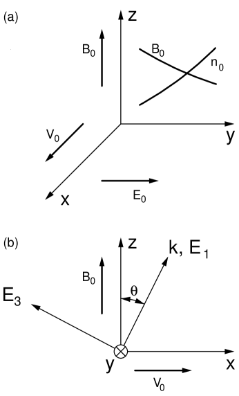
Figure 1: (a) Illustrations of the equilibrium state. Ions are at rest while electrons drift toward positive $x$ direction, crossing magnetic field in the $z$ direction. The resultant Lorentz force and electric field is balanced by pressure gradients in the $y$ direction, which points towards the current sheet center. (b) Definitions of $E_{1}$ and $E_{3}$. $E_{2}$ is same as $E_{y}$.

In this frame as shown in Fig.1(a), there is an electric field $E_{0}$ balancing their pressure force, $T_{i}\partial n_{0}/\partial y$, in the $y$ direction:

$$en_{0}E_{0}=T_{i}{\partial n_{0}\over\partial y}.$$ (1)

The magnetic field, $B_{0}$, is chosen in the $z$ direction. A current is carried by electrons drifting in the $x$ direction with a speed $V_{0}$. Force balance of the electron fluid then is given by

$$-en_{0}(E_{0}-V_{0}B_{0})=T_{e}{\partial n_{0}\over\partial y}$$ (2)

Eliminating ${\partial n_{0}/\partial y}$ in Eqs.(1,2), we have

$$E_{0}={T_{i}\over T_{e}+T_{i}}V_{0}B_{0}.$$ (3)

If the plasma resistivity is finite, the electron current in the $x$ direction cannot be maintained without an electric field in the same direction, $E_{x0}$. We shall see later, however, that its effects on the wave dynamics are small as in the MRX.

3 Dispersion Relation

All wave quantities are assumed to have a normal mode decomposition proportional to

$$\exp[i({\bf k}\cdot{\bf x}-\omega t)]$$

with the wave vector ${\bf k}=(k_{x},0,k_{z})$ and the wave angular frequency $\omega$. Note that ${\bf k}$ here does not have a $y$ component. This assumption is justified in a local theory if wavelengths are much smaller than the current layer thickness in the $y$ direction.

The governing equation between $\omega$ and ${\bf k}$, or the dispersion relation, follows from three independent equations that relate the three components of the wave electric field, $E_{x}$, $E_{y}$, and $E_{z}$. These can be derived from Ampere’s law and Faraday’s law,

$${\bf k}\times({\bf k}\times{\bf E})=-i\omega\mu_{0}{\bf j},$$ (4)

which leads to

$$k_{z}^{2}E_{x}-k_{x}k_{z}E_{z} = i\omega\mu_{0}j_{x}$$ (5)

$$k^{2}E_{y} = i\omega\mu_{0}j_{y}$$ (6)

$$k_{x}^{2}E_{z}-k_{x}k_{z}E_{x} = i\omega\mu_{0}j_{z}.$$ (7)

Here $\mu_{0}$ is the vacuum magnetic permeability. Next, we separately consider ion and electron dynamics to express the above equations in terms of the electric field.

3.1 Ion Dynamics

We take the ions as unmagnetized and solve the kinetic equation for the perturbed distribution function assuming the equilibrium ion distribution function is Maxwellian with constant temperature, but variable density, $dn_{0}/dy=\epsilon n_{0}$. From Eq.(1), $\epsilon=eE_{0}/T_{i}=2eE_{0}/Mv_{i}^{2}$.

The solution of the ion Vlasov equation is carried out as an expansion to first order in $\epsilon$. The result is most easily expressed in terms of the electric field components $E_{1}$ and $E_{3}$ defined in Fig.1(b), in which $E_{1}$ is the component parallel to ${\bf k}$, and $E_{3}$ is the component perpendicular to it and in the $x-z$ plane. The perturbed ion current can then be written (Appendix B1),

$${\bf j}^{i}=-i\frac{n_{0}e^{2}}{M}\frac{1}{kv_{i}}\left[Z(\zeta){\bf E}\right. - (\zeta Z^{\prime}+Z)({\bf E}\cdot\hat{{\bf k}})\hat{{\bf k}}$$ (8)

$$- \left.i(\epsilon/k)(\zeta Z^{\prime}+Z)E_{y}\hat{{\bf k}}\right]$$

and the perturbed ion density is

$$n=i\frac{n_{0}e}{Mk^{2}v_{i}^{2}}Z^{\prime}(\zeta)\left({\bf k}\cdot{\bf E}+i\epsilon E_{y}\right)$$ (9)

where $\hat{{\bf k}}={\bf k}/k$, $\zeta=\omega/kv_{i}$, and $Z$ is the plasma dispersion function. We find that for the principal instabilities the phase velocity is somewhat larger than $v_{i}$ so for convenience we first take the $\zeta\gg 1$ limit (the cold limit), determine the parameter range of instability. Then, in Appendix B3, we are able to employ a simple modification of the dispersion relation to extract the correct growth rate including the finite ion thermal effects.

In the cold limit the ion current neglecting the $\epsilon$ correction is obtained from the $\zeta\gg 1$ limit and is

$${\bf j}^{i}\approx i{\omega_{pi}^{2}\over\omega}\epsilon_{0}{\bf E},$$ (10)

where the ion plasma angular frequency $\omega_{pi}\equiv\sqrt{n_{0}e^{2}/M\epsilon_{0}}$ and $\epsilon_{0}$ is the vacuum susceptibility. In the same limit the perturbed ion density is

$$n=i\frac{n_{0}e}{M\omega^{2}}({\bf k}\cdot{\bf E}+i\epsilon E_{y})\approx i{en_{0}\over M\omega^{2}}({\bf k}\cdot{\bf E}).$$ (11)

The neglected $\epsilon$ term is much smaller than the other one since, for our local theory, we assume $k/\epsilon\gg 1$. Indeed, it is shown in Appendix B2 that the neglected term only has a small effect on the dispersion relation.

3.2 Electron Dynamics

As we have shown in Appendix A1, the perpendicular electron current can be obtained from the first order force balance for the electron fluid,

$${\bf j}^{e}\times{\bf B}_{0}=en_{0}{\bf V}_{0}\times{\bf B}+en_{0}{\bf E}+en{\bf E}_{0}+T_{e}\nabla n+mn_{0}{\partial{\bf U}_{E}\over\partial t}$$ (12)

where ${\bf U}_{E}={\bf E}\times{\bf B_{0}}/B_{0}^{2}$ and $m$ is the electron mass. As shown in Appendix A2, the electron inertial terms contribute a small effect to the distpersion relation and we can neglect them when determining the instability. The $y$ and $x$ components of Eq.(12), therefore, are given by

$$-j_{x}^{e}B_{0} = -en_{0}V_{0}B_{z}+en_{0}E_{y}+enE_{0}$$ (13)

$$j_{y}^{e}B_{0} = en_{0}E_{x}+ik_{x}T_{e}n$$ (14)

respectively. Here, $B_{z}=k_{x}E_{y}/\omega$. Since $E_{0}$ and $n$ are given already by Eq.(3) and Eq.(11), $j_{x}^{e}$ and $j_{y}^{e}$ can be expressed in terms of the electric field.

We note on the righthand side of Eq.(14) that there would be another term, $enE_{x0}$, where $E_{x0}$ is the unperturbed electric field. However, we will treat it as second order and balanced by quasi-linear terms (Kulsrud et al., 2004). In fact, the contribution from this term is small when compared with the last term if $k_{x}\gg eE_{x0}/T_{e}$ as is often satisfied in the MRX.

The $z$-component of the electron current, $j_{z}^{e}$, is not determined by Eq.(12). It turns out, however, that it is unnecessary to explicitly calculate it in order to obtain the dispersion relation due to simplifications of the $z$-component of Maxwell’s equation, Eq.(7). This is because the electrons are so easily accelerated along the field line by the force, $F_{z}^{e}$, on the electron fluid where

$$F_{z}^{e}=-n_{0}e\left(E_{z}+V_{0}B_{x}+ik_{z}{T_{e}\over e}{n\over n_{0}}\right).$$

The various terms in this force are separately large and must balance closely to avoid very large parallel electrons currents. In fact, taking $j_{z}^{e}=-n_{0}ev_{z}^{e}=-i(e/m\omega)F_{z}^{e}$ and using Eq.(10) for the ion current, we can write the $z$-component of Maxwell’s equation, Eq.(7), as

$$k_{x}^{2}E_{z}-k_{x}k_{z}E_{x}=i\omega\mu_{0}(j_{z}^{i}+j_{z}^{e})$$

$$=-{\omega_{pi}^{2}\over c^{2}}E_{z}-{\omega_{pe}^{2}\over c^{2}}\left(E_{z}+V_{0}B_{x}+ik_{z}{T_{e}\over e}{n\over n_{0}}\right).$$ (15)

Since $\omega_{pi}^{2}/\omega_{pe}^{2}=m/M\ll 1$ and $(k\lambda_{e})^{2}\ll 1$ to our interests here, the above equation simplifies to the one demanding the electron force balance in the $z$ direction,

$$E_{z}+V_{0}B_{y}+ik_{z}{T_{e}\over e}{n\over n_{0}}=0,$$ (16)

where $B_{y}$ can be expressed in terms of the electric field using Faraday’s law,

$$B_{y}={k_{z}E_{x}-k_{x}E_{z}\over\omega}.$$

In Appendix A2, we show that the neglected terms have only a small effect on the dispersion relation. We note that, although unneeded for the dispersion relation, the $z$-component of the electron current, $j_{z}^{e}$, can be determined by $\nabla\cdot{\bf j}=0$. This is a consequence of the charge-neutrality condition, which is in turn enforced by Eq.(16).

It is interesting to note that if we allow the propagation angle approach to $90^{\circ}$, the parallel phase velocity can be comparable to the electron thermal velocity. In this case, we need to include a Landau term in Eq.(16). Then, if $\beta_{e}\ll 1$, we would be able to recover the electrostatic perpendicular LHDI (Krall and Liewer, 1971). However, since this electrostatic LHDI disappears at the high-$\beta$ of interest to us, we need not include the Landau term.

3.3 Dispersion Relation

Substituting expressions of ${\bf j}^{e}$, ${\bf j}^{i}$, and $n$ [Eqs.(10,13,14,11)] into Eqs.(5,6,16) we obtain, after some algebra, the dispersion relation

$$\left(\begin{array}[]{ccc}D_{xx}&D_{xy}&D_{xz}\\ D_{yx}&D_{yy}&D_{yz}\\ D_{zx}&D_{yz}&D_{zz}\end{array}\right)\left(\begin{array}[]{c}E_{x}\\ E_{y}\\ E_{z}\end{array}\right)=0,$$ (17)

where

$$D_{xx}= K^{2}\cos^{2}\theta+1-\displaystyle{\beta_{i}\over\beta_{e}+\beta_{i}}{KV\sin\theta\over\Omega}$$

$$D_{xy}= i(\Omega-KV\sin\theta)$$

$$D_{xz}= -K^{2}\sin\theta\cos\theta-\displaystyle{\beta_{i}\over\beta_{e}+\beta_{i}}\displaystyle{KV\cos\theta\over\Omega}$$

$$D_{yx}= -i\left(\Omega-\displaystyle{\beta_{e}\over 2}\displaystyle{K^{2}\sin^{2}\theta\over\Omega}\right)$$

$$D_{yy}= K^{2}+1$$

$$D_{yz}= i\displaystyle{\beta_{e}\over 2}\displaystyle{K^{2}\sin\theta\cos\theta\over\Omega}$$

$$D_{zx}= KV\cos\theta-\displaystyle{\beta_{e}\over 2}\displaystyle{K^{2}\sin\theta\cos\theta\over\Omega}$$

$$D_{zy}= 0$$

$$D_{zz}= \Omega-KV\sin\theta-\displaystyle{\beta_{e}\over 2}\displaystyle{K^{2}\cos^{2}\theta\over\Omega}.$$

Here the dimensionless parameters are defined by Ω≡ωωci,     K ≡kcωpi,     V ≡V_0 VA,     β_e ≡n_0 T_e B02/2μ0,
β_i ≡n_0 T_i B02/2μ0,     sinθ≡k_x k. Here, $\omega_{ci}$ is the ion cyclotron angular frequency $eB_{0}/M$ and $V_{A}$ the Alfv́en speed $B_{0}/\sqrt{\mu_{0}Mn_{0}}$.

The $KV$ term in $D_{{xx}}$ and in $D_{xz}$ and the $\beta_{e}$ terms all result from replacing the kinetic equation for the perturbed density $n$ by it cold limit. The ’one’s in $D_{xx}$ and $D_{yy}$ are ion currents which are similarly appoximated.

The resultant dispersion relation $\Omega(K)$ is a fourth order algebraic equation in $\Omega$ with 4 controlling parameters, $V$, $\beta_{e}$, $\beta_{i}$, and $\theta$, Ω^4 -2KVsinθΩ^3
-[(K^2+1)(K^2cos^2θ+1) -K^2V^2sin^2θ+β_e2K^2]Ω^2
+KVsinθ[β_eK^2+(K^2+1)β_e+2β_i βe+βi] Ω
+K^2[ β_e2[ (K^2+1)^2cos^2θ-K^2V^2sin^2θ]
-(K^2+1)V^2β_i βe+βi]=0.

4 Wave Characteristics and Instability

4.1 Basic Wave Characteristics without Drift

The basic wave characteristics described by Eq.(3.3) are summarized here for the case that there is no drift between ions and electrons. When $V=0$ and $\theta=0$, Eq.(3.3) reduces to

$$\left[\Omega^{2}-(K^{2}+1)^{2}\right]\left[\Omega^{2}-{\beta_{e}\over 2}K^{2}\right]=0$$

which represents four waves, as shown in Fig.2 for the case of $\beta_{e}=\beta_{i}=1$. Two waves are whistler waves, traditionally termed fast waves, while the other two waves are sound waves or slow waves. One of each waves propagates along the background magnetic field and the other propagates against. As expected, the whistler waves are largely transverse waves or electromagnetic waves since the electric field vectors are perpendicular to the propagation (${\bf k}$) direction $\phi\simeq 90^{\circ}$, where $\cos\phi\equiv{\bf k}\cdot{\bf E}/(|{\bf k}||{\bf E}|)$. In contrast, the sound waves are largely longitudinal waves or electrostatic waves since $\phi\simeq 0$.

The situation changes when $\theta$ and $\beta$ are varied. In Fig.3, the angles between ${\bf E}$ and ${\bf k}$, $\phi$, are shown for $V=0$ and a few cases of $\theta$ and $\beta$. It can be seen that when $\theta$ is larger, the whistler waves become less electromagnetic and more electrostatic while the sound waves become more electromagnetic and less electrostatic. This trend is stronger for larger values of $\beta$.

4.2 An Oblique Electromagnetic Instability

It is evident that the whistler waves are supported by fast electron dynamics while the sound waves are supported by slow ion dynamics. When there is no drift between these two fluids, all wave branches stay separate in the dispersion diagram as shown in Fig.2 for $\theta=0$. The situation is similar for more general cases of $\theta\neq 0$. If $V=0$, Eq.(3.3) reduces to Ω^4 - [(K^2+1)(K^2cos^2θ+1)+β_e2K^2] Ω^2
+β_e2K^2(K^2+1)^2cos^2θ=0, which represents four waves in the left panels in Fig.4 for the case of $\theta=60^{\circ}$ and $\beta_{e}=\beta_{i}=1$. It is seen that at this propagation angle, $\phi$ is $\sim 40^{\circ}$ for whistler waves and $\sim 0^{\circ}$ for sound waves.

When there is a finite electron drift in the ion rest frame, the whistler waves are doppler-shifted so that each $\Omega$ from Eq.(4.2) is increased by $KV\sin\theta$, shown as dotted curves in the top-right panel of Fig.4 for the case of $V=6$. In constrast, sound waves, unaffected by the drift, are shown as dotted straight lines. When the drift is large, some part of the backward propagating whistler waves branch can intercept with the forward propagating sound wave branch, resulting in instabilities through reactive couplings. The case of $V=6$ is shown in the right panels of Fig.4 and all other parameters are the same as in the left panels. It is seen that when $K<\sim 6$ or $K>\sim 16$, all four roots are real and thus all waves are stable. When $6<K<16$, two of roots become complex conjugates as a result of coupling; one of them is damped and another growing (the growth rates are shown in the middle-right panel). The maximum growth rate is about 8 times of $\omega_{ci}$ at $K\simeq 11$. Since the polarization angle $\phi\simeq 15^{\circ}$, the unstable waves have significant electromagnetic components.

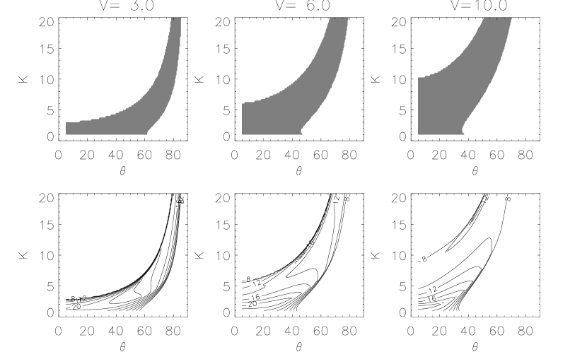
Figure 5: Unstable region where Im$(\Omega)>0$ (filled regions in top panels) and contours of polarization angle ($\phi$, bottom panels) in the $\theta-K$ plane for the cases of $V=3,6,10$ and $\beta_{e}=\beta_{i}=1$.

Figure 5 shows the unstable region and contours of polarization angle in the $\theta-K$ plane for a few values of $V$. It is seen that the unstable waves are localized to small $K$ when $\theta$ is small and to large $K$ when $\theta$ is large. The unstable region expands and the growth rate increases with increasing $V$. The polarization angle $\phi$ ranges between $10^{\circ}$ to $25^{\circ}$, and is larger near the small $K$ and small $\theta$ corner.

5 A Physical Picture

5.1 Further Simplification of Electron Dynamics

In order to understand the primary feedback mechanism of our instability we make further simplifications to the dispersion relation given by Eq.(17). We first start by rotating the coordinate for ${\bf E}$ as shown in Fig.1(b): $(E_{x},E_{y},E_{z})$ to $(E_{1},E_{2},E_{3})$. $E_{1}$ is in the $k$ direction, representing the electrostatic component. $E_{2}$ is the same as $E_{y}$ and $E_{3}$ is another perpendicular component to ${\bf k}$, and both of these are electromagnetic components. Using the new bases, $(E_{1},E_{2},E_{3})$, Eq.(17) reduces to

$$\left(\begin{array}[]{ccc}D_{11}&D_{12}&D_{13}\\ D_{21}&D_{22}&D_{23}\\ D_{31}&D_{32}&D_{33}\end{array}\right)\left(\begin{array}[]{c}E_{1}\\ E_{2}\\ E_{3}\end{array}\right)=0,$$ (18)

where

$$D_{11}= \sin\theta-\displaystyle{\beta_{i}\over\beta_{e}+\beta_{i}}{KV\over\Omega}$$

$$D_{12}= i(\Omega-KV\sin\theta)$$

$$D_{13}= -(K^{2}+1)\cos\theta$$

$$D_{21}= -i\displaystyle{\sin\theta\over\Omega}\left(\Omega^{2}-\displaystyle{\beta_{e}\over 2}K^{2}\right)$$

$$D_{22}= K^{2}+1$$

$$D_{23}= i\Omega\cos\theta$$

$$D_{31}= \displaystyle{\cos\theta\over\Omega}\left(\Omega^{2}-\displaystyle{\beta_{e}\over 2}K^{2}\right)$$

$$D_{32}= 0$$

$$D_{33}= \Omega\sin\theta-KV.$$

Again the $KV$ term in $D_{11}$ and the $\beta_{e}$ terms result form approximating the perturbed density, and the ’one’s in $D_{13}$ and $D_{22}$ from approximating the ion currents.

Next we simplify these equations by taking the limit of large $\Omega$, $K$, and $V$ since this asymptotic limit will make the physical mechanism of the instability clear. The simplified matrix then reduces to

$$\left(\begin{array}[]{ccc}-\displaystyle{{\beta_{i}\over\beta_{e}+\beta_{i}}{KV\over\Omega}}&-iKV\sin\theta&-K^{2}\cos\theta\\ -i\displaystyle{\sin\theta\over\Omega}\left(\Omega^{2}-\displaystyle{\beta_{e}\over 2}K^{2}\right)&K^{2}&0\\ \displaystyle{\cos\theta\over\Omega}\left(\Omega^{2}-\displaystyle{\beta_{e}\over 2}K^{2}\right)&0&-KV\end{array}\right).$$ (19)

Each line of the above matrix equation represents the balance of the leading forces on the electron fluid along the three coordinate directions $y,x,z,$ respectively. By referring back to Eq.(7) and Eq.(12) we can see that the force balance can be written

$$\begin{array}[]{ccc}y:&-enE_{0}-j_{0x}B_{z}-j_{x}B_{0}=0\\ x:&-en_{0}E_{1}\sin\theta-\partial p_{e}/\partial x+j_{y}B_{0}=0\\ z:&-en_{0}E_{1}\cos\theta-\partial p_{e}/\partial z+j_{0x}B_{y}=0\end{array},$$ (20)

where in the asymptotic limit the current ${\bf j}$ is all due to the electrons. Interestingly, the electrostatic force is balanced by the Lorentz force in all directions. In the $y$-direction, the unperturbed electrostatic field acting on the perturbed electron density is balanced by the Lorentz force, which consists of both magnetic pressure gradient, $-j_{0x}B_{z}$, and tension $-j_{x}B_{0}$ forces. By contrast, the perturbed electrostatic field is balanced by the magnetic tension, $j_{0x}B_{y}$, in the $z$-direction.

5.2 The Case of $\theta$=0

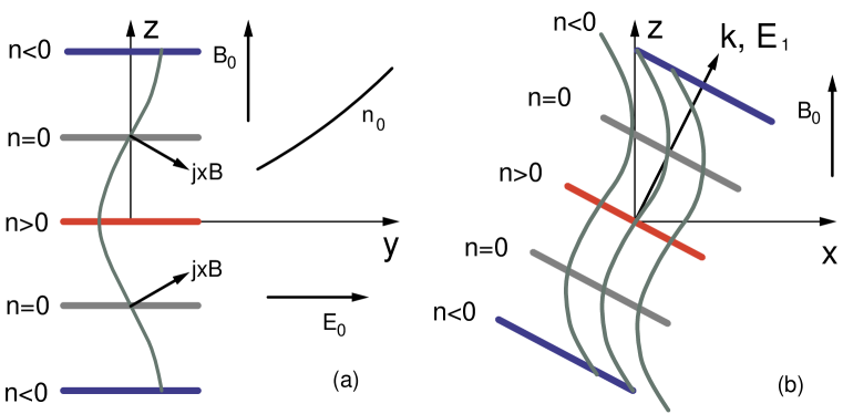
Figure 6: Illustrations of the instability mechanism (a) when $\theta=0$ in the $y-z$ plane and (b) when $\theta>0$ in the $x-z$ plane. This distance between the field lines indicates the relative field strength.

We start with the simplest case, $\theta=0$, in which there are no perturbed forces in the $x$-direction. In the $y$-direction the perturbed magnetic pressure force is also zero since $B_{z}=k_{x}E_{y}/\omega=0$. Therefore, the electrostatic force, $-enE_{0}$, must be balanced by the magnetic tension force, $-j_{x}B_{0}$. Suppose that the electron density is perturbed in a way such that $n>0$ at the origin as illustrated in Fig.6(a) in the $y-z$ plane. Because ${\bf E}_{0}$ points in the positive $y$-direction, the perturbed electrostatic force on the electron fluid, $-enE_{0}$, points in the negative $y$-direction at the origin. Since it varies in $z$, this force bends the field line until its magnetic tension force $-j_{x}B_{0}$ balances the $-enE_{0}$ force. (Here the field-line bending can also be understood as a result of the perturbed $j_{x}$ due to changing the number of the charged carriers by the perturbed density $n$.)

In the $z$-direction, there is now a component of the magnetic tension force towards the origin $j_{0x}B_{y}$ due to the bent line, as illustrated in Fig.6(a). This force reduces or reverses the perturbed electrostatic force $-en_{0}E_{1}$ produced by the electron density perturbation. In the latter case, the perturbed electrostatic force is directed away from the regions where $n>0$ and towards the regions where $n<0$. As a result the perturbed electric field, ${\bf E}_{1}$, must point from the regions where $n<0$ to the regions where $n>0$, such as the origin.

To see that this leads to instability consider the ions which only see the electrostatic field ${\bf E}_{1}$. This electrostatic field will force the ions to condense further at the origin increasing their density perturbation. By charge neutrality this will increase the initially assumed electron density perturbation and thus lead to instability.

5.3 The Case of $\theta>0$

We find that it is convenient to take the limit of $\beta_{e}=0$ for the discussion of this more general and complicated case. Here the feedback to initial perturbations through compression or decompression of the electron fluid along the $z$-direction is unaffected except for a reduced efficiency. However, there are perturbed forces in the $x$-direction. As before, we suppose an electron density perturbation $n>0$ at the origin. When the mode is unstable, the perturbed electrostatic force, which is parallel to ${\bf k}$, has an $x$-component, $-en_{0}E_{1}\sin\theta$, pointing away from the regions where $n>0$ towards the regions where $n<0$ also as before. This force on the electrons decompresses the magnetic field in the $n>0$ regions and compresses it in the $n<0$ regions. This is illustrated in Fig.6(b) in the $x-z$ plane. Because ${\bf k}$ makes a finite angle to ${\bf B}_{0}$, the magnetic field lines are distorted to have both a tension force and also a magnetic pressure force. Therefore, $B_{z}$ must be negative (decompressed) at the origin where $n>0$ and thus, the associated magnetic pressure force in the $y$-direction, $-j_{0x}B_{z}$, is directed towards positive $y$-direction. As a result, this force counters the initial electrostatic force, $-enE_{0}$, (which bends the field line) and thus, reduces the tendency towards instability.

Both these stabilizing and destabilizing forces are included in the dispersion relation from Eq.(19), in which we restore $\beta_{e}$ to obtain

$$\Omega^{2}={\beta_{e}\over 2}K^{2}+{\beta_{i}\over\beta_{e}+\beta_{i}}{K^{2}V^{2}\over V^{2}\sin^{2}\theta-K^{2}\cos^{2}\theta}.$$

Consider a given (large enough) $V$, it can be seen that instability occurs when $K$ exceeds some threshold values, and stability returns eventually in the limit of large $K$, consistent with Fig.4. Thus, if $\rho_{e}$ is small enough, the growth rate reaches its peak at a wavelength longer then $\rho_{e}$. However, it is clear from the above equation that, if $\beta_{e}=0$, the instability persists over all $K$ above its critical value (at least until some finite electron gyroradius effects become important.) From this, we can see that our calculation is essentially based on a two-fluid model, and it is not strictly a Hall MHD calculation since the ions are totally unmagnetized and one cannot set $\beta_{e}=0$ without losing the above physical contents. Our calculation is perhaps closer to a hybrid model (see Birn et al., 2001) with kinetic ions and a massless electron fluid, but in three dimensions. We emphasize here that the background ion pressure gradient is essential for the instability in both $\theta=0$ and $\theta>0$ cases because of the important role played by the associated equilibrium electric field, ${\bf E}_{0}$.

6 Discussions and Conclusions

In the MRX, it has been observed that the usual electrostatic LHDI, propagating perpendicularly to the magnetic field, is active only in the low-$\beta$ edge of the reconnection region, but not in the high-$\beta$ central region (Carter et al., 2002a). This is consistent with the theoretical prediction that the perpendicular LHDI is stable at the high-$\beta$ (Davidson et al., 1977; Carter et al., 2002b). On the other hand, it has been found that, in the high-$\beta$ central region, obliquely propagating, electromagnetic waves in a similar frequency range are active, and their amplitude positively correlate with the reconnection rate (Ji et al., 2004). Motivated by these observations, we have developed a simple two-fluid formalism to derive and analyze in detail an electromagnetic drift instability in the lower-hybrid frequency range. We term this the oblique LHDI.

We show that the main features of the instability are consistent with fully electromagnetic kinetic calculations (Lemons and Gary, 1977; Wu et al., 1983; Tsai et al., 1984). We find that, contrary to the perpendicular LHDI, the oblique LHDI persists in high-$\beta$ plasmas. Further, the growth rate peaks at longer wavelength than electron gyroradius, justifying our assumption that the electrons are magnetized. The resultant waves have mixed polarization and significant electromagnetic components. The instability is caused by reactive coupling between the backward propagating whistler (fast) waves in the moving electron frame and the forward propagating sound (slow) waves in the ion frame, and occurs when the relative drifts are large. After further simplifications of the model, the primary positive feedback mechanism is identified as a reinforcement of initial electron density perturbations by compression of the electron fluid by an induced Lorentz force. Interestingly, the revealed mechanism of the instability requires close interactions between the electrostatic and electromagnetic forces. In contrast to most of previous theories on MTSI, our analysis also suggest that the self-consistent background-ion-pressure gradient is essential for the instability.

A few comments on three-dimensional particle simulations are in order. In addition to the dimensionless parameters of Eq.(3.3), the mass ratio, $M/m$, is another important parameter. To make the simulations feasible, often $M/m$ is limited to a few hundreds. In contrast, our analysis based on the above simple local model is valid in the limit of large $M/m$ since ions are treated as unmagnetized. Small mass ratios used in simulations will limit available wavenumber window for the instability due to the condition of $\lambda_{i}^{-1}\ll k\ll\lambda_{e}^{-1}$. In addition, the limited grid size and resolution may not permit numerical treatment of the large oblique wavenumber range where our instability resides. Future numerical simulations with increasingly powerful computers may help to elucidate these effects more clearly especially with regard to nonlinear consequences in magnetic reconnection. Simulations of non-Harris current sheets, as attempted in the linear analyses (Yoon and Lui, 2004; Sitnov et al., 2004), may prove to be more physically meaningful since they may represent the reality more accurately.

Many of the predicted features of unstable waves discussed in this paper are also qualitatively consistent with the observed magnetic fluctuations in the MRX (Ji et al., 2004), including their existence in the high-$\beta$ region, their frequency range, and their propagation direction with respect to the background magnetic field. In fact, the parameters we use in the calculation have been drawn directly from the MRX experiments, and they are valid throughout the bulk of the MRX current sheet. Also, the instability does indeed persist into the $\beta_{e}\gg 1$ regimes, but the physics of the instability is still uncertain in the region where the magnetic field nearly vanishes. One particular comment on their phase velocity is worth making. The experimentally measured phase velocity is of the same order as the relative drift velocity. Even given the large experimental uncertainties such as the measurement location and the unknown relative velocity between the ion frame and the laboratory frame, the measured phase velocities are considerably larger than our theoretical predictions. As seen in Fig.4, the unstable waves should have phase velocities on the order of the ion thermal speed. However, the theory presented here is limited to the case where $k_{y}=0$. The phase velocity may be substantially increased by incorporating a nonzero $k_{y}$. This is a subject for future work. Increasing the phase velocity to values much larger than ion thermal speed may also help mitigate another shortcoming of our analysis: the reduction of the growth rates by ion thermal effect. The role which this instability plays in magnetic reconnection, such as in the production of anomalous resistivity and its effect on heating, is discussed in a forthcoming paper (Kulsrud et al., 2004) that is based on quasi-linear theory.

Appendix A Detailed Calculations of Electron Dynamics

A.1 Drift Kinetic Equation for Electrons

Normally, the drift kinetic equation is developed for both electrons and ions, and is combined with Maxwell’s equations to achieve some important simplifications. This full formulation is described in a number of places, for example in Kulsrud (1983). However, if the ions are unmagnetized, as in this paper, the formulation is reduced to that of solving the electron Vlasov equation alone, as an expansion in $\rho_{e}/\lambda$, and $1/\omega_{ce}t$ where $\lambda$ is the length scale of the phenomena, and $t$ is its time scale. We follow the procedure given in the handbook article. It is clear that the electronic charge can be used as a guide to the expansion and we use $1/e$ as the expansion parameter.

The electron Vlasov equation is

$$\frac{\partial f}{\partial t}+{\bf v}\cdot\nabla f-\frac{e}{m}\left({\bf E}+{\bf v}\times{\bf B}\right)\cdot\nabla_{{\bf v}}f=0.$$ (21)

We first carry out the expansion for the full distribution, (equilibrium $f$ and perturbed $\delta f$) and later carry out the expansion in the instability perturbation.

The lowest order Vlasov equation is accordingly

$$-\frac{e}{m}\left({\bf E}+{\bf v}\times{\bf B}\right)\cdot\nabla_{{\bf v}}f_{0}=0.$$ (22)

We introduce the ${\bf E}\times{\bf B}$ velocity by

$${\bf{\bf U}_{E}}=\frac{{\bf E}\times{\bf B}}{B^{2}}$$ (23)

and carry out the transformation of the velocity at each point ${\bf r}$,

$${\bf v}={\bf{\bf U}_{E}}({\bf r})+{\bf v^{\prime}}={\bf U}_{E}+v_{\perp}\cos\phi\hat{{\bf x^{\prime}}}+v_{\perp}\sin\phi\hat{{\bf y^{\prime}}}+v_{\parallel}{\bf b}$$ (24)

where $\hat{{\bf x^{\prime}}},\hat{{\bf y^{\prime}}}$ and ${\bf b}$ are local coordinates at each point ${\bf r}$, and $v_{\perp},\phi$ and $v_{\parallel}$ are cylindrical coordinates for ${\bf v^{\prime}}$. Then Eq.(22) becomes

$$\frac{eB}{m}\frac{\partial f_{0}}{\partial\phi}-\frac{eE_{\parallel}}{m}\frac{\partial f_{0}}{\partial v_{\parallel}}=0.$$ (25)

If $E_{\parallel}$ is non zero, $f_{0}$ would be constant along a helical orbit in velocity space that extends to infinity, which is impossible. Thus, $E_{\parallel}$ must vanish to lowest order and $E_{\parallel}$ must be considered first order.

Dropping the second term we see that $f_{0}$ is independent of $\phi$ (gyrotropic) and, thus, a function only of $t,{\bf r},v_{\perp},$ and $v_{\parallel}$.

Proceeding to next order in $1/e$ we get

$$-\frac{eB}{m}\frac{\partial f_{1}}{\partial\phi}=\left(\frac{\partial f_{0}}{\partial t}+{\bf v}\cdot\nabla f_{0}\right)-\frac{e}{m}E^{1}_{\parallel}\frac{\partial f_{0}}{\partial v_{\parallel}}$$ (26)

where the expression in parentheses must be transformed to $t,{\bf r},v_{\perp},v_{\parallel},\phi$ coordinates.

Equation (26) can only be solved for $f_{1}$ if its average over $\phi$ (which eliminates $\partial f_{1}/\partial\phi$ ) vanishes. The result is

$$\frac{\partial f_{0}}{\partial t} + ({\bf U}_{E}+v_{\parallel}{\bf b})\cdot\nabla f_{0}$$

$$- \frac{v_{\perp}}{2}\left(\nabla\cdot{\bf U}_{E}-{\bf b\cdot\nabla U}_{E}\cdot{\bf b}+v_{\parallel}\nabla\cdot{\bf b}\right)\frac{\partial f_{0}}{\partial v_{\perp}}$$

$$+ \left(-{\bf b}\cdot\frac{D{\bf U}_{E}}{Dt}\cdot{\bf b}+\frac{v_{\perp}^{2}}{2}(\nabla\cdot{\bf b})+\frac{e}{m}E_{\parallel}\right)\frac{\partial f_{0}}{\partial v_{\perp}}=0$$

where $D{\bf U}_{E}/Dt\equiv\partial{\bf U}_{E}/\partial t+({\bf U}_{E}+{\bf b}v_{\parallel})\cdot\nabla{\bf U}_{E}$. (Note that the $eE_{\parallel}$ term is zero order since $E_{\parallel}$ is first order and $e$ is minus first order.)

In principle, $f_{0}$ can be solved for from this equation. For the case of the instability, $f_{0}$ can be written as $f^{0}_{0}+\delta f_{0}$ where $f_{0}$ is a local Maxwellian, ${\bf U}_{E}$ is a perturbation, and ${\bf B}_{0}=B_{0}\hat{{\bf z}}$ to lowest order. The only equilibrium term that survives is the $v_{\parallel}{\bf b}\cdot\nabla f_{0}^{0}$ term so the only restriction on $f^{0}_{0}$ is that it be constant along the magnetic field.

To get the electron current perpendicular to ${\bf B}$ we need $f_{1}$,

$${\bf j}_{\perp}^{e}=e\int{\bf v}_{\perp}f_{1}d\phi v_{\perp}dv_{\perp}dv_{\parallel}=e\int\frac{\partial{\bf v}_{\perp}}{\partial\phi}\frac{\partial f_{1}}{\partial\phi}d^{3}{\bf v}$$ (28)

which can be obtained directly from Eq.(26) by multiplying it by $\partial{\bf v}_{\perp}/\partial\phi=-v_{\perp}\sin\phi\hat{{\bf x}}+v_{\perp}\cos\phi\hat{{\bf y}}$, dividing by $B$ and inegrating over velocity space. In fact, we could just as well have multiplied Eq.(26) by ${\bf v}_{\perp}$ and integrated it to find ${\bf j}_{e}\times{\bf B}$. Even simpler, we could have multiplied Eq.(21) by ${\bf B}$ integrated over velocity space and taken the perpendicular part of the result. This result would be the perpendicular part of

$$nm\left(\frac{\partial{\bf v}_{e}}{\partial t}+{\bf v}_{e}\cdot\nabla{\bf v}_{e}\right)={\bf j}^{e}\times{\bf B}-\nabla\cdot{\bf P}^{e}+ne{\bf E}$$ (29)

Here the stress tensor is zero order, and can be found from $f_{0}$ once we have solved Eq.(LABEL:A7) for it.

If we inspect Eq.(29) we see that the inertia term and the $\nabla\cdot{\bf P}$ are zeroth order, but the $neE$ term is minus first order in the $1/e$ expansion. Thus, ${\bf j}^{e}$ has a minus first order part, $ne$ time the ${\bf E}\times{\bf B}$ drift, and zero order parts, essentially the diamagnetic and polarization currents. If the ions were magnetized, this minus first order current would be cancelled by the corresponding ${\bf E}\times{\bf B}$ current of the ions, but this is no longer the case for unmagnetized ions.

This procedure gives the perpendicular current of the electrons. The parallel current is given by the continuity condition

$$\nabla\cdot{\bf j}^{e}+\frac{\partial}{\partial t}(ne)=0$$ (30)

Again for finite $n$ the $ne$ term is minus first order. $n_{0}$ is given by the zero moment of $f_{0}$. However, $n_{1}$ is needed to give the finite parallel electron current, and for it we need the zero moment of $f_{1}$. This zero moment cannot be obtained from Eq.(26), which only gives the $\phi$ dependent part of $f_{1}$, $\partial f_{1}/\partial\phi$. To get the mean part it is necessary to go to next order in the $1/e$ expansion of the Vlasov equation. This has been done some time ago (Frieman et al., 1966), and will yield $n_{1}$.

This procedure is certainly possible to carry out in all detail as outlined above and is fairly easy for our perturbation problem. In fact if it is carried out in a velocity frame in which the equilibrium electric field is zero (the so-called Harris frame) the results turn out to be essentially identical to those calculated by Yoon et al. (1994) in the common limit of approximation, small gyration radius and small frequency compared to the electron cyclotron frequency. As stated in the text, we can avoid some of the calculation by taking the perturbed density from that of the ions by quasi neutrality. This also avoids going to next order in the Vlasov equation to find $n_{1}$. This assumption puts a constraint on $E_{\parallel}$ in an early phase in the calculation rather than waiting for substitution in Maxwell’s equations to enforce it. In any event the drift kinetic approach is completely consistent with earlier calculations of LHDI.

A.2 Electron Inertial Terms

The first two rows of the matrix in Eq.(17) represent $-\Omega/n_{0}e$ times the $y$ and $x$ components of Eq.(12). Their initial terms are $i(m/M)n_{0}e\Omega E_{x}$ and $-i(m/M)n_{0}e\Omega E_{y}$, respectively. Multiplying these by $(-\Omega/n_{0}e)$ we get for the first two rows of the matrix equation

$$\begin{array}[]{ccc}D_{xx}-\displaystyle{\frac{m}{M}}\Omega^{2}&D_{xy}&D_{xz}\\ D_{yx}&D_{yy}+\displaystyle{\frac{m}{M}}\Omega^{2}&D_{yz}\end{array}$$

where the coefficients $D$ are given by Eq.(17) as before. The last row represents $-\Omega c^{2}/\omega_{pe}^{2}$ times the last term in Eq.(15). Bringing all the other terms to the right-hand side and multiplying these by $-c^{2}/\omega_{pe}^{2}$, we get $-(m/M)K^{2}\sin\theta\cos\theta E_{x}+(m/M)(1+K^{2}\sin^{2}\theta)E_{z}$. Multiplying these by $\Omega$ and adding the results to the last row of the matrix equation, we obtain

$$D_{zx}-\displaystyle{\frac{m}{M}}K^{2}\Omega\sin\theta\cos\theta\quad D_{zy}\quad D_{zz}+\displaystyle{\frac{m}{M}}\Omega(1+K^{2}\sin^{2}\theta).$$

Transforming to the $(E_{1},E_{2},E_{3})$ components of the electric field, we have

$$\begin{array}[]{ccc}D_{11}-\displaystyle{\frac{m}{M}}\Omega^{2}\sin\theta&D_{12}&D_{13}+i\displaystyle{\frac{m}{M}}\Omega^{2}\cos\theta\\ D_{21}&D_{22}+\displaystyle{\frac{m}{M}}\Omega^{2}&D_{23}\\ D_{31}+\displaystyle{\frac{m}{M}}\Omega\cos\theta&D_{32}&D_{33}+\displaystyle{\frac{m}{M}}\Omega\sin\theta(1+K^{2})\end{array}$$

and for the limit of large $K,V$ and $\Omega$, Eq.(19) becomes

$$\left(\begin{array}[]{ccc}-\displaystyle{{\beta_{i}\over\beta_{e}+\beta_{i}}{KV\over\Omega}}-\displaystyle{\frac{m}{M}}\Omega^{2}\sin\theta&-iKV\sin\theta&-K^{2}\cos\theta+i\displaystyle{\frac{m}{M}}\Omega^{2}\cos\theta\\ -i\displaystyle{\sin\theta\over\Omega}\left(\Omega^{2}-\displaystyle{\beta_{e}\over 2}K^{2}\right)&K^{2}+\displaystyle{\frac{m}{M}}\Omega^{2}&0\\ \displaystyle{\cos\theta\over\Omega}\left(\Omega^{2}-\displaystyle{\beta_{e}\over 2}K^{2}\right)+\displaystyle{\frac{m}{M}}\Omega\cos\theta&0&-KV+\displaystyle{\frac{m}{M}}\Omega\sin\theta(1+K^{2})\end{array}\right).$$

If we regard $K,V$, and $\Omega$ as all of order $K$, then we can we can see that the relative corrections are of order at most $m/M$ except in the one-one and three-three elements where they are of order $\sim(m/M)K$. These corrections are all small and can be neglected as long as $K\ll M/m$.

Incidentally, the correction in the third line represents the extra parallel electron field needed to accelerate the electrons along the magnetic field to achieve charge neutrality. Its smallness indicates the ease with which the electrons are able to achieve charge neutrality.

Appendix B Detailed Calculations of Ion Dynamics

B.1 Perturbed Ion Current and Density

The expressions for the unmagnetized ion current and density given in Eqs. (8) and (9), which keep the equilibrium density gradient, as a first order correction are found from the perturbed ion distribution function with the same correction. The latter is obtained by iterating the perturbed ion Vlasov equation

$$-i(\omega-{\bf k}\cdot{\bf v})f_{1}+v_{y}\frac{\partial f_{1}}{\partial y}+\frac{e}{M}E_{0}\frac{\partial f_{1}}{\partial v_{y}}+\frac{e}{M}{\bf E}_{1}\cdot\frac{\partial f_{0}}{\partial{\bf v}}=0$$ (31)

The second and third terms are the correction terms. Therefore, drop them at first and solve for the uncorrected $f_{1}$ from the remaining equation, in the standard way.

$$f_{1}=\frac{-in_{0}e}{kMv_{i}^{5}}\frac{2{\bf v}\cdot{\bf E}_{1}}{(v_{z}-\omega/k)}\frac{e^{-v^{2}/v_{i}^{2}}}{\pi^{3/2}}$$ (32)

where $v_{i}^{2}=2T_{i}/M$, and where without loss of generality we take the $z$ axis along ${\bf k}$.

We see that $\partial f_{1}/\partial y=\epsilon f_{1}$ where $\epsilon=(dn_{0}/dy)/n_{0}$.

Next, we insert this expression into the second and third terms of the full Vlasov equation and solve for the correction, $\delta f$, to $f_{1}$ which satisfies

$$-i(\omega-{\bf k}\cdot{\bf v})\delta f=-v_{y}\epsilon f_{1}-\frac{e}{M}E_{0}\frac{\partial f_{1}}{\partial v_{y}}$$ (33)

After some algebra we can express the zero and first moments of $(f_{1}+\delta f)$ in terms of the plasma dispersion function, $Z$, of $\zeta=\omega/kv_{i}$ and, thus, obtain Eqs.(8) and (9) of the main text.

B.2 Dispersion Relation with the Correction from Background Density Gradient

In Eq.(11), a term proportional to the density gradient has been neglected in deriving the dispersion relation. It is straightforward to show that, by including this term, the dispersion matrix is given by

$$\left(\begin{array}[]{ccc}D_{xx}&D_{xy}+2i\displaystyle{{\beta_{i}\over(\beta_{e}+\beta_{i})^{2}}{V^{2}\over\Omega}}&D_{xz}\\ D_{yx}&D_{yy}+\displaystyle{{\beta_{e}\over\beta_{e}+\beta_{i}}{KV\sin\theta\over\Omega}}&D_{yz}\\ D_{zx}&D_{zy}+i\displaystyle{{\beta_{e}\over\beta_{e}+\beta_{i}}{KV\cos\theta\over\Omega}}&D_{xz}\end{array}\right),$$ (34)

where the coefficients $D$ are given by Eq.(17). The resultant dispersion relation remains as a fourth order equation, and the added new terms only have a small effect on the solutions. In the right and middle panel of Fig.4, the growth rate by Eq.(34) is shown as the dotted line, which differs little from the solid line by Eq.(17) especially in the large $K$ limit. (The dotted line indicating instability at very small $K$ has no physical significance since the local approximation becomes clearly questionable for such cases.)

B.3 Growth Rates with Warm Ions

The most important instabilities occur for very local perturbations with large $K,V$ and $\Omega$. We restrict the discussion of the thermal corrections to this case.

The cold ion approximation involves using Eq.(11) for the ion density instead of Eq.(9) and Eq.(10) for the ion currents instead of Eq.(8). In equation (18) the ion currents are negligible and only the one-one element and the $\beta_{e}$ terms are proportion to the perturbed ion density. Thus the matrix of Eq.(19) with the corrected ion density is

$$\left(\begin{array}[]{{ccc}}-\alpha\displaystyle{\frac{\beta_{i}}{\beta_{e}+\beta_{i}}}KV&-iKV\sin\theta&-K^{2}\cos\theta\\ -i\sin\theta\left(\Omega^{2}-\displaystyle{\frac{\beta_{e}}{2}}K^{2}\alpha\right)&K^{2}&0\\ \cos\theta\left(\Omega^{2}-\displaystyle{\frac{\beta_{e}}{2}}K^{2}\alpha\right)&0&-KV\\ \end{array}\right)$$ (35)

where

$$\alpha=\frac{n_{true}}{n}=\zeta^{2}Z^{\prime}(\zeta)$$ (36)

where $\zeta=\omega/(kv_{i})=\Omega/(K\sqrt{\beta_{i}})$.

The dispersion relation from Eq.(35) can thus be written

$$-K^{4}V^{2}\frac{\beta_{i}}{\beta_{e}+\beta_{i}}\alpha + K^{2}V^{2}\sin^{2}\theta\left(\Omega^{2}-\alpha\frac{\beta_{e}}{2}K^{2}\right)$$ (37)

$$- K^{4}\cos^{2}\theta\left(\Omega^{2}-\alpha\frac{\beta_{e}}{2}K^{2}\right)=0.$$

By dividing this equation by $\alpha$ we see that $\Omega^{2}/\alpha$ satisfies the same equation as $\Omega_{0}^{2}$, the approximate solution for the growth rate with cold ions. Thus we can write

$$\frac{\zeta^{2}}{\zeta^{2}Z^{\prime}(\zeta)}=\frac{1}{Z^{\prime}(\zeta)}=\zeta^{2}_{0}$$ (38)

where $\zeta_{0}^{2}=\Omega^{2}_{0}/(K^{2}\beta_{i}).$ Thus from Eq.(38) we plot ratio of the true $\zeta$ to the approximate $\zeta_{0}$ as a function of $\zeta_{0}$ in Fig.7. (Actually, the $\Omega$’s are pure imaginary so we plot $\Gamma/(K\sqrt{\beta_{i}})$’s where the $\Gamma$’s refer to approximate and exact normalized growth rates.)

We see that there is indeed a difference of order unity between the approximate and exact values of $\Omega$ or $\zeta$. Since we see from Fig.4 that the peak $\Gamma_{0}/K\approx 1$, the true $\Gamma/K\approx 0.5$ when $\beta_{i}=1$ and $\Gamma/K\approx 0.7$ when $\beta_{i}=0.5$. In spite of this reduction, we see that the oblique LHDI is still unstable.

Figure 2: (top) Dispersion relation for the case that $V=\theta=0$ and $\beta_{e}=\beta_{i}=1$. There are 2 whistler (fast) waves (solid lines) and 2 sound (slow) waves (dotted lines). (bottom) Angle ($\phi$) between ${\bf E}$ and ${\bf k}$ vector for both whistler waves (solid line) and sound waves (dotted line).

Figure 3: Angle between ${\bf E}$ and ${\bf k}$ for the cases of $\theta=0,45^{\circ},85^{\circ}$ and $\beta_{e}(=\beta_{i})=1$ and 10. Solid lines represent whistler waves and dotted lines represent sound waves.

Figure 4: Dispersion relation (top) for the case of no drift (left) and large drift (right). Growth rate (middle) and $\phi$ (bottom) are also shown for both cases. See main text for the detailed explanation of the dotted lines.

Figure 7: Ratio of exact growth rate to approximate growth rate as a function of $\Omega/(K\sqrt{\beta_{i}})$.

References

- Bale et al. (2002) Bale, S., F. Mozer, and T. Phan (2002), Observation of lower hybrid drift instability in the diffusion region at a reconnecting magnetopause, Geophys. Res. Lett., 29, 2180.
- Basu and Coppi (1992) Basu, B., and B. Coppi (1992), Electromagnetic modes driven by streaming proton populations, J. Geophys. Res., 97, 17,033.
- Birn et al. (2001) Birn, J., et al. (2001), Geomagnetic Environmental Modeling (GEM) Magnetic Reconnection Challenge, J. Geophys. Res., 106(A3), 3715.
- Biskamp (2000) Biskamp, D. (2000), Magnetic reconnection in plasmas, Cambridge University Press, Cambridge.
- Carter et al. (2002a) Carter, T., H. Ji, F. Trintchouk, M. Yamada, and R. Kulsrud (2002a), Measurement of lower-hybrid drift turbulence in a reconnecting current sheet, Phys. Rev. Lett., 88, 015,001.
- Carter et al. (2002b) Carter, T., M. Yamada, H. Ji, R. Kulsrud, and F. Trintchouk (2002b), Experimental study of lower-hybrid drift turbulence in a reconnecting current sheet, Phys. Plasmas, 9, 3727.
- Daughton (1999) Daughton, W. (1999), Two-fluid theory of the drift kink instability, J. Geophys. Res., 104(A12), 28,701.
- Daughton (2003) Daughton, W. (2003), Electromagnetic properties of the lower-hybrid drift instability in a thin current sheet, Phys. Plasmas, 10, 3103.
- Davidson et al. (1977) Davidson, R., N. Gladd, C. Wu, and J. Huba (1977), Effects of finite plasma beta on the lower-hybrid drift instability, Phys. Fluids, 20, 301.
- Frieman et al. (1966) Frieman, E., R. Davidson, and B. Langdon (1966), Higher-order corrections to the chew-goldberger-low theory, Phys. Fluids, 9, 1475.
- Gary (1993) Gary, S. (1993), Theory of Space Plasma Microinstabilities, Cambridge University Press, Cambridge, UK.
- Harris (1962) Harris, E. (1962), On a plasma sheath separating regions of oppositely directed magnetic field, Il Nuovu Cimento, 23, 115.
- Horiuchi and Sato (1999) Horiuchi, R., and T. Sato (1999), Three-dimensional particle simulation of plasma instabilities and collisionless reconnection in a current sheet, Phys. Plasmas, 6(12), 4565.
- Hsia et al. (1979) Hsia, J., S. Chiu, M. Hsia, R. Chou, and C. Wu (1979), Generalized lower-hybrid-drift instability, Phys. Fluids, 22(9), 1737.
- Huba et al. (1980) Huba, J., J. Drake, and N. Gladd (1980), Lower-hybrid-drift instability in field reversed plasmas, Physics of Fluids, 23(3), 552.
- Ji et al. (2004) Ji, H., S. Terry, M. Yamada, R. Kulsrud, A. Kuritsyn, and Y. Ren (2004), Electromagnetic fluctuation during fast reconnection in a laboratory plasma, Phys. Rev. Lett., 92, 115,001.
- Krall and Liewer (1971) Krall, N., and P. Liewer (1971), Low-frequency instabilities in magnetic pulses, Phys. Rev. A, 4(5), 2094.
- Kulsrud (1967) Kulsrud, R. (1967), Plasma instabilities, in Plasma Astrophysics: Enrico Fermi School Course 39, edited by P. Sturrock, p. 48, Academic Press, New York.
- Kulsrud (1983) Kulsrud, R. (1983), Mhd description of plasma, in Handbook of Plasma Physics, vol. 1, edited by M. Rosenbluth and R. Sagdeev, chap. 14, p. 123, North Holland Publishing Company, Amsterdam.
- Kulsrud et al. (2004) Kulsrud, R., H. Ji, W. Fox, and M. Yamada (2005), The electromagnetic drift instability in the lower hybrid range in the mrx, in press, Phys. Plasmas.
- Lapenta and Brackbill (2002) Lapenta, G., and J. Brackbill (2002), Nonlinear evolution of the lower hybrid drift instability: Current sheet thinning and kinking, Phys. Plasmas, 9, 1544.
- Lemons and Gary (1977) Lemons, D., and S. Gary (1977), Electromagnetic effects on the modified two-stream instability, J. Geophys. Res., 82(16), 2337.
- McBride et al. (1972) McBride, J., E. Ott, J. Boris, and J. Orens (1972), Theory and Simulation of Turbulent Heating by the Modified Two-Stream Instability, Phys. Fluids, 15(12), 2367.
- Ricci et al. (2004) Ricci, P., J. Blackbill, W. Daughton, and G. Lapenta (2004), Influence of the lower hybrid drift instability on the onset of magnetic reconnection, Phys. Plasmas, 11, 4489.
- Ross (1970) Ross, D. W. (1970), Electromagnetic electron-ion streaming instability, Phys. Fluids, 13, 746.
- Scholer et al. (2003) Scholer, M., I. Sidorenko, C. Jaroschek, R. Treumann, and A. Zeiler (2003), Onset of collisionless magnetic reconnection in thin current sheets: Three-dimensional particle simulations, Phys. Plasmas, 10, 3561.
- Seiler et al. (1976) Seiler, S., M. Yamada, and H. Ikezi (1976), Lower hybrid instability driven by a spiraling ion beam, Phys. Rev. Lett., 37, 700.
- Shinohara and Fujimoto (2004) Shinohara, I., and M. Fujimoto (2004), Quick triggering of magnetic reconnection in an ion-scale current sheet, submitted to Phys. Rev. Lett.
- Shinohara et al. (1998) Shinohara, I., T. Nagai, M. Fujimoto, T. Terasawa, T. Mukai, K. Tsuruda, and T. Yamamoto (1998), Low-frequency electromagnetic turbulence observed near the substorm onset site, J. Geophys. Res., 103(A9), 20,365.
- Silveira et al. (2002) Silveira, O., L. Ziebell, R. Gaelzer, and P. Yoon (2002), Unified formulation for inhomogeneity-driven instabilities in the lower-hydrid range, Phys. Rev. E, 65, 036,407.
- Sitnov et al. (2004) Sitnov, M., A. Lui, P. Guzdar, and P. Yoon (2004), Current-driven instabilities in forced current sheets, J. Geophys. Res., 109, A03,205.
- Tsai et al. (1984) Tsai, S., M. Tanaka, J. Gaffey, E. Da Jornada, C. Wu, and L. Ziebell (1984), Effects of electron thermal anisotropy on the kinetic cross-field streaming instability, J. Plasma Phys., 32, 159.
- Winske et al. (1985) Winske, D., M. Tanaka, C. Wu, and K. Quest (1985), Plasma heating at collisionless shocks due to the kinetic cross-field streaming instability, J. Geophys. Res., 90, 123.
- Wu et al. (1983) Wu, C., Y. Zhou, S. Tsai, and S. Guo (1983), A kinetic cross-field streaming instability, Phys. Fluids, 26(5), 1259.
- Yoon and Lui (1993) Yoon, P., and A. Lui (1993), Nonlinear analysis of generalized cross-field current instability, Phys. Fluids B, 5(3), 1993.
- Yoon and Lui (2004) Yoon, P., and A. Lui (2004), Lower-hybrid-drift and modified-two-stream instabilities in current sheet equilibrium, J. Geophys. Res., 109, A02,210.
- Yoon et al. (1994) Yoon, P., A. Lui, and C. Chang (1994), Lower-hybrid-drift instability operative in the geomagnetic tail, Phys. Plasmas, 1(9), 3033.
- Yoon et al. (2002) Yoon, P., A. Lui, and M. Sitnov (2002), Generalized lower-hybrid-drift instabilities in current-sheet equilibrium, Phys. Plasmas, 9(5), 1526.
- Zhou and Cao (1991) Zhou, G., and J. Cao (1991), Generation mechanism of magnetic noise bursts in the earth’s magnetotail, Science in China (Series A), 34(12), 1492.
- Zhou et al. (1983) Zhou, Y., H. Wong, C. Wu, and D. Winske (1983), Lower hybrid drift instability with temperature gradient in a perpendicular shock, J. Geophys. Res., 88(A4), 3026.