The Monitor project: Searching for occultations in young open clusters

Abstract

The Monitor project is a photometric monitoring survey of nine young ($1$–$200$ Myr) clusters in the solar neighbourhood to search for eclipses by very low mass stars and brown dwarfs and for planetary transits in the light curves of cluster members. It began in the autumn of 2004 and uses several 2 to 4 m telescopes worldwide. We aim to calibrate the relation between age, mass, radius and where possible luminosity, from the K-dwarf to the planet regime, in an age range where constraints on evolutionary models are currently very scarce. Any detection of an exoplanet in one of our youngest targets ($\la 10$ Myr) would also provide important constraints on planet formation and migration timescales and their relation to proto-planetary disc lifetimes. Finally, we will use the light curves of cluster members to study rotation and flaring in low-mass pre-main sequence stars.

The present paper details the motivation, science goals and observing strategy of the survey. We present a method to estimate the sensitivity and number of detections expected in each cluster, using a simple semi-analytic approach which takes into account the characteristics of the cluster and photometric observations, using (tunable) best-guess assumptions for the incidence and parameter distribution of putative companions, and we incorporate the limits imposed by radial velocity follow-up from medium and large telescopes. We use these calculations to show that the survey as a whole can be expected to detect over 100 young low and very low mass eclipsing binaries, and $\sim 3$ transiting planets with radial velocity signatures detectable with currently available facilities.

1 Introduction

Mass is the most fundamental property of a star, yet direct measurements of stellar masses are both difficult and rare, as are measurements of stellar radii. Detached eclipsing binary systems provide the most accurate determinations (to $\sim 2\%$) of the mass and radius of both components (Andersen, 1991), which are (reasonably) assumed to have a single age and metallicity. These systems therefore provide extremely stringent tests of stellar and sub-stellar evolutionary models. Temperatures and distance independent luminosities, which are also needed to constrain the models, are also derived from the analysis of eclipsing systems. If the companion is too faint to allow the detection of a second set of lines in the spectrum or of secondary eclipses, useful measurements of the mass and radius ratios of co-eval systems can still be obtained. Large numbers of eclipsing binaries are now known in the field, and evolutionary models are thus relatively well-constrained on the main sequence, though more discoveries of very-low mass eclipsing binaries would be desirable. However, very few such systems have yet been discovered in open clusters, allowing a precise age measurement, and even fewer in young (pre-main sequence) clusters and star-forming associations, giving constrains on the crucial early stages of stellar and sub-stellar evolution.

Similarly, transiting extra-solar planets are particularly interesting because both their radius and their mass can be measured (relative to their parent star, using photometry and radial velocity measurements), giving an estimate of their density and hence of their composition. At the present time, a handful of planets are known to transit their parent stars, but all are in the field, and there are no radius measurements of young planets.

Photometric monitoring of young open clusters is the only way to systematically search for young occulting systems with well known ages and metallicities. Hebb et al. (2004) have demonstrated that this technique can be used to probe down to low masses in older open clusters. Monitor aims to reach even lower masses at younger ages. The most fundamental result expected from the Monitor project as a whole is the calibration of the mass-radius relation from M-stars to planets, throughout the pre-main sequence age range. In the next section, we examine existing constraints on this relation.

1.1 Existing constraints on the mass-radius relation

Constraints on the mass-radius relation at early ages are the most fundamental science outcome expected from the Monitor project. This is because, aside from a small number of bright objects with known masses and distances whose radius can be measured interferometrically, detached double-lined eclipsing binaries provide the tightest, and the only model-independent constraints on the masses and radii of stars and brown dwarfs, and transiting planets are the only ones for which we can measure radii at all.

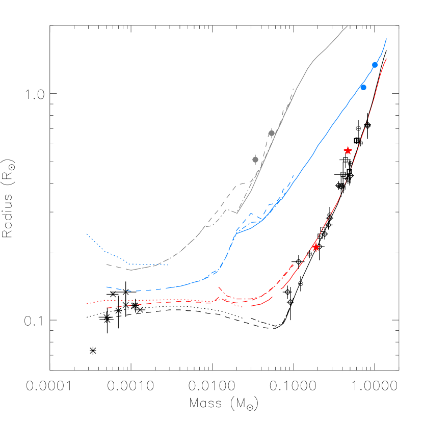
Figure 1: Observational constraints on the mass-radius relation. Black circles represent interferometric measurements of field stars (Lane et al., 2001; Ségransan et al., 2003), and all other symbols represent members of eclipsing binary or transiting systems: the secondaries of field F-M or G-M systems from the OGLE survey (Bouchy et al., 2005; Pont et al., 2005) are shown as black diamonds, field M-M systems (Metcalfe et al., 1996; Torres & Ribas, 2002; Ribas, 2003; Maceroni & Montalbán, 2004; Creevey et al., 2005; López-Morales & Ribas, 2005) as black squares, and planets that transit across field stars (Charbonneau et al. 2000; Henry et al. 2000; Konacki et al. 2003; Bouchy et al. 2004; Konacki et al. 2004; Pont et al. 2004; Alonso et al. 2004; Konacki et al. 2005; Bouchy et al. 2005; Sato et al. 2005; McCullough et al. 2006) as black crosses. The red filled stars represent the NGC 1647 system (Hebb et al., 2006), the blue filled circles the Ori 1c system (Stassun et al., 2004) and the grey filled circles the ONC double brown dwarf system (Stassun et al., 2006). The solid, dashed, dot-dash and dotted lines respectively show the NEXTGEN (Baraffe et al., 1998), DUSTY (Chabrier et al., 2000) and COND (Baraffe et al., 2003) models of the Lyon group and the non-grey models of Burrows et al. (1997) for 1 Gyr (black), 150 Myr (red), 10 Myr (blue) and 1 Myr (grey).

In recent years, the discovery of a number of eclipsing binaries with at least one M-star component (Torres & Ribas, 2002; Ribas, 2003; Maceroni & Montalbán, 2004; Creevey et al., 2005; López-Morales & Ribas, 2005; Bouchy et al., 2005; Pont et al., 2005) together with interferometric radius measurements of a number of field dwarfs in the late-K to mid-M spectral range (Lane et al., 2001; Ségransan et al., 2003), have vastly improved the available constraints on the low-mass main sequence mass-radius relation, down to the very edge of the brown dwarf regime (Pont et al., 2005, 2006). These form a tight sequence which is relatively well reproduced by evolutionary models of low-mass stars such as those of Baraffe et al. (1998), as illustrated in Figure 1.

On the other side of the ‘brown dwarf desert’, the ten planets that are currently known to transit their parent star (Charbonneau et al. 2000; Henry et al. 2000; Konacki et al. 2003; Bouchy et al. 2004; Konacki et al. 2004; Pont et al. 2004; Alonso et al. 2004; Konacki et al. 2005; Bouchy et al. 2005; Sato et al. 2005; McCullough et al. 2006) present very diverse properties even at late ages, some falling above or below the locus predicted by models of isolated gaseous objects without a solid core (Burrows et al., 1997; Baraffe et al., 2003). Evolutionary models incorporating solid cores and the effects of tidal interaction with and irradiation by the parent star are now successfully reproducing the radii of most of them, except for HD 209458b (the most massive of the group of two large planets on Figure 1), which remains a challenge (Laughlin et al., 2005; Baraffe et al., 2005).

However, only six data points so far constrain the mass-radius relation from $1\,M_{\sun}$ downwards at ages younger than 1 Gyr. The first pair is a $1.0+0.7\,M_{\sun}$ eclipsing binary discovered by Stassun et al. (2004), thought to belong to the Ori 1c association and with an estimated age of 5–10 Myr (shown in blue on Figure 1). The next is a double M-star eclipsing binary found by Hebb et al. (2006) in the 150 Myr old open cluster NGC 1647 (shown in red on Figure 1). Finally, the recent discovery by Stassun et al. (2006) of a double brown dwarf eclipsing binary in the $\sim 1$ Myr Orion Nebula Cluster (shown in grey on Figure 1) represents, to the best of our knowledge, the first direct constraint on the mass-radius relation for brown dwarfs at any age. All of these objects fall significantly above the main-sequence relation, highlighting the importance of age in this diagram.

Stassun et al. (2004) and Hebb et al. (2006) compared the properties of the first two EBs to a number of evolutionary models in the literature – some of the most widely used are illustrated on Figure 1 – but none were found that fit both components of each system simultaneously (although the discrepancy is not clearly visible on Figure 1, the relevant isochrone systematically misses the error box on at least one of the components, a problem which is not solved either by adjusting the age or using a different set of isochrones). While the masses and radii of the latter ONC EB are in reasonable agreement with theoretical models for the assumed age of the system, the (less massive, fainter) secondary appears to be hotter than the primary. None of the models predict this surprising result.

Monitor has been designed to attempt to populate the entire section of the diagram in Figure 1 which lies above the main sequence line, across the entire range of masses shown.

1.2 Young low-mass binaries

Aside from improving our understanding of the mass-radius relation, simply measuring dynamical masses for stars and brown dwarfs with known distances and ages provide important constraints on the evolutionary models of these objects. Dynamical masses can be obtained by spectroscopic follow-up of eclipsing binaries or by direct searches for spectroscopic binaries, which is foreseen in those clusters that lend themselves to it as an extension of the main, photometric part of the Monitor project.

The distribution of stellar masses is a direct result of the star formation process. Measurements of individual stellar and sub-stellar masses provide crucial information on the structure and evolution of these objects (Lastennet & Valls-Gabaud, 2002) and measurements of the mass function of a population allow us to understand the detailed physics of the star formation mechanism as a whole.

The stellar mass function has long been studied (e.g. Salpeter, 1955), but only recently are we pushing down into the low-mass and sub-stellar regimes (Hillenbrand & Carpenter, 2000; Barrado y Navascués et al., 2002; Luhman et al., 2003; Moraux et al., 2003; Slesnick et al., 2004). Luminosity functions can be reliably determined, but the more fundamental mass functions remain uncertain, particularly at the low-mass end and for young ages. In this regime, conversion of a luminosity function to a mass function relies heavily on theoretical stellar evolutionary models which infer stellar masses and ages from derived luminosities and temperatures. These models suffer from large uncertainties at low masses, because of the complexity of modeling stellar atmospheres below 3800 K, where molecules dominate the opacity and convection dominates energy transport (Hillenbrand & White, 2004), and at early ages, because of the lack of observational constraints on the initial conditions (Baraffe et al., 2002).

Stellar and sub-stellar masses can only be determined through investigation of an object’s gravitational field, and the small subset of objects in which mass determination is possible are used to calibrate evolutionary models for all stars. A small (but growing) number of low-mass main sequence stars have empirically measured masses (Delfosse et al., 2000; López-Morales & Ribas, 2005), however the models are not fully constrained at young ages or at the lowest masses (brown dwarf regime) due to the scarcity of measurements, which only increases towards the brown dwarf domain (Bouy et al., 2004). There are only a handful of dynamical mass constraints for low-mass PMS objects (Delfosse et al., 2000; Hillenbrand & White, 2004; Stassun et al., 2004; Close et al., 2005; Stassun et al., 2006), and these constitute a growing body of evidence suggesting that current evolutionary models systematically under-predict masses of pre-main sequence stars (for a given temperature or luminosity) below $0.5\,M_{\sun}$.

More dynamical mass measurements of young very-low-mass stars and BDs of known age are clearly needed to anchor the theory. The only way to do this in a systematic way is by searching for binaries in young clusters and star forming regions. As the low-mass members of clusters which are rich enough to provide statistically significant numbers of targets tend to be too faint for the current capabilities of direct imaging and astrometric searches, spectroscopy (radial velocities) and photometry (occultations) appear to be the most promising methods.

1.3 Planets around young stars

The detection of young planets not only helps to anchor evolutionary models of planets – as constrained by the mass-radius relation – but also improves our understanding of the formation of planetary systems and of the dynamical processes that take place early on in their evolution.

The past decade has seen the discovery of nearly 200 extra-solar planets (ESPs), mainly via the radial velocity (RV) method. Statistical studies of these systems (see e.g. Udry et al., 2003; Santos et al., 2003; Eggenberger et al., 2004) provide constraints on formation and migration scenarios, by highlighting trends in the minimum mass-period diagram, or in incidence rate versus parent star metallicity. However, almost all the currently known planets orbit main sequence field stars whose ages can be determined only approximately. Any detection of a planet around a pre-main sequence star would provide much more direct constraints on formation and migration timescales, particularly around a star aged 10 Myr or less, the timescale within which near-infrared observations (Haisch et al., 2001) and accretion diagnostics (Jayawardhana et al., 2006) indicate that proto-planetary discs dissipate.

The only known planetary mass companion within that age range is the companion to 2MASS 1207334–393254, a member of the $\sim 8$ Myr association TW Hydra (Chauvin et al., 2005). This system’s properties are more akin to those of binaries than star-planet systems separation (see e.g. Lodato et al., 2005), and the detection of other, more typical planetary systems in this age range is a major possible motivation for the Monitor project.

1.4 Existing open cluster transit surveys

The potential impact of any transit discovery in an open cluster, together with other advantages such as the fact that an estimate of their masses can usually be determined from their broad-band colours alone, have motivated a number of transit searches over the last few years. These include the UStAPS (the University of St Andrews Planet Search, Street et al. 2003; Bramich et al. 2005; Hood et al. 2005, EXPLORE-OC (von Braun et al., 2005), PISCES (Planets in Stellar Clusters Extensive Search, Mochejska et al. 2005, 2006) and STEPSS (Survey for Transiting Extrasolar Planets in Stellar Systems, Burke et al. 2006). Some of these surveys are still ongoing, but no detection of a transiting planet confirmed by radial velocity measurements has been announced so far. These non-detections are at least partially explained by initially over-optimistic estimates of the detection rate, and by the smaller than expected number of useful target stars per cluster field.

A direct comparison of Monitor to the existing surveys in terms of observational parameters is somewhat complex, because of the range of telescopes and strategies adopted in Monitor (see Section 2). However, broadly speaking, Monitor uses similar observing cadence as previous surveys, but has to use generally larger telescopes (2.2–4 m rather than 1 to–2.5 m), because of its focus on young clusters, which limits the choice of target distances. This implies that Monitor surveys are somewhat deeper, but that it is not possible to obtain continuous allocations of several tens of nights (as the telescopes in question are in heavy demand). The number of cluster members monitored with sufficient photometric precision to detect occultations in each cluster varies from several hundred to over 10 000, i.e. it is in some cases lower than the typical numbers for other surveys, and in others higher.

More importantly, aside from these observational considerations, there are fundamental differences between Monitor and other open cluster transit surveys. The first is that it focuses on younger (pre-main sequence) clusters (the youngest target clusters of the above surveys are several hundred Myr old). Any detections arising from Monitor would thus have a different set of implications to those arising from a survey in older clusters. The second is that Monitor was designed to target lower mass stars, because that is where constraints on evolutionary models and companion incidence were the scarcest and because the youth of our targets made it possible (low mass stars being brighter at early ages, compared to their higher mass counterparts). Finally, while the aforementioned surveys have been designed with the explicit goal of searching for planetary transits, the detection of eclipsing binaries was considered as important as that of planetary transits when choosing Monitor targets and observing strategies. As we shall see, detections of binaries are expected to far outnumber detections of planets. Compared to other open cluster transit surveys, Monitor thus explores a very different area of the complex, multi-dimensional parameter space of double star and star-planet systems.

1.5 Additional science

The proposed observations are also ideally suited to measuring rotational periods for various ages and masses. The age distribution of our target clusters samples all important phases of the angular momentum evolution of low-mass stars, including the T Tau phase where angular-momentum exchange with an accretion disk is important, the contraction onto the zero-age main sequence, and the beginning of the spin-down on the main sequence. The high time cadence and relatively long baselines required by the principal science goal (the search for occultations) implies excellent sensitivity to periods ranging from a fraction of a day to over ten days, and longer in the case of our ‘snapshot mode’ observations (see Section 2.2), while our photometric precision should allow us to measure periods right across the M-star regime, and into the brown dwarf domain in some cases. The rotational analysis of several of our clusters is already complete (M34, Irwin et al. 2006) or nearing completion (NGC 2516, Irwin et al. in prep., NGC 2362, Hodgkin et al. in prep.), and we refer the interested reader to those papers for more details.

In addition, we will also use the light curves collected as part of the Monitor project to search for and study other forms of photometric variability in the cluster members, such as flaring, micro-flaring and accretion related variability. At a later date, the exploitation of the light curves of field stars falling within the field-of-view of our observations is also foreseen, including searching for occultations and pulsations.

The target selection and survey design for Monitor are described in Section 2. In Section 3, we performed a detailed semi-empirical investigation of the number and nature of detections expected in each target cluster. In Section 4, we describe our follow-up strategy and incorporate the limits of feasible radial velocity follow-up into the detection rate estimates of the previous Section. The present status of the observations, analysis and follow-up are briefly sketched out in Section 5.

2 The Monitor photometric survey

2.1 Target selection

Table 1: Basic properties of the Monitor target clusters. may need to change age of ic4665

Name	RA	Dec	Age	$(M-m)_{0}$	$E(B-V)$	$\Omega_{\rm C}$	$I_{\rm BD}$	$M_{20}$	$N^{\prime}$	$\Omega^{\prime}$	$M_{\rm L}^{\prime}$	$M_{\rm H}^{\prime}$	Ref
	$hh~{}mm$	$dd~{}mm$	(Myr)	(mag)	(mag)	(°)	(mag)	($M_{\sun}$)2		(°)	($M_{\sun}$)	($M_{\sun}$)
ONC	05 35	$-$05 23	1	8.36	0.05	$\sim 0.35$	16.78	0.02	$1600$	$0.5~{}$	$0.1~{}~{}$	$50~{}~{}~{}$	a
							16.78	0.02	$500$	$0.07$	$0.02~{}$	$0.5~{}$	b
NGC 2362	07 19	$-$24 57	5	10.85	0.10	$\sim 0.15$	20.31	0.10	$500$	$0.11$	$0.11~{}$	$0.65$	c,d
$h$ & $\chi$ Per	02 20	$+$57 08	13	11.85	0.56	$2\times\sim 0.05$	22.85	0.35	$279$	$1.0~{}$	$4.0~{}~{}$	$15~{}~{}~{}$	e
IC 4665	17 46	$+$05 43	28	7.72	0.18	$\sim 4.0~{}$	19.42	0.55	$150$	$4.0~{}$	$0.02~{}$	$0.2~{}$	g,h
NGC 2547	08 10	$-$49 10	30	8.14	0.06	$\geq 0.85$	19.21	0.05	$700$	$0.85$	$0.035$	$0.9~{}$	f
Blanco 1	00 04	$-$29 56	90	7.07	0.01	$\geq 2.3~{}$	19.15	0.06	$300$	$2.3~{}$	$0.03~{}$	$0.6~{}$	i
M50	07 02	$-$08 23	130	10.00	0.22	$\sim 0.19$	22.68	0.25	$2050$	$0.35$	$0.05~{}$	$0.55$	j
NGC 2516	07 58	$-$60 52	150	8.44	0.10	$\geq 2~{}~{}~{}$	20.0	0.08	$1200$	$2.0~{}$	$0.02~{}$	$0.2~{}$	k,l
M34	02 42	$+$42 47	200	8.98	0.10	$\sim 0.55$	21.7	0.11	$89$	$0.55$	$0.9~{}~{}$	$2.5~{}$	k,m

Notes: The age, distance modulus $(M-m)_{0}$ and reddening $E(B-V)$ of each cluster were taken from the literature ($1^{\rm st}$ entry in the ‘Ref’ column if more than one is present), where they were generally derived from isochrone fitting to the cluster sequence on optical (and in some cases near-IR) colour-magnitude diagrams. The cluster area $\Omega_{\rm C}$ is given approximately, based on the area covered in the reference used and whether the entire extent of the cluster was covered or not. The apparent magnitude $I_{\rm BD}$ at the Hydrogen-burning mass limit of $0.072\,M_{\sun}$ and the mass $M_{20}$ corresponding to $I=20$ were deduced from the cluster ages, distance moduli and reddening values using the models of Baraffe et al. (1998) and the extinction law of Binney & Merrifield (1998). The approximate number $N^{\prime}$ of known or candidate cluster members prior to starting the Monitor project was also taken from the literature ($2^{\rm nd}$ entry in the ‘Ref’ column if more than one is present). Two separate values are given for the ONC as they correspond to widely different mass ranges ($M_{\rm L}^{\prime}$ to $M_{\rm H}^{\prime}$) and spatial coverage ($\Omega^{\prime}$). Where the reference used quoted a number of candidate members (generally selected from optical CMDs using theoretical PMS isochrones), but also gave an estimate of the degree of contamination by field stars, we give here the number of candidate members corrected for contamination. The references are: (a) Hillenbrand (1997); (b) Hillenbrand & Carpenter (2000); (c) Moitinho et al. (2001); (d) Dahm (2005); (e) Slesnick et al. (2002); (f) Jeffries et al. (2004); (g) Manzi (2006) (h) de Wit et al. (2006); (i) Moraux et al. (2006); (j) Kalirai et al. (2003); (k) Sarajedini et al. (2004); (l) Moraux et al. (in prep.) (m) Ianna & Schlemmer (1993). Where 2 references are given on one line, the first was used for the age, distance and reddening and the second for the membership estimate.

The initial selection criteria for our target clusters were that their age be $\leq 200$ Myr, that the apparent $I$-band magnitude at the Hydrogen-burning mass limit be $\leq 21$ (this implies an age-dependent distance limit), and that at least a few hundred PMS cluster members could conveniently be surveyed in a single field of one of the available wide-field optical cameras on 2 to 4 m telescopes (i.e. that the cluster should be compact and rich enough, with a well-studied low-mass pre-main sequence population). These criteria were initially applied to a list of open clusters and star forming regions compiled from the literature, the WEBDA Open Cluster database and several open cluster atlases. This yielded a list of top-priority clusters fulfilling all of the above criteria (Orion Nebula Cluster, NGC 2362, NGC 2547, NGC 2516), which was then completed with clusters which fulfilled only some of the criteria but filled a gap in the age sequence constituted by the original set of targets and/or had a right ascension which was complementary to that of another cluster, allowing them to be observed simultaneously by alternating between the two ($h$ & $\chi$ Per, IC 4665, Blanco 1, M50, M34).

Some obvious candidates were excluded because of their large angular extent (e.g. $\alpha$ Per and the Pleiades) or because they were not rich enough (e.g. IC 348). NGC 2264 will be the target of a continuous 3-week ultra-high precision monitoring program in the framework of the additional program of the CoRoT space mission, which will far outstrip the time sampling and photometric precision achievable from the ground, and was therefore left out of the present survey. Two clusters, NGC 6231 and Trumpler 24, appeared to be promising targets but had poorly studied low mass populations, and a preliminary single-epoch multi-band survey was undertaken to investigate their low-mass memberships. Depending on the results of this survey, these two clusters may be added to the list of Monitor targets.

The most up to date estimates of the properties (age, distance, reddening, membership) of the current set of target clusters that were found in the literature are summarised in Table 1. Figure 2 summarises the age and distance distributions of the target clusters together with the number of objects monitored in each and the degree of completion of the monitoring to date.

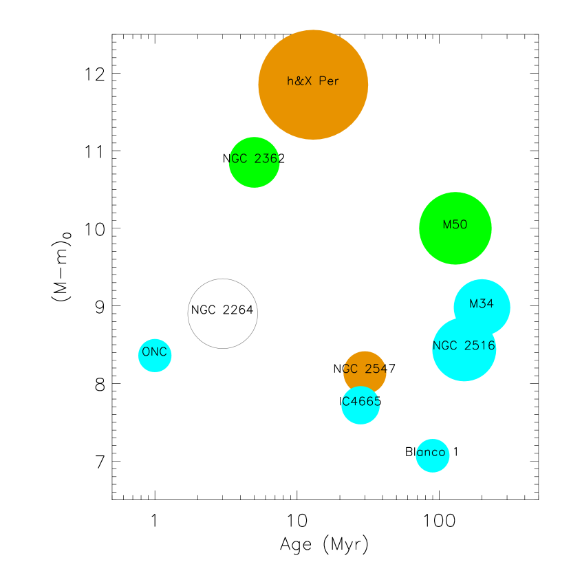
Figure 2: Age and distance distribution of the Monitor target clusters. The size of the circle representing each cluster scales with $N^{0.3}$, where $N$ is the number of non-saturated cluster members monitored with better than 5% precision (see Section 3.2), and the colour-coding indicates whether we have obtained all (green), some (blue) or none (orange) of we have obtained all (green), some (blue) or none (orange) of the data for that cluster at the time of writing. For comparison, we also show NGC,2264 (hollow circle), which will be the target of a CoRoT monitoring campaign.

2.2 Observing strategy

Table 2: Observations of the Monitor targets to date.

Name	Tel	FOV	$N_{\rm P}$	$t_{\rm exp}$	$\delta t$	$I_{\rm sat}$	$I_{5\%}$	$t_{\rm req}$	$t_{\rm all}$	$t_{\rm tot}$	$T$	filter	semester/
		(°)		(sec.)	(min)	(mag)	(mag)			(h)	(days)		period
ONC	INT	$0.29$	1	30	$3.5$	13.0	19.0	40 n	40 n	55.5	70	$V,i$	04B–06B
NGC 2362	CTIO	$0.38$	1	75	$6.6$	15.5	20.5	14 n	14 n	93.6	360	$i$	05A–06A
$h$ & $\chi$ Per	CFHT	$1.0~{}$	1	120	$10~{}~{}$	15.5	20.5	100 h	40 h	0.0	—	$I$	05B,06B
	KPNO	$0.35$	2	75	$9~{}~{}$	15.5	20.5	8 n	8 n	0.0	—	$i$	06B
IC 4665	CFHT	$1.0~{}$	4	120	$14~{}~{}$	15.5	20.5	100 h	40 h	16.1	136	$I$	05A
NGC 2547	2p2	$0.29$	2	120	$15~{}~{}$	13.0	19.5	100 h	100 h	0.0	—	$I$	P75–P77
Blanco 1	2p2	$0.29$	3	120	$15~{}~{}$	13.0	19.5	100 h	100 h	6.6	26	$I$	P75–P78
M50	CTIO	$0.38$	1	75	$6.6$	15.5	20.5	14 n	14 n	93.6	360	$i$	05A–06A
NGC 2516	CTIO	$0.38$	3	75	$8.8$	15.5	20.5	8 n	8 n	68.6	400	$i$	06A
M34	INT	$0.29$	1	30	$3.5$	13.0	19.0	10 n	10 n	18.0	10	$V,i$	04B
	CFHT	$1.0~{}$	1	120	$10~{}~{}$	15.5	20.5	100 h	40 h	0.0	—	$I$	05B,06B
	KPNO	$0.35$	1	75	$9~{}~{}$	15.5	20.5	8 n	8 n	0.0	—	$I$	06B

Notes: The different telescope/instrumentation combinations used are: INT: Isaac Newton Telescope (2.5 m) with the Wide Field Camera; CTIO: Blanco telescope (4 m) at Cerro Tololo Interamerican Observatory with MosaicII; CFHT: Canada-France-Hawaii Telescope (3.6 m) with MegaCAM; KPNO: Mayall telescope (4 m) at Kitt Peak National Observatory with Mosaic; 2p2: ESO/MPI telescope (2.2 m) at La Silla Observatory with the Wide Field Imager. $N_{\rm P}$ refers to the number of pointings used for each cluster, $t_{\rm exp}$ to exposure time used for each pointing, and $\delta t$ to the resulting interval between consecutive observations. $I_{\rm sat}$ and $I_{5\%}$ are the approximate $I$-band magnitudes at which saturation occurs and the frame-to-frame rms of the light curves is $\sim 5$%, respectively. The total observing time requested ($t_{\rm req}$) and allocated ($t_{\rm al}$) to date for each cluster are given in nights for visitor mode observations and hours for snapshot or service mode observations. The total time on target $t_{\rm tot}$, which is equal to the duration of the light curves produced so far with the daily gaps removed, is given in hours in all cases (and should be compared with the target of $\sim 100$ h). $T$ refers to the total time span of the light curves to date. The completion rate of our INT runs to date has been very partial due to adverse weather conditions. $h$ & $\chi$ Per and M34 are targeted with two and three different telescopes respectively, covering different magnitude ranges. The semester/period column refers to the telescope time allocation semester or period (P75 corresponds approximately to 05B).

The optimal observing strategy for a survey like Monitor is a complex combination of a large number of considerations including photometric precision, number of objects monitored in a given mass range, and time sampling. The different ages, physical sizes and distances of our target clusters, as well as their positions on the sky, also come into play, as do considerations of a more practical nature, such as the need to find clusters of compatible right ascension to observe in one given run or cycle. In general, the size of telescope to use for a given cluster was determined by the magnitude of the Hydrogen burning mass limit inferred from the cluster age and distance, given that we wished to monitor objects near this limit with precision sufficient to detect occultations, i.e a precision of a few percent at worst. The nearest and brightest clusters such as the ONC are suitable targets for 2 m class telescopes, whereas the more distant or older clusters are more suitable for 4 m class telescopes. While some attempt was made at matching detector field-of-view (FOV) to cluster angular size, this was not always possible – there is currently no equivalent of the 1 sq.deg. FOV of CFHT/MegaCAM in the South, so that our large Southern targets were monitored using a dither pattern of 3 or 4 pointings.

Exposure times were adjusted to ensure a precision of 1% or better down to the cluster Hydrogen burning mass limit (HBML) or the apparent magnitude $I=19$, whichever was the brightest, with the caveat that exposures were kept sufficiently long to avoid being excessively overhead-dominated. The $I\leq 19$ limit arises from the need to perform radial velocity follow-up of all candidates to determine companion masses, which becomes impractical even with 8 m class telescopes beyond that limit.

Adequate sampling of the event is vital to ensure the detection is of an occultation and not of some other type of temporary dip in flux. In conventional planetary transit searches around field stars, the shape of the candidate transit event is used to minimise contamination by stellar eclipses. In the case of Monitor, eclipses as well as transits are of interest, but it is important to maximise the amount of information that can be extracted from the light curve. All Monitor campaigns were designed to ensure that the interval between consecutive data points be less than 15 min, and preferably closer to 5 min. The first value ensures that the duration of the shortest occultations of interest ($\approx 1$ h) is resolved, while the second ensures that the ingress and egress is resolved. The sampling rates are similar to those of other ground- and space-based transit surveys, e.g. COROT.

Some of the telescopes of interest offer a queue scheduled service program. This is not generally used for transit surveys because there is no way to control the distribution of the observations in time and because it is only possible to guarantee continuous observing over a short duration – generally 1 h. The accepted wisdom has been that one must observe continuously for at least the duration of an occultation to ensure that events are observed completely enough. On the other hand, service mode observations present a significant advantage: they allow us to make use of the relatively lax observing conditions requirements of our program. As relative rather than absolute photometric accuracy is the key, and our fields are not excessively crowded, the program can be carried out in moderate seeing (up to 1.5″) and partial transparency. This makes it more feasible to request large amounts of time on the appropriate telescopes, which are generally heavily oversubscribed. It should also improve the sensitivity to long periods, as the data will be spread over an entire season, which is particularly relevant for secondary science goals such as the search for photometric rotation periods. Where such a mode was available, we therefore requested queue-scheduled observations.

There is a risk associated with such a decision, because any occultation detected in this mode is likely to be incomplete, and the number of distinct observations taken during a single occultation will be small – typically 4 at most. Additionally, observed occultations may be separated by long periods without data, and our ability to detect them by phase-folding the light curves will depend on the long-term stability of the instrument and on the presence of any additional long-timescale variability (e.g. starspots), which are difficult to estimate a priori. Some of our target clusters will be observed in both queue scheduled and visitor modes, and we will use these datasets to perform an a posteriori evaluation of the relative advantages of each mode for occultation surveys.

The total time allocation requested for each cluster was chosen to ensure that the probability to observe at least three separate occultation events for periods up to 5 days should exceed 50%. We carried out Monte Carlo simulations of occultation observability under various assumptions regarding the distribution of the observations in time, including not only visitor mode observations with an adjustable number of runs of variable duration, but also service mode observations organised in fixed duration ‘blocks’ distributed semi-randomly. Interestingly, we found that, provided the time span of the observations was significantly longer than the orbital periods under consideration (we investigated periods up to 10 d), the relevant quantity was the total time $t_{\rm tot}$ spent on target, and that a total of $\sim 100$ h for each target was appropriate. We therefore requested 100 h per cluster in service mode. When only visitor mode was available, we requested a number of nights totaling up to slightly more than 100 h to account for time lost to weather, with the allocation being splits into two or more runs to ensure that the time span of the light curves was significantly longer than 5 days.

The observations of each cluster are summarised in Table 2. The telescope/instrument combinations used are: the 2.2m MPI/ESO telescope (2p2) with the Wide Field Imager (WFI), the 2.4 m Isaac Newton Telescope (INT) with the Wide-Field Camera (WFC), the 3.6 m Canada-France-Hawaii Telescope (CFHT) with the MegaPrime/MegaCam camera, the 4 m Blanco telescope at Cerro Tololo Interamerican Observatory (CTIO) with the Mosaic II imager, and its northern twin the 4 m Mayall telescope at Kitt Peak National Observatory (KPNO) with the Mosaic imager. The approximate magnitude limits $I_{\rm sat}$ and $I_{\rm 5\%}$ and interval between consecutive observations $\delta t$ were evaluated from the data themselves wherever possible, and by analogy with other clusters observed with the same set-up and strategy in the cases where data are not yet available. The table clearly shows that, although the total amount of time allocated to the survey in the vast majority of the clusters matches or exceeds the requirement of 100 h, the actual amount of data collected often falls short of this requirement. This is due to adverse weather conditions in the case of visitor mode observations, and to lower completion rates than expected for the queue-scheduled programs, due to the low priority assigned to snapshot programs at the CFHT and technical problems delaying Monitor observations on the ESO 2.2 m. The sensitivity estimates presented in Section 3.5.4 are re-computed after each observing run (or delivery of data from service mode programs) and used to evaluate whether an application for more data is needed.

2.3 Data reduction and light curve production

For a full description of our data reduction steps, the reader is referred to Irwin et al. (in prep.). Briefly, we use the pipeline for the INT wide-field survey (Irwin & Lewis, 2001) for 2-D instrumental signature removal (crosstalk correction, bias correction, flat-fielding, defringing) and astrometric and photometric calibration. We then generate the master catalog for each filter by stacking a few tens of the frames taken in the best conditions (seeing, sky brightness and transparency) and running the source detection software on the stacked image. The resulting source positions are used to perform aperture photometry on all of the time-series images. We fit a 2-D quadratic polynomial to the residuals in each frame (measured for each object as the difference between its magnitude on the frame in question and the median calculated across all frames) as a function of position, for each of the detector CCDs separately. Subsequent removal of this function accounts for effects such as varying differential atmospheric extinction across each frame. We typically achieve a per data point photometric precision of $\sim 2-5\ {\rm mmag}$ for the brightest objects, with RMS scatter $<1\%$ over a dynamic range of approximately 4 magnitudes in each cluster.

Photometric calibration of our data is carried out using regular observations of Landolt (1992) equatorial standard star fields in the usual way. This is not strictly necessary for the purely differential part of a campaign such as ours, but the cost of the extra telescope time for the standards observations is negligible, for the benefits of providing well-calibrated photometry (e.g. for the production of CMDs). In most of our target clusters we use CMDs for membership selection, produced by stacking all observations in each of $V$ and $i$ that were taken in good seeing and sky conditions (where possible, in photometric conditions). The instrumental $V$ and $i$ or $I$ measurements are converted to the Johnson-Cousins system of Landolt (1992) using colour equations derived from a large number of standard star observations.

2.4 Search for occultations

Although we intend to search for occultations in all of our light curves in the long term, in the first instance we focus on likely cluster members. In most cases, previous membership surveys – based on proper motion, spectroscopy or photometry – are not as deep as our CMDs, and therefore we carry out our own membership selection.

In general, neither theoretical evolutionary models such as those of Baraffe et al. (1998) nor empirical sequences such as Reid & Gilmore (1982) and Leggett (1992) produce a good fit to the visible cluster sequence on the $V$, $V-I$ CMD. Candidate cluster members are therefore selected by defining an empirical main sequence, and moving this line perpendicular to the mean gradient of the main sequence, toward the faint, blue end of the diagram, by a constant adjusted by eye plus a small multiple of the photometric error in $V-I$. The interested reader is referred to Irwin et al. (2006) for more details and an example of this procedure applied to our INT observations of M34.

Before searching for occultations, one must circumvent a major obstacle: the intrinsic variability that affects the light curves of almost all stars in the age range of the Monitor clusters at the level of a few mmag to a few percent. When the major source of this variability is the rotational modulation of starspots, it leads to smooth variations that can be adequately modeled and subtracted before the occultation search proceeds. We routinely search for this modulation, using a sine-fitting procedure (see e.g. Irwin et al., 2006), prior to starting the occultation search. When the sine-fitting process leads to a detection, a starspot-model is fitted to the light curve(s) at the detected period, following the approach of Dorren (1987). Even in the absence of a direct detection of rotational modulation, any variability on time-scales significantly longer that the expected duration of occultations (i.e. variability on timescales of a day and longer) is filtered out using Fourier-domain filters (Carpano et al., 2003; Aigrain & Irwin, 2004; Moutou et al., 2005).

After pre-filtering, we search the filtered light curves for occultations automatically using an algorithm based on least-squares fitting of two trapezoid occultations of different depths but identical internal and external durations, where the internal and external durations are the time intervals between the $2^{\rm nd}$ and $3^{\rm rd}$ contact, and the $1^{\rm st}$ and $4^{\rm th}$ contact, respectively (Aigrain et al. in prep.). Note that a single box-shaped transit is a special case of the double trapezoid where one of the occultations has zero depth and the internal and external durations are the same. The double trapezoid algorithm directly provides an estimate of the basic parameters of the occultation which can be used, together with an estimate of the primary mass based on its optical and near-IR (2MASS) magnitudes if available, for a preliminary estimate of the radius ratio of any detected systems.

In our youngest clusters, a variable fraction of the light curves are affected by rapid, semi-regular variability which is not clearly periodic (and hence not effectively detected by the sine-fitting procedure or removed by the starspot fit) and overlaps with any occultation signal in frequency space (and hence is not removed by the Fourier domain filters unless at the expense of the signals of interest themselves). We have found – from our preliminary investigation of the ONC data collected to date – that visual inspection of the light curves is the most effective way of finding occultations in such cases. Those variations are thought to arise from accretion- and time-varying activity-related effects, and concern primarily classical T Tau stars. The fraction of stars with inner discs (estimated from near-IR excesses, Haisch et al. 2001) therefore provides a rough estimate of the fraction of light curves of members we should expect to display such variability: $\sim 60$% for the ONC, $\sim 10$% for NGC 2362, and very small for all other clusters.

The calculations described in the present paper assume the double trapezoid fitting algorithm is used in all cases, and essentially ignore the effects of any variability that is not removed by the pre-filtering stage. One should keep in mind that most of the occultations we expect will be deep, and therefore their detectability will be unaffected even by variability at the level of a few percent. The events for which we do expect residual variability to play a role are transits of planets around the youngest and highest mass stars – and we shall see in Section 4.2 that these are also those for which the limitations imposed by the need to carry out radial velocity follow-up are most stringent. We do plan to estimate in detail the impact of residual intrinsic variability on our ability to detect occultations by injecting artificial events into the real pre-filtered light curves for each cluster, and repeating the detection process, but this is beyond the scope of the present paper.

3 Expected number of detections

A number of recent articles have explored the detection biases of field transit surveys and the impact of the observing strategy on their yield. Pont et al. (2005) analysed a posteriori the planetary transit candidates produced by the OGLE II Carina survey (Udalski et al., 2002, 2003) in the light of the results of the radial velocity follow-up, and highlighted the impact of correlated noise on timescales similar to the duration of a typical transit. Pont et al. (2006, submitted) then developed a formalism to model the correlated noise and account for its influence on expected yields of transit surveys. In parallel, Gaudi (2005); Gaudi et al. (2005) developed an analytical model of the number of detections expected for a given survey. Both groups found the results of transit surveys to date to be in agreement with those of radial velocity surveys, once the biases were properly accounted for. Pepper & Gaudi (2005a) adapted the formalism of Gaudi (2000) to the special case of cluster transit searches, and concluded that such searches may allow the discovery of ‘Hot Neptunes’ or ‘Hot Earths’ from the ground (Pepper & Gaudi, 2005b).

One might therefore envisage applying the prescription of Pepper & Gaudi (2005a) to the Monitor project to evaluate the sensitivity of the survey as a whole and in individual clusters. However, it relies on certain assumptions which hold for planetary transits, but break down for larger and more massive secondaries, as do all the analytical methods proposed so far. For example, when dealing with stellar or brown dwarf companions, the secondary mass is no longer negligible compared to the primary mass. Also, grazing occultations – usually ignored in the planetary transit case as both rare and hard to detect – become common and detectable, and may in fact represent the majority of detections. Another shortfall of published analytical models is that they make simple assumptions regarding the noise properties of the data, often assuming that the sole contributions to the noise budget are source and sky photon noise, and that the noise is purely white (uncorrelated). Similarly, the time array is generally assumed to consist of regularly sampled ‘nights’, making no allowance for intermittent down time or time lost to weather.

An alternative approach is to carry out Monte Carlo simulations once the data have been fully reduced and analysed, injecting fake occultation events into the light curves and applying the same detection procedure as in the actual occultation search to derive completeness estimates, and hence place constraints on the incidence of companions in a given regime of parameter space. Using such an approach, Mochejska et al. (2005); Weldrake et al. (2005); Bramich & Horne (2006); Burke et al. (2006) derived the upper limits on planet incidence in the field of a star cluster, although the limits were not always stringent enough to constrain formation scenarios because of insufficient target numbers and time sampling. Such a procedure is envisaged in the long run for Monitor targets, but it becomes very time consuming because of the huge variety of occultation shapes and sizes which must be considered.

The purpose of the present work is to gain a global rather than detailed insight into the potential of the Monitor project and the type of systems which we may expect to detect. We have therefore opted for an intermediate approach, based on a semi-analytical model, which aims to incorporate important factors in the detection process, such as the real time sampling and noise budget of the observations (including correlated, or red, noise), while keeping complexity to a minimum by carrying out calculations analytically wherever possible and stopping short of actually injecting occultations into the observed light curves. The calculations were implemented as a set of IDL (Interactive Data Language) programs. Note that we have deliberately excluded two significant factors, namely contamination by non-cluster members and out-of-occultation variability, while the feasibility of radial velocity follow-up is dealt with separately in Section 4.2.

3.1 Procedure

The number of detections expected in a given cluster is evaluated according to:

$$N_{\rm det}=\int\int\int N_{\rm sys}(M)P_{\rm c}P_{\rm o}P_{\rm d}{\mathrm{d}}\log M{\mathrm{d}}x{\mathrm{d}}p$$ (1)

where

• $M$ is the total system mass ($=M_{1}+M_{2}$ where $M_{1}$ and $M_{2}$ are the primary and secondary mass respectively);

• $x$ is the parameter defining the companion. For binaries, we use the mass ratio $q=M_{2}/M_{1}$ as our defining parameter $x$, whereas for planet we use the companion radius $R_{2}$, for reasons explained below;

• $p$ is the orbital period;

• $N_{\rm sys}$ is the number of observed systems with total mass $M$;

• $P_{\rm c}$ is the companion probability. Given that we parametrise our systems according to total mass rather than primary mass (for reasons which are explained below), this is the probability that a system of total mass $M$ is made up of at least 2 components;

• $P_{\rm o}$ is the occultation probability, i.e. the probability that eclipses or transits occur for a given binary or star-planet system;

• $P_{\rm d}$ is the detection probability, i.e. the probability that occultations are detectable if they occur.

We use $M$ and $q$ to parametrise binaries, rather than $M_{1}$ and $M_{2}$, for a number of reasons. Working in terms of $M_{\rm tot}$ is a more natural choice than $M_{1}$ because our surveys do not resolve close binaries, and therefore each source detected on our images must be considered as a potential multiple, rather than as a single star. Additionally, most published mass functions for young clusters (used for estimating $N_{\rm sys}$) are derived from CCD surveys which do not resolve close binaries, and thus correspond to systems rather than single stars. Using $q$ rather than $M_{2}$ is convenient because the companion probability is often parametrised in terms of mass ratio. Similarly, we use radius rather than mass to parametrise the planets. In most cases, the mass of planetary companions is generally negligible compared to that of their parent stars, and the occultation and detection probabilities are thus essentially a function of planet radius. Note that this is no longer the case for the lowest mass primaries, so that we do not neglect the planet mass in general. Instead, we assume a mass of $1\,M_{\rm Jup}$ for all planets in the simulations, whatever their radius, because the mass-radius relation for young planets is both degenerate and ill constrained, as discussed in Section 1.1.

All quantities are computed over a three-dimensional grid of system parameters. The total mass runs from $0.014\,M_{\sun}$ (i.e. just above the planetary mass object limit) to $1.4\,M_{\sun}$ (the approximate mass at which saturation occurs in the oldest, most distant targets), in steps of ${\mathrm{d}}\log M=0.1\,M_{\sun}$. The mass ratio runs from 0 to 1 in steps of ${\mathrm{d}}q=0.05$. The planet radius runs from $0.3\,R_{\rm Jup}$ to $2\,R_{\rm Jup}$ (most evolutionary models of giant extra-solar planets assume initial radii in the range 2–$3\,R_{\rm Jup}$) in steps of ${\mathrm{d}}\log R_{2}=0.1\,R_{\rm Jup}$. The orbital period runs from 0.1 to 100 days for binaries, and 1 to 10 days for planets (no planets are currently known with periods less than 1 day, while the occultation probability becomes negligible for most planets with periods in excess of 10 days).

3.2 Number of systems $N_{\rm sys}$

Table 3: Mass range and number of cluster members monitored in each target cluster.

(a): Cases where $N$ was derived directly from the data.

Name	$\Omega$	$M_{\rm L}$	$M_{\rm H}$	$N$
	(°)	($M_{\sun}$)	($M_{\sun}$)
NGC 2362	$0.38$	$0.07$	$1.14$	587
$h$ & $\chi$ Per (KPNO)	$0.60$	$0.33$	$1.49$	7756
NGC 2547	$0.56$	$0.06$	$0.88$	334
M50	$0.38$	$0.18$	$0.88$	1942
NGC 2516	$1.13$	$0.08$	$0.56$	1214
M34 (INT)	$0.29$	$0.16$	$0.99$	414

(b): Cases where $N$ was derived from the literature or from Monitor data taken with other telescopes.

Name	$N^{\prime}$	$\Omega^{\prime}$	$M_{\rm L^{\prime}}$	$M_{\rm H^{\prime}}$	Ref	$\Omega$	$f_{\Omega}/f^{\prime}_{\Omega}$	$M_{\rm 5\%}$	$M_{\rm sat}$	$N$
		(°)	($M_{\sun}$)	($M_{\sun}$)		(°)		($M_{\sun}$)	($M_{\sun}$)
ONC	500	$0.07$	$0.02$	$0.5~{}$	b	$0.28$	$4.0$	$0.04$	$0.75$	2143
$h$ & $\chi$ Per (CFHT)	7756	$0.60$	$0.33$	$1.49$	(KPNO)	$1.0$	$1.0$	$0.33$	$1.49$	7756
IC 4665	150	$4.0~{}$	$0.03$	$0.2~{}$	h	$4.0~{}$	$1.0$	$0.04$	$0.45$	216
Blanco 1	300	$2.3~{}$	$0.03$	$0.6~{}$	i	$1.17$	$0.5$	$0.06$	$0.8~{}$	148
M34 (CFHT)	414	$0.29$	$0.16$	$0.99$	(INT)	$1.0~{}$	$1.9$	$0.11$	$0.7~{}$	845
M34 (KPNO)	414	$0.29$	$0.16$	$0.99$	(INT)	$0.35$	$1.3$	$0.11$	$0.7~{}$	560

Notes: In the case of the ONC, we have taken the membership estimate from Hillenbrand & Carpenter (2000), rather than Hillenbrand (1997) (which yields a smaller value), because the former corresponds to a mass range more similar to that of the Monitor targets, even though it covers only the central region of the cluster. If the discrepancy is arises from mass segregation (which would lead to a deviation from the log-normal MF adopted to compute $N$ Hillenbrand & Carpenter 2000), then the estimate we used should be close to the true number. It is also within 5% of the number of detected sources in our field, which is reassuring given that few background or foreground field sources are expected in this case.

Within the field of the observations, the expected number of observed system of mass $M$ is

$$N_{\rm sys}(M)\,{\mathrm{d}}\log M=N_{\rm C}\,f_{\Omega}\,\frac{{\mathrm{d}}n}{{\mathrm{d}}\log M}\,{\mathrm{d}}\log M,$$ (2)

where $N_{\rm C}$ is the total number of systems in the cluster, $f_{\Omega}$ accounts for the fact that the field-of-view of the observations may not cover the entire cluster, and $\displaystyle\frac{{\mathrm{d}}n}{{\mathrm{d}}\log M}$ is the normalised system mass function.

Assuming a $1/r$ profile for the density of cluster members,

$$f_{\Omega}=\left\{\begin{array}[]{lcl}1&\textrm{if}&\Omega\geq\Omega_{\rm C}\\ \Omega/\Omega_{\rm C}&\textrm{if}&\Omega<\Omega_{\rm C}\end{array}\right.,$$ (3)

where $\Omega$ and $\Omega_{\rm C}$ are the solid angle covered by the present survey and the total solid angle covered by the cluster, respectively. This assumes that the survey area and the cluster overlap to the greatest possible extent, and the value of $\Omega$ used in practice may differ from that implied by the actual surveyed area to account for departures from this assumption imposed by detector shape or other considerations (such as the need to avoid very bright stars in the centre of some of the clusters, which would otherwise be saturated and contaminate large areas of the detector).

In practice, $N_{\rm C}$ is rarely known directly. However, on can generally find in the literature or, where data is already available, determine from the Monitor data itself, an estimate of the number $N^{\prime}$ of members in a given solid angle $\Omega^{\prime}$ and mass range $M_{\rm L^{\prime}}$ to $M_{\rm H^{\prime}}$, obtained from an earlier membership survey. Assuming that the vast majority of the systems are unresolved – an assumption which holds for all photographic and most CCD surveys, with typical pixel sizes $>0.1\arcsec$ – we then have:

$$N^{\prime}=N_{\rm C}\,f_{\Omega^{\prime}}\int_{M_{\rm L^{\prime}}}^{M_{\rm H^{\prime}}}\frac{{\mathrm{d}}n}{{\mathrm{d}}\log M}\,{\mathrm{d}}\log M,$$ (4)

where $f_{\Omega^{\prime}}$ is the analog, for the earlier survey, of $f_{\Omega}$ for the present one. Therefore, we can write

$$N_{\rm sys}(M)\,{\mathrm{d}}\log M=A\,N^{\prime}\frac{{\mathrm{d}}n}{{\mathrm{d}}\log M}\,{\mathrm{d}}\log M$$ (5)

where $A$ is a normalisation accounting for the difference in spatial coverage and mass range between the previous survey and the present one:

$$A=\frac{f_{\Omega}}{f_{\Omega^{\prime}}}\,\left[\int_{M_{\rm L^{\prime}}}^{M_{\rm H^{\prime}}}({\mathrm{d}}n/{\mathrm{d}}\log M)\,{\mathrm{d}}\log M\right]^{-1}$$ (6)

In some cases, $N^{\prime}$ is available from spectroscopic surveys, but generally we use contamination-corrected numbers of candidate members identified on the basis of their position in colour-magnitude diagrams. Mass segregation is not taken into account.

Several recent determinations of the mass function (MF) of young open clusters (Moraux et al., 2003; Jeffries et al., 2004; de Wit et al., 2006) have concluded that a log-normal distribution is a good fit over the entire mass range of interest to us, from $\sim 1\,M_{\sun}$ to the brown dwarf regime:

$$\frac{{\mathrm{d}}n}{{\mathrm{d}}\log M}\propto\exp\left\{\frac{-\left[\log\left(M/M_{0}\right)\right]^{2}}{2\,\sigma_{M}^{2}}\right\}$$ (7)

where $M_{0}$ is the mean mass and $\sigma_{M}$ the standard deviation, and the constant of proportionality is chosen to ensure the distribution is normalised to 1. Typical values for $M_{0}$ and $\sigma_{M}$ are $0.25\,M_{\sun}$ and $0.52\,M_{\sun}$ respectively (Moraux et al., 2003). A log-normal with similar parameter also provides a good fit to the mass functions derived from Monitor data in the cases of the clusters analysed to date (see e.g. Irwin et al. 2006 for M34 and Irwin et al. in prep. for NGC 2516). As these mass functions result from photometric CCD surveys with moderate spatial resolution, within the orbital distance to which an occultation survey like Monitor is sensitive, multiple systems are blended. This mass function therefore corresponds to the number of systems, which is the quantity of interest to us. There is no need to apply a correction for binarity, which would be required only if our aim was to calculate the distributions of masses for single stars and the individual components of multiple systems, as discussed by Chabrier (2003).

Table 3 lists the overall number $N$ of likely cluster members monitored with useful photometric precision in each cluster, that is between the mass limits $M_{\rm 5\%}$ and $M_{\rm sat}$ corresponding to the magnitude limits of Table 2. Wherever possible, $N$ was derived from the Monitor data itself, following a photometric membership selection procedure described in detail for the case of M34 in Irwin et al. (2006), and including an approximate field contamination correction based on the Galactic models of the Besançon group (Robin et al., 2003). Note that in the case of clusters lying close to the Galactic plane, and hence in crowded fields, we applied a red as well as a blue membership cut, though the former was designed to include the cluster binary sequence. $N$ was obtained by summing the total number of candidate members after contamination correction over the mass range $M_{\rm 5\%}$ to $M_{\rm sat}$. It is worth noting the very rich nature of the twin clusters $h$ & $\chi$  Per. In a study of the high-mass ($M\geq 4\,M_{\sun}$ population, Slesnick et al. (2002) already pointed out that these appear to be roughly 6 to 8 times as rich as the ONC, a finding which is consistent with our own estimate.

Where data is not yet available or not yet analysed, $N$ was computed from the literature or from Monitor surveys of the same cluster with other telescopes according to:

$$N=A\int_{M_{\rm 5\%}}^{M_{\rm sat}}\frac{{\mathrm{d}}n}{{\mathrm{d}}\log M}\,{\mathrm{d}}\log M.$$ (8)

We note that there are sometimes large discrepancies – a factor 2 or more – between the values of $N$ we derive from our own data and those extrapolated from earlier surveys in the literature. These will be discussed in more detail in papers dealing with each cluster in turn, but may arise both from the differences in mass range and spatial coverage between previous surveys and Monitor, and from the uncertainty on the level of contamination of the candidate members lists by field stars. The discrepancies occur in both directions, i.e. membership estimates based on our own data are sometimes below and sometimes above the estimate extrapolated from the literature, and no clear systematic trend emerged from the comparison of the two sets of estimates. The differences highlight the need for spectroscopic confirmation of our photometric membership selection wherever feasible, and for the time being one should treat the values given in Table 3 with caution.

3.3 Companion probability $P_{\rm c}$

3.3.1 Binaries

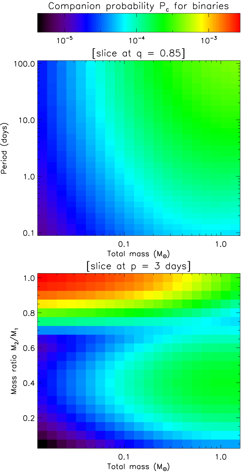
Figure 3: Example two-dimensional cuts through the three-dimensional companion probability for binaries. Top: probability for mass ratio $q=0.85$ as a function of total mass and period. Bottom: probability for period $p=3$ days as a function of total mass and mass ratio. The same logarithmic colour scale is used in both panels.

For stellar and sub-stellar companions, we use the following expression:

$$P_{\rm c}(M,q,p)\,{\mathrm{d}}q\,{\mathrm{d}}p=f_{\rm c}\,\frac{{\mathrm{d}}^{2}p_{\rm c}}{{\mathrm{d}}q\,{\mathrm{d}}p}\,{\mathrm{d}}q\,{\mathrm{d}}p$$ (9)

where $f_{\rm c}$ is the fraction of primaries of mass $M_{1}$ which host one or more stellar or sub-stellar companions, and $p_{\rm c}$ is the probability that a companion to such a primary has mass ratio between $q$ and $q+{\mathrm{d}}q$ and period between $p$ and $p+{\mathrm{d}}p$. $p_{\rm c}$ is normalised to 1 over the range of $q$ and $p$ over which $f_{\rm c}$ is measured.

In a sample of 164 primaries of spectral type F, G or K, Duquennoy & Mayor (1991) found 62 binaries, 7 triples and 2 quadruples, corresponding to a total companion fraction (over the entire period range, as both spectroscopic and visual binaries were considered) of 43%. These authors also found that the distribution of orbital periods is well fit by a log-normal function $\log(p_{0})=4.8$ years and $\sigma_{p}=2.3$ d, noting an excess of short-period binaries ($1\leq P\leq 10$ d) in a statistically young sample of Hyades members. Combining field and open cluster samples of the same range of spectral types, Halbwachs et al. (2003) determined a companion fraction of 14% for orbital periods less than 10 years. This corresponds to a total companion fraction of 47% assuming the Halbwachs et al. (2003) sample follow the period distribution of Duquennoy & Mayor 1991. Halbwachs et al. (2003) also found that the mass ratio distribution was generally bimodal, with a broad, shallow peak stretching over $0.1\la q<0.75$, and a sharper peak centred on $q\sim 1$, whose amplitude was about double that of the other peak, and which was present for short-period binaries ($P<50$ d) only.

For primaries with masses below $0.5\,M_{\sun}$, the situation is less clear. Imaging and radial velocity surveys of early M field dwarfs (i.e. masses around $0.3$–$0.5\,M_{\sun}$) suggest that between 25% and 42% have companions (Henry & McCarthy, 1990; Fischer & Marcy, 1992; Leinert et al., 1997; Reid & Gizis, 1997). For very low-mass stars, the samples are smaller still. Bouy et al. (2003); Close et al. (2003) and Siegler et al. (2005) use high resolution imaging and find companions to around 10-–20% for objects with primary masses around $0.1\,M_{\rm sun}$; again for field dwarfs. However, spectroscopic samples suggest that these studies may be missing significant numbers of close in companions. Maxted & Jeffries (2005) examine a small sample of radial velocity measurements, and estimate that accounting for systems with $a<3$ AU could increase the overall VLM star/BD binary frequency up to 32–45%. Basri & Reiners (2006) survey 53 VLM stars with Echelle spectroscopy, and conclude that the overall binary fraction could be as high as 36%. Pinfield et al. (2005) argue that there is growing evidence that very low mass binaries tend to have shorter periods than their higher mass counterparts, and their mass ratio distribution is more strongly peaked towards $q>0.75$.

Given the level of uncertainty on the multiplicity of low mass stars, we have adopted an overall companion fraction $f_{\rm c}=50\%$, independent of total system mass. To reflect the trend for low-mass binaries to have shorter period, we have adopted a modified log-normal period distribution, normalised over the full period range from 0 d to $\infty$, where the mean period scales with the primary mass:

$$\frac{{\mathrm{d}}p_{\rm c}}{{\mathrm{d}}\log p}=0.5\exp\left\{\frac{-\left(\log p-\log p_{0}-0.5\log M+\log M^{\prime}_{0}\right)^{2}}{2\,\sigma_{p}^{2}}\right\}.$$ (10)

where $p_{0}$ and $\sigma_{p}$ are taken from Duquennoy & Mayor (1991), and $M^{\prime}_{0}=1\,M_{\sun}$ should be close to the most frequent mass for the stars in the sample of Halbwachs et al. (2003). For the mass ratio distribution, we have adopted a double Gaussian, the lower peak’s amplitude also scaling with primary mass:

$$\frac{{\mathrm{d}}p_{\rm c}}{{\mathrm{d}}q}\propto\left(\frac{M_{1}}{M_{\sun}}\right)\exp\left[\frac{-\left(q-q_{0,1}\right)^{2}}{2\,\sigma_{q,1}^{2}}\right]+\exp\left[\frac{-\left(q-q_{0,2}\right)^{2}}{2\,\sigma_{q,2}^{2}}\right].$$ (11)

where we have used $q_{0,1}=0.4$, $\sigma_{q,1}=0.2$, $q_{0,2}=1.0$ and $\sigma_{q,2}=0.1$, which approximately reproduces the distribution observed by Halbwachs et al. (2003) in the case of F, G, & K primaries, and ensures that the amplitude of the second peak is negligible for lower mass primaries. The constant of proportionality is chosen to ensure normalisation over the mass ratio range 0–1.

Two-dimensional cuts through the resulting three-dimensional companion probability for binaries are shown in Figures 3. The top panel illustrates the effect of the decreasing mean period towards low masses, while the gradual disappearance of the low mass ratio peak is visible in the bottom panel.

3.3.2 Planets

The incidence and parameter distribution of planetary companions are not yet well known, particularly around the low mass stars that constitute the bulk of the Monitor targets. However, basic trends are beginning to emerge from the results of radial velocity and transit surveys to date, which concern primarily F, G and K stars. After taking into account the period biases of both transit and radial velocity searches, Gaudi et al. (2005) found that the incidence of Hot Jupiters (Jupiter-mass planets in 3 to 10 day orbits) around Sun-like stars is roughly 1%, while that of Very Hot Jupiters (Jupiter mass planets in 1 to 3 day orbits) is roughly 5 to 10 times lower.

On the other hand, Jupiter-mass planets around M-dwarfs are rarer than around Sun-like stars. For example, Marcy et al. (2001) found only 1 Jupiter-mass companion in 3 years of surveying 150 M-stars, while Laughlin et al. (2004) suggest that lower-mass planets might be more common around low-mass stars, based on simulations in which initial circumstellar disc mass scales with final star mass – which may also imply that M-star planets tend to have shorter orbital periods.

The prescription adopted here is an attempt to reflect the above trends. We assume that

• 1% of systems with $M\geq 0.5\,M_{\sun}$, and 0.5% of systems with $M<0.5\,M_{\sun}$ contain a Hot Jupiter (i.e. a planet with $R_{2}>0.7\,R_{\rm Jup}$ and $3\,{\rm d}\leq p\leq 10$ d);

• 0.2% of all systems contains a very Hot Jupiter (i.e. a planet with $R_{2}>0.7\,R_{\rm Jup}$ and $0.4\,{\rm d}\leq p<3$ d). Note that, in the present work, we have allowed the ‘very Hot’ planet population to extend in period space down to 0.4 rather than the usual boundary of 1 d. This was done in order to investigate the sensitivity to planets with extremely short periods, but one should keep in mind that no exoplanets with periods below 1 d have been reliably detected in radial velocity to date;

• 3% of all systems contain a Hot or very Hot Neptune (i.e. a planet with $R_{2}>0.7\,R_{\rm Jup}$ and $0.4\,{\rm d}\leq p\leq 10$ d).

These are very crude assumptions, but they allow an order of magnitude estimate of the number of expected detections.

3.4 Occultation probability $P_{\rm o}$

The occultation probability is:

$$P_{\rm o}=\frac{R}{a}=R\left(\frac{2\pi}{p}\right)^{2/3}\left(GM\right)^{-1/3}$$ (12)

where $R=R_{1}+R_{2}$ is the sum of the radii of both components (where the radius of the stellar and substellar objects is deduced from the mass-radius relation and that of the planets is varied between 0.3 and $2\,R_{\rm Jp}$) and $a$ is the orbital distance, deduced from $M$ and $p$ according to Kepler’s $3^{\rm rd}$ law.

To compute $P_{\rm o}$, we need to know the radius of both primary and secondary, and hence we need to introduce a mass-radius relation for stars and brown dwarfs. The evolutionary models which we use for this purpose also provide a mass-magnitude relation, which will be used in computing $P_{\rm d}$. Both relations are described below.

3.4.1 Mass-radius-magnitude relation for binaries

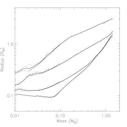
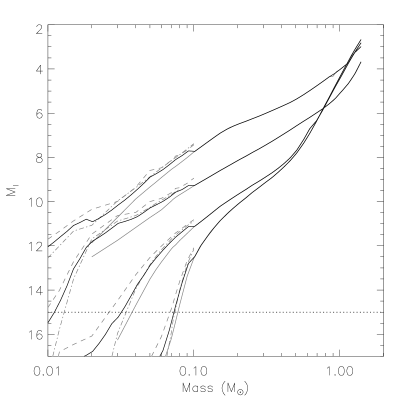
Figure 4: Mass-radius (left) and mass-absolute $I$-band magnitude (right) relations used in the calculations, shown here for 1, 10, 100 and 1000 Myr (from top to bottom). The model isochrones of Baraffe et al. (1998); Chabrier et al. (2000) and Baraffe et al. (2003) are shown in grey (solid, dash-dot and dashed lines respectively) and the adopted relation in black. The horizontal dotted line in the right-hand panel shows the faint limit of our observations ($I\sim 19$) in the closest of our target clusters (Blanco 1, $(M-m)_{0}\sim 7$).

To estimate the radius and absolute $I$-band magnitudes of stars and brown dwarfs of a given mass, we interpolate over tabulated relations between mass, radius and absolute magnitude which are illustrated for selected ages in Figure 4. The adopted relations at each age were obtained by combining the NEXTGEN isochrones of Baraffe et al. (1998), the DUSTY isochrones of Chabrier et al. (2000), and the COND isochrones of Baraffe et al. (2003), which span a total mass range $0.5\,M_{\rm J}$ to $1.4\,M_{\sun}$, taking the mean of the values predicted by the different models in the mass ranges of overlap. The apparent $I$-band magnitude is then deduced from the absolute magnitude using published values for the cluster distance $d$ and reddening $E(B-V)$, using the extinction law of Binney & Merrifield (1998).

Although the DUSTY and COND models diverge strongly at low masses, this occurs for very faint absolute magnitudes. As our deepest observations reach no fainter than $I\sim 22$ and the closest target cluster (Blanco 1) has $(M-m)_{0}\sim 7$, no detections are expected for primaries with $M_{I}>15$ (dotted line in Figure 4). Therefore, our very crude approach of taking the average of the different models even where they diverge should not strongly affect the results of the calculations. However, one should bear in mind that the mass-radius and mass-magnitude relations used in the present work are indicative only, especially given the intrinsic model uncertainties discussed in Sections 1.1 and 1.2.

3.4.2 Behaviour of $P_{\rm o}$

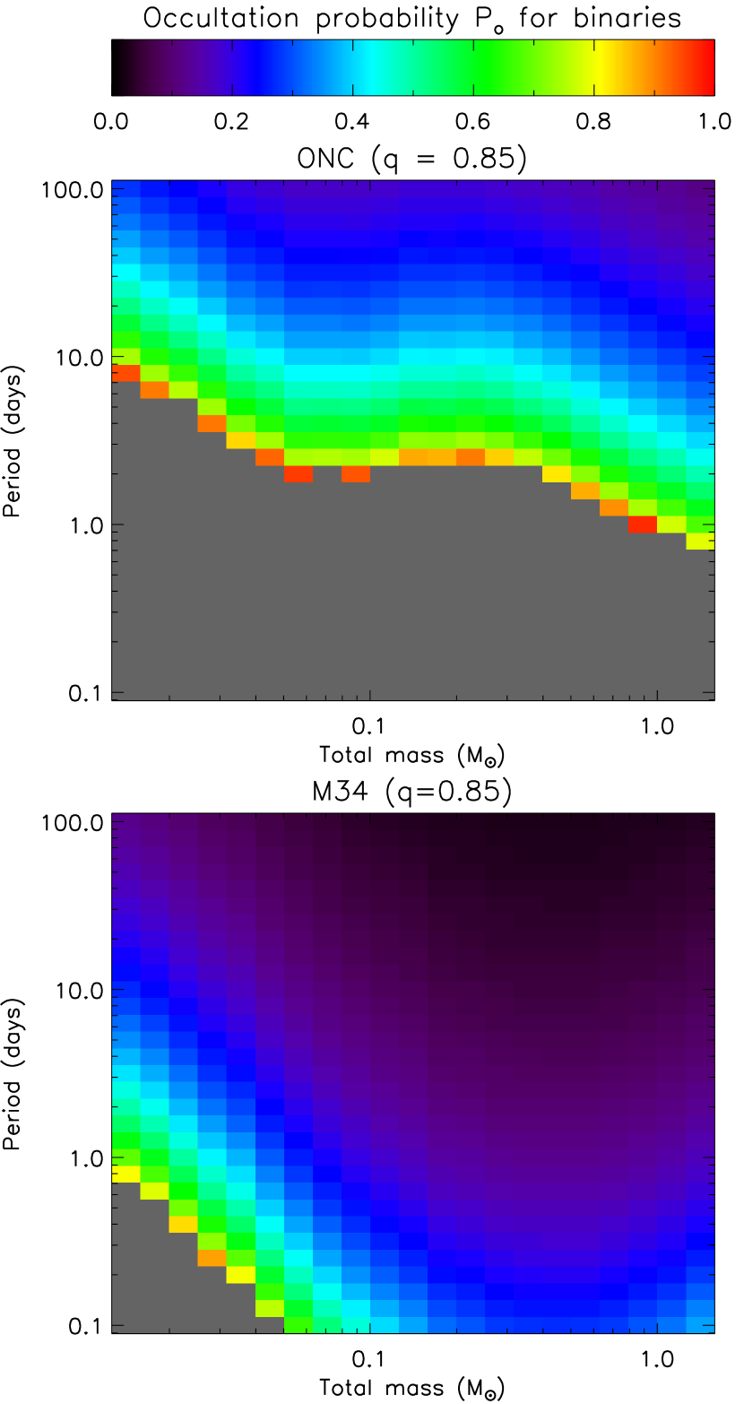
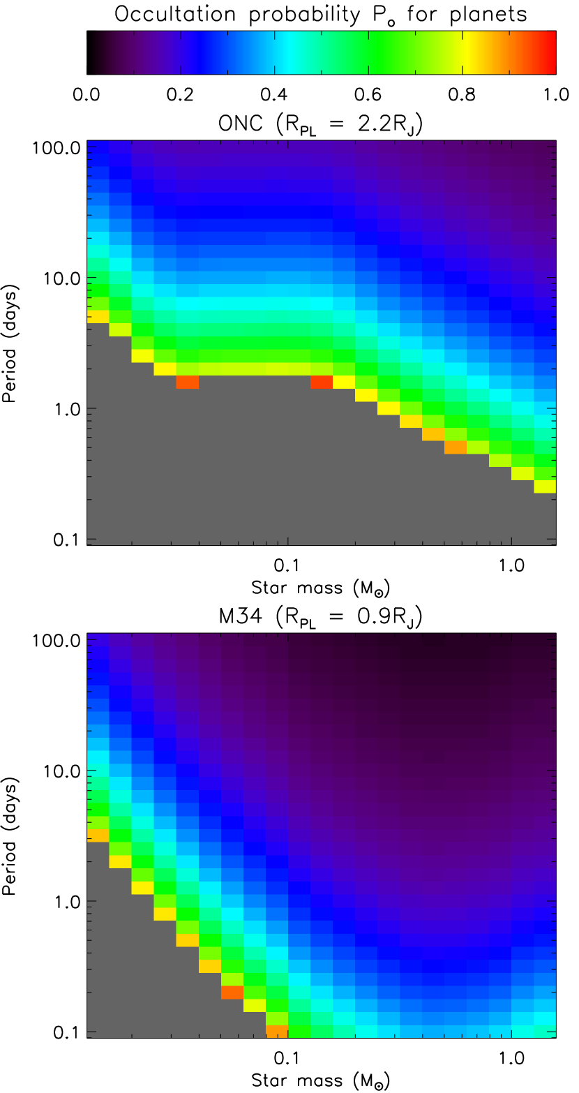
Figure 5: Example two-dimensional cuts through the three-dimensional occultation probability for the ONC (1 Myr, top) and M34 (200 Myr, bottom), for eclipses with mass ratio $q=0.85$ (left) and transits (right), for planet radii of $2.2\,R_{\rm Jup}$ (top) and $0.9\,R_{\rm Jup}$ (bottom). Regions shown in grey correspond to systems with orbital distance $a\leq R$.

Having adopted a mass-radius relation, we are now in a position to compute occultation probabilities for binaries, i.e. eclipse probabilities. To do this, $M_{1}$ and $M_{2}$ are deduced from $M$ and $q$, the mass-radius relation is used to give $R_{1}$ and $R_{2}$, which are summed to give $R$. For planets, computing transit probabilities involves deducing $M_{1}$ directly from $M$ (as all planets are assumed to have mass $M_{\rm Jup}$), applying the mass-radius relation to give $R_{1}$, and adding it to $R_{2}$ to give $R$. In both cases, $R$ is then inserted back into Equation (12) to give $P_{\rm o}$. Figure 5 shows 2–D cuts through the 3–D occultation probability for two example clusters. Close inspection of this figure highlights a few interesting points.

First, significant ($>0.2$) occultation probabilities are encountered throughout much of the parameter space of interest, even for planets (though this is no longer true for planets with radii much below that of Jupiter). This is due to the relative youth and low masses of the systems. As shown on Figure 4, young stars are larger than their main sequence counterparts, while Kepler’s $3^{\rm rd}$ law implies that low-mass systems have smaller orbital distances – for the same period – as their higher mass counterparts. Both of these effects tend to increase occultation probabilities.

Equation (12) also implies that, for a given total mass and period, the occultation probability (and duration) increases towards lower companion masses throughout the range of companions for which the mass-radius relation is relatively flat (up to $\sim 0.1\,M_{\sun}$ at 1 Gyr). As the occultation depths will also be comparable, this means that – from the point of view of occultation detection alone, and ignoring the incidence of such systems and the constraints imposed by the need to perform RV follow-up – we should be at least as sensitive to transits as to eclipses in that regime.

Third, alignment considerations favour short period, low-mass systems. These are particularly interesting because they offer very stringent constraints for star formation theories. Finally, the parameter space explored could nominally contain contact and over-contact systems – though the existence of such systems at such early ages is far from established. This will need to be kept in mind when modeling light curves in detail. For now, we set $P_{\rm o}=0$ for systems with $a\leq 2R$, to avoid counting these systems in the overall detection rate estimates.

3.5 Detection probability $P_{\rm d}$

The detection probability is evaluated using a Monte Carlo approach. For each of $N_{\rm sim}$ realisations, we randomly select an epoch and an inclination for the systems. Both the epoch and the cosine of the inclination are drawn from a uniform distribution, the latter being restricted to the the range $\cos i_{\rm min}\leq\cos i\leq 1$ for which occultations occur, where $\cos i_{\rm min}$ is directly deduced from $P_{\rm o}$:

$$\cos i_{\rm min}=\frac{R}{a}=P_{\rm o}$$ (13)

For each realisation we evaluate whether the occultations would have been detectable given the time sequence and noise properties of the data. $P_{\rm d}$ is then the fraction of the number of realisations in which the occultations would have been detectable.

3.5.1 Detection statistic

To evaluate the detectability of a given set of occultations, we compute the detection statistic that it would give rise to, assuming that a least-squares double-trapezoid fitting algorithm will be used for detection.

Among the most successful tools to search for occultations to date are algorithms based on least-squares fitting of box-shaped transits (Kovács et al., 2002; Aigrain & Irwin, 2004). In such algorithms, the detection statistic to maximise is often defined as the ‘signal-to-noise’ $S$ of the transit, which is the square-root of the difference in reduced chi-squared, $\Delta\chi^{2}$, between a constant model and the box-shaped transit model:

$$S^{2}=\Delta\chi^{2}=\frac{\delta^{2}}{\sigma_{\rm w}^{2}/n_{\rm t}}$$ (14)

where $\delta$ is the transit depth, $\sigma_{\rm w}$ is the white noise level per data point (assumed here to be the same for all data points) and $n_{\rm t}$ is the number in-transit data points.

However, the true properties of the noise on occultation timescales are generally not white. Pont et al. (2006) have recently examined how correlated noise on timescales of a few hours affects the detectability of planetary transits, and proposed a modification of this expression to account for correlated noise over a transit timescale:

$$S^{2}=\Delta\chi^{2}=\frac{\delta^{2}}{\sigma_{\rm w}^{2}/n_{\rm t}+\sigma_{\rm r}^{2}/N_{\rm t}}$$ (15)

where $\sigma_{\rm r}$ is the correlated noise over the transit duration, and $N_{\rm t}$ is the number of distinct transits sampled.

Box-shaped transit-finding algorithms were designed with shallow planetary transits in mind, whereas the majority of the occultations expected in the context of the Monitor project will be deep and grazing. A double-trapezoid occultation model, of which a single box-shaped transit is a special case, will provide improved detection performance (one can show that a box-shaped transit-search tool will recover 94% of the signal from a single triangular occultation, Aigrain 2005), and significantly better parameter estimation. Such an algorithm will be described in more detail in Aigrain, Mazeh & Tamuz (in prep.). The detection statistic for such an algorithm is defined as:

$$S^{2}=\Delta\chi^{2}=\frac{\delta_{1}^{2}}{\sigma_{\rm w}^{2}/\Sigma_{1}+\sigma_{\rm r}^{2}/N_{{\rm t},1}}+\frac{\delta_{2}^{2}}{\sigma_{\rm w}^{2}/\Sigma_{2}+\sigma_{\rm r}^{2}/N_{{\rm t},2}}$$ (16)

where $\delta_{1}$ ($\delta_{2}$) is the maximum depth of the primary (secondary) occultation, $N_{{\rm t},1}$ ($N_{{\rm t},2}$) is the number of distinct primary (secondary) occultations sampled, and $\Sigma_{1}$ ($\Sigma_{2}$) is the sum of the weights attributed to the data points in the primary (secondary) occultation. This sum is given by

$$\Sigma_{x}=n_{\rm c}+\sum\frac{2\left(\tau_{i}-d_{1}/2\right)}{d_{2}-d_{1}}$$ (17)

where $n_{\rm c}$ is the number of points falling the central (flat) part of the occultations, the summation runs over the remaining in-occultation data points (which fall in the egress or egress) and $\tau_{i}$ is the absolute deviation of the time of observation $i$ from the centre of the occultation.

Pont et al. (2006) find that a value of $S_{\rm lim}\sim 8$ is suitable for typical survey parameters to define the level at which the false alarm rate becomes unacceptably high. However, two additional requirements were imposed. The first is that at least two distinct occultations be sampled, which gives an upper limit to the orbital period. The second is that a minimum of 4 in-occultation points be observed in total, so as to provide a minimum of information on the shape of the event. Note that Aigrain & Favata (2002) found that 4 in-transit bins provide the best performance when using a step-function model with a variable number of in-transit bins for detection purposes, which indicates that 4 samples adequately describe the event (although in the present case, there is no guarantee that the samples are evenly spaced within the occultation).

3.5.2 Occultation parameters

In magnitude units, and if one ignores limb-darkening (recalling that most Monitor data is obtained in $I$- or $i$-band where limb-darkening is weak), occultations can be approximated as trapezoids with a linear ingress, an optional flat-bottomed section, and a linear egress. The occultation internal and external durations $d_{1}$ and $d_{2}$ are computed analytically assuming circular orbits (see e.g. Seager & Mallén-Ornelas, 2003):

$$d_{1}=\frac{p}{\pi}\,\arcsin\left[\frac{1}{a\,\sin i}\sqrt{\left(R_{1}+R_{2}\right)^{2}-\left(a\,\cos i\right)^{2}}\right]$$ (18)

$$d_{2}=\frac{p}{\pi}\,\arcsin\left[\frac{1}{a\,\sin i}\sqrt{\left(|R_{1}-R_{2}|\right)^{2}-\left(a\,\cos i\right)^{2}}\right].$$ (19)

The occultation depths are evaluated numerically by constructing a pixelised image of the disk of each component, with zero pixel values outside the disk. The fraction of one disk hidden behind the other at the centre of each occultation is evaluated by taking the pixel-by-pixel product of the two images, appropriately positioned relative to each other, and totaling up the number of non-zero pixels in the result. The in-occultation flux is then obtained by subtracting from the total out-of-occultation flux (the sum of disk-integrated fluxes from both component) the fraction of the occulted star’s flux that is hidden from view. Again, limb-darkening is not taken into account.

3.5.3 Noise level

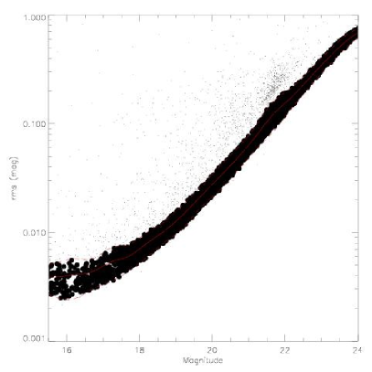
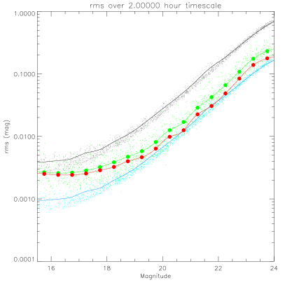
Figure 6: Left: Frame-to-frame rms $\sigma_{\rm w}$ versus magnitude for all M50 observations. Small black dots: all objects with stellar morphological classifications. Solid red line: spline fit to median rms versus magnitude. Dashed red lines: limits of the selection region for non-variable stars. Large black dots: objects selected as non-variable. Right: Noise budget over a 2 h timescale. Small black dots: frame-to-frame rms for 100 non-variable objects per 0.5 mag bin, selected at random. Black line: spline fit to median frame-to-frame rms versus magnitude. Blue dots and line: idem, divided by $\sqrt{n_{\rm int}}$. Green small dots, large dots and line: scatter $\sigma_{\rm s}$ of individual light curves over 2 h times, median value in each magnitude bin, and fit thereto. Red small dots, large dots and line: idem for $\sigma_{\rm r}$.

We compute the noise budget of the light curves from our existing data. The white and red noise levels $\sigma_{\rm w}$ and $\sigma_{\rm r}$ are both magnitude dependent, the latter also depending on the occultation duration. Therefore, $\sigma_{\rm w}$ is evaluated once per cluster, based on the median of the noise levels of the non variable stars, and $\sigma_{\rm r}$ is evaluated once per cluster for a range of likely occultation durations (from 0.5 to 3.5 h)

First, we compute the median and scatter in each light curve (using robust median-based estimators). We then sort the light curves into 0.5 mag wide bins of median magnitude, and compute the median $\sigma_{\rm w}$ and scatter of the frame-to-frame rms in each bin. A spline is then fitted to each quantity, and stars whose $\sigma_{\rm w}$ fall within one sigma of the median rms fit are selected as “non variables”.

In each magnitude bin, we then select 100 non variable light curves at random and use these to evaluate the average noise properties in that bin. Each light curve is then smoothed over a number of timescales $d$ ranging from 30 min to 3.5 h, and we record the scatter $\sigma_{\rm s}$ of the smoothed light curve, counting only the intervals where the smoothing window did not overlap with any data gaps. If a light curve was affected by white noise only, we would expect $\sigma_{\rm s}=\sigma_{\rm w}\,n_{\rm int}^{-1/2}$, where $n_{\rm int}=d/\delta t$ and $\delta t$ is the average interval between consecutive data points. In general, $\sigma_{\rm s}$ is higher, owing to correlated, or red, noise. For each bin, the average of the $\sigma_{\rm s}$ of all 100 selected light curves is modeled as the quadrature sum of a red and white noise components: $\sigma^{2}_{\rm r}=\sigma^{2}_{\rm s}-\sigma^{2}_{\rm w}/n_{\rm int}$. The results of this procedure are shown for M50 and $d=2$ h in Figure 6.

For each total system mass and, for binaries, mass ratio, the total system magnitude is evaluated as follows. Applying the mass-magnitude relation at the appropriate age to $M_{1}$ and $M_{2}$ and correcting for the cluster distance and reddening, yields apparent $I$-band magnitudes $I_{1}$ and $I_{2}$. The total system magnitude is then $I=-2.5\log\left(10^{-0.4I_{1}}+10^{-0.4I_{2}}\right)$. If $I<I_{\rm sat}$ or $I>I_{\rm sat}$, we set $P_{\rm d}=0$, to avoid counting saturated systems or wasting time computing $P_{\rm d}$ for systems which are not monitored sufficiently precisely to give a useful measurement of the occultation depth. In all other cases, interpolating over spline fits to the relations between magnitude and frame-to-frame and red noise (over the most appropriate timescale, i.e. that closest to $d_{1}$) yields the relevant values of $\sigma_{\rm w}$ and $\sigma_{\rm r}$, which can then be inserted into into Equation (16).

3.5.4 Behaviour of $P_{\rm d}$

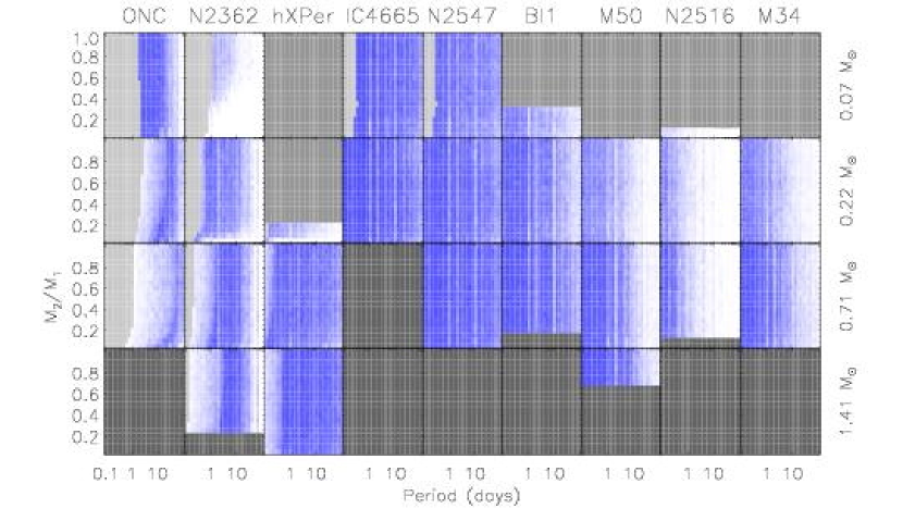
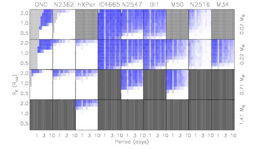
Figure 7: Diagrams of $P_{\rm d}$ for binaries (top) and planets (bottom), as a function of orbital period (x-axis) and mass ratio or planet radius (y-axis) for each cluster (columns) and selected total system masses (rows). Blue areas correspond to detection probabilities close to 1 and the colour scale is linear. Areas shaded in light grey correspond to contact systems. Areas shaded in medium and dark grey correspond to systems that are too faint or saturated respectively.

The detection probabilities $P_{\rm d}$, computed as described above, are illustrated for all the clusters in Figure 7. They are shown as a function of period and companion mass (eclipses) or radius (transits) for a variety of total system masses. These diagrams give a broad overview of the sensitivity of our survey over the full parameter space.

At the time of writing, the photometric monitoring observations are complete for three of our target clusters only. For all the other cases, we used data from clusters observed in similar conditions to estimate the noise properties, and added to or generated the time sequence of observations artificially, ensuring the simulated time sequence matches what is expected at least in the statistical sense. Note that although we do have data from our INT campaign on the ONC, we estimated the photometric precision based on observations of M34 with the same telescope, because the intrinsic variability of ONC stars makes it difficult to evaluate the true noise level from the ONC light curves themselves. We used both the noise properties and the time sequence of our CTIO campaign in NGC 2516 to evaluate the sensitivity of our KPNO survey in M34 and $h$ & $\chi$ Per, as the telescopes and instruments are twins of each other and the observing strategies closely matched. Wherever a given cluster was observed with more than one telescope (m34, $h$ & $\chi$  Per), the simulations were carried out separately for each telescope. Figure 7 then shows, for each total mass, mass ratio or radius and period bin, the highest of the sensitivities achieved with the different telescopes.

In each cluster, the survey was designed to ensure good sensitivity to eclipses, and the sensitivity diagrams reflect this, with very good sensitivity throughout much of the parameter space of interest for binaries. Provided the period is short enough to accumulate the minimum required number of observed in-transit points and transit events, the eclipses of systems of all mass ratios are generally easily detectable. It is only for the lowest total system masses that mass ratio affects the sensitivity. For a given total mass, lower mass ratio systems correspond to more massive (hence brighter) primaries, counterbalancing the decrease in eclipse depth. When considering the columns corresponding to $h$ & $\chi$ Per and M34, one should keep in mind that the results shown are the combined results for several surveys with different telescopes and observing strategies, which leads to some discontinuities in the overall sensitivities.

In the clusters observed exclusively in visitor mode, we are sensitive only to very short periods. As the eclipses are often deep and even a single in-eclipse point can be highly significant, this short-period bias is a consequence of the requirement that at least two separate transit events be observed, rather than a direct detection limit. The advantage of repeating observations after an interval of at least several months is visible in the columns corresponding to the ONC, NGC 2362 and M50, where the sensitivity remains good up to $\sim 10$ days. The clusters observed in snapshot mode benefit from increased sensitivity at long periods. However one should keep in mind that we have not analysed data from any snapshot mode observations to date. Snapshot mode observations may be affected by long-term stability issues which will be hard to calibrate with the very patchy time coverage we foresee. The performance of this mode compared to more traditional visitor mode observations therefore remains to be confirmed. In all cases, the complex period dependence of the sensitivity is not fully resolved in the rather coarse grid we used, but some of the ubiquitous sensitivity dips at exact multiples of 1 day, which are typical of transit surveys (Pont et al., 2005; Gaudi et al., 2005), are clearly visible. Because of the relatively coarse logarithmic period sampling used, these dips are visible at 1, 2 and 10 day, where the injected period was exactly a multiple of a day, but in reality they would be present at all exact multiples of 1 day.

As expected, sensitivity to transits is much lower. The minimum detectable planet radius is essentially a function of the cluster age (which affects the stellar radii – see ONC) and distance (which affects the photometric precision – see NGC 2362 and $h$ & $\chi$ Per). The importance of accumulating enough data is highlighted by the very poor sensitivity in clusters observed for less than the required 100 h (NGC 2516 and M34 at the high-mass end). It is interesting to note that we are particularly sensitive to transits around low-mass stars. We are limited to radii above that of Jupiter in the youngest clusters, but this ties in with the expectation that planets as well as stars are bloated at early ages. The sensitivity peaks around M-stars, where planets with radii significantly below that of Jupiter are detectable in some cases.

3.6 Results

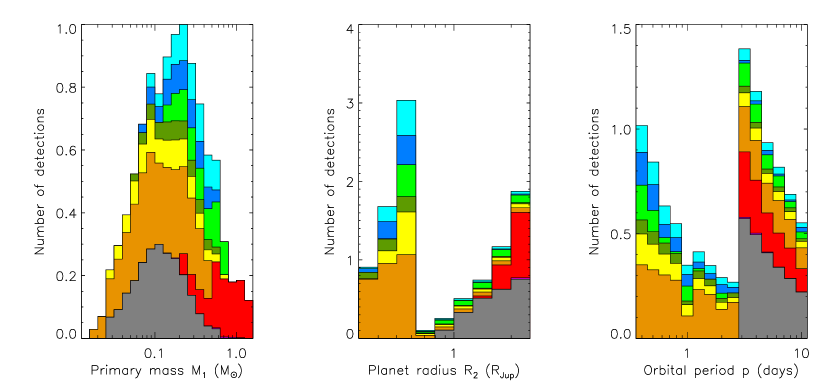
Figure 8: Number of expected detections for binaries (top) as a function of primary mass (left), mass ratio (centre) and orbital period (right), and for planets (bottom) as a function of primary mass (left), planet radius (centre) and orbital period (right). The histograms are summed, each of the cluster being represented by a different colour, starting with the youngest (the ONC, in grey) at the bottom and ending with the oldest (M34, in light blue) at the top. The overall filled area corresponds to the total number of detections, all clusters combined.

	Binaries			Planets
Name	$N_{\rm c}$	$N_{\rm o}$	$N_{\rm d}$	$N_{\rm c}$	$N_{\rm o}$	$N_{\rm d}$
ONC	167.3	57.3	27.8	135.0	47.8	2.3
NGC 2362	45.6	11.0	4.7	37.1	11.3	0.0
$h$ & $\chi$ Per	648.9	106.0	67.0	631.9	118.1	1.2
IC 4665	21.5	5.8	4.6	14.3	4.3	3.1
NGC 2547	30.4	5.1	3.9	20.7	3.9	0.9
Blanco 1	10.3	0.9	0.6	8.0	1.0	0.5
M50	160.0	12.7	5.4	127.0	13.4	0.8
NGC 2516	103.0	8.4	1.5	76.9	8.4	0.7
M34	45.1	3.4	1.4	34.1	3.5	0.8
Total	1230.7	207.3	114.0	1084.4	209.4	8.6

Table 4: Expected number of binaries, eclipsing binaries and detectable eclipsing binaries, and of planets, transiting planets and detectable transiting planets, for each cluster and for the survey as a whole, under the assumptions described in the text.

Table 4 shows the number of observed cluster members with companions, the number of observed occulting systems and the number of detectable occulting systems for each cluster, for binaries and planets separately. The former two are given by

$$N_{\rm c}=\int\int\int N_{\rm sys}P_{\rm c}~{}{\mathrm{d}}\log M~{}{\mathrm{d}}x~{}{\mathrm{d}}P$$ (20)

and

$$N_{\rm o}=\int\int\int N_{\rm sys}P_{\rm c}P_{\rm o}~{}{\mathrm{d}}\log M~{}{\mathrm{d}}x~{}{\mathrm{d}}P$$ (21)

where the integrals are performed on the entire range of parameter space in the simulations, ignoring saturated or excessively faint systems. The distribution of the detections in each cluster in terms of primary mass, mass ratio (or planet radius) and orbital period is shown in Figure 8.

For the binaries, the main limiting factor is the number of systems surveyed, which implies that the number of detections expected in some clusters (e.g. Blanco 1, NGC 2516, M34) is of order unity, despite good sensitivity ($P_{\rm d}$ close to 1 over much of the parameter space of interest). Given that each detection places a useful constraint on a currently ill-constrained region of the mass-radius relation, even those small numbers are interesting. On the other hand, the number of expected detections in the rich twin clusters $h$ & $\chi$ Per is very large, despite the fact that we are only sensitive to companions to relatively massive stars. In the other clusters, and a fortiori for Monitor as a whole, significant numbers of detections are expected. These should provide not only strong constraints on the mass-radius relation over a range of masses, but also imply that the Monitor survey will enable us to test hypotheses regarding the binary fraction of low-mass stars at early ages and the distributions of mass ratios and orbital periods for young binaries.

Figure 8 reflects the combination of the mass function of each cluster, our assumptions about companion incidence and the detection biases, mainly visible as a downward slope in the period distribution. In the top row, corresponding to binaries, we see two main types of behaviour. For the youngest clusters (the ONC and NGC 2362), we are sensitive primarily to low mass systems. The mass ratio distribution is consequentially dominated by the peak around $q=1$, with very few low mass ratio systems. We predict few detections with $p<1$ d because these are contact systems at such early ages. For the rest of the clusters, we have a more mixed picture, including systems on both sides of the $M=0.5\,M_{\sun}$ boundary, and our observations should thus enable us to test the hypotheses we have made about the dependence of the mass ratio and period distributions on total system mass (or primary mass).

We expect of order one planetary transit to be detected per cluster. While this may seem like a low number, it is relatively high compared to the amount of telescope time invested for a transit survey, specially bearing in mind the particularly high potential scientific impact of a transit detection in a young cluster.

As in the binary regime, there is also a clear distinction between the youngest clusters (this time including $h$ & $\chi$ Per as well as the ONC) and the older ones in the planet regime. As shown in the bottom row of Figure 8, in the ONC, we probe mainly the Hot Jupiter population around low-mass stars, and we should be able to test how much it differs from that around higher mass stars and at later ages. The large size of the stars excluding both shorter period systems (because of contact issues), and smaller planets (because the transits are too shallow). No detections are expected in NGC 2362 because it suffers from the same star-size issue as the ONC, but the low-mass stars are too faint to allow us to detect Hot Jupiters around them. In $h$ & $\chi$ Per, the large number of targets somewhat compensates the large cluster distance to give a relatively high number of detections, and we are mainly sampling the Hot Jupiter population around Sun-like stars, enabling a direct comparison to the same population already well studied around older field stars. Together, the ONC and $h$ & $\chi$ Per constitute a very populous (nearly 10 000 targets) and interesting test-bed of planet formation timescales, spanning as they do the full range of circumstellar disk lifetimes. If no transits are detected in the ONC or $h$ & $\chi$ Per, this will place a very strong upper limit on the incidence of close-in giant planets at early ages.

On the other hand, for the older clusters, the majority of the detections are expected in the very Hot Neptune regime. This is because we have assumed, in a rather ad hoc fashion, that very Hot Neptunes are relatively common, whereas we have assumed, based on observational evidence to date, that very Hot Jupiters are much rarer. If very Hot Jupiters were more common than we have assumed, we would detect them too. What Figure 8 really implies is that, in the older clusters, we are almost exclusively sensitive to the very Hot ($p<3$ d) planet population, as are most other transit surveys whether in the field or in clusters, but we are sensitive to relatively small planets – as noted by Pepper & Gaudi (2005b). If very Hot Neptunes are significantly rarer than we have assumed, we could easily have no detections in any of this older group of clusters. Under the set of assumptions used here, however, it is in IC 4665 that the largest number of transit detections of all the target clusters is expected, despite the relatively low density of clsuter members, because the host-star mass range we monitor are very favourable for a transit survey. In this cluster, we are primarily sensitive to very short period planets around very low-mass stars and brown dwarfs, and this cluster will thus provide an interesting test of the abundance of this type of planet.

In all clusters, the distribution of primary masses reflects mainly the mass function of the cluster within the survey limits, and the assumed difference in planet incidence between primaries above and below $0.5\,_{\sun}$ is relatively hard to see except for $h$ & $\chi$ Per.

4 Spectroscopic follow-up

4.1 Strategy

The light curve alone is not sufficient to ascertain the nature of any companions detected through their occultations. Even if one assumes that the primary lies on the cluster sequence, and that its mass and radius are known, the light curve provides only an estimate of the companion radius. Of course, photometrically selected candidates may not in fact be cluster members. In addition, even if they are members, the mass-radius-luminosity relations are so uncertain at early ages and low masses that any photometric estimates of the primary mass and radius could be highly unreliable. This last point is most valid for the ONC, because of its youth, age spread, differential reddening and the particularly low primary masses to which we are sensitive.

Multi-epoch spectroscopy is thus needed to ascertain the cluster membership of any candidate systems and to determine the masses of the components through radial velocity (RV) measurements. The relatively faint nature of the target stars means that high-resolution spectroscopy is extremely time consuming, and we have therefore opted for a two-step follow-up strategy, consisting of at least one medium resolution spectrum ($R\sim 5000$ to $10\,000$) on 2 to 4 m class telescopes, followed by multiple high resolution spectra ($R\sim 40\,000$) on 6 to 8 m class telescopes for those candidates that warrant it.

The number of RV epochs needed to constrain the companion mass is minimised if a precise ephemeris for the occultations is available. This requires several ($\geq 3$) occultations to have been observed, and – unless the spectroscopic follow-up is carried out in the same season as the original photometric survey – occultations observed in more than one season. For good candidates which do not fulfill these criteria, we therefore foresee a photometric follow-up stage, using telescopes with flexible scheduling and modest field-of-view detectors, to attempt to observe additional eclipses. This photometric follow-up can take place in the same time frame as the first stage spectroscopic follow-up, as long as the refined ephemeris is available when the RV data are analysed. These observations are also used to attempt to detect secondary occultations when the phase coverage of the initial observations did not allow it. If carried out in multiple bandpasses, they can also be used to refine the determination of the fundamental parameters of the components.

Three main types of contaminants are foreseen:

• Background giants. In the case of most of our target clusters, any background giants would have to be outside the Galaxy to pass our membership cut. This is therefore not a major source of contamination, though medium-resolution spectroscopy allows the identification for most late-type giants through the measurement of gravity sensitivity features;

• Background field dwarfs reddened onto the cluster sequence. These constitute the main source of contamination, but can be weeded out by comparing their spectral type to that expected from their optical and near-IR colours, because they do not follow the same colour-spectral type relation as cluster members;

• Unreddened field stars which do follow a similar colour-spectral type relation to cluster members, but which lie in range of apparent magnitudes which allows them to pass our membership cut. This implies that they must lie in a rather restricted volume, mostly on the near-side of the cluster, and the number of contaminants of this type is not expected to be very large. A lack of youth indicators such as Lithium absorption lines and H$\alpha$ emission in the spectrum will be the main way of identifying these objects, together with dynamical indicators (systemic radial velocity incompatible with that of the cluster).

A single medium resolution spectrum in the red part of the visible with a signal to noise ratio better than 20 per resolution element typically requires less than 1 h of exposure for a target with $I<18.5$ on a 4 m telescope, and yields spectral classification to better than one subclass (based on Kirkpatrick et al. (1991) relative flux indices). This is complemented by the search for youth indicators (H$\alpha$ emission, Lithium absorption), though these are expected to be present in some of our targets only. Gravity sensitive lines and indices also provide some degree of discrimination between young cluster members and giants or old field dwarfs.

This initial spectrum also typically provides a first epoch radial velocity measurement at the few km/s level, which should suffice to detect the variations induced by any stellar and most brown dwarf companions (a $0.03\,M\,_{\sun}$ BD in a $10$ d orbit around a solar mass star will induce an RV amplitude of $3$ km/s in the primary, and shorter periods or larger mass ratio lead to increased amplitudes). Unless the object has clearly been identified as a non-member from the first spectrum, a small number of additional medium resolution spectra are taken. If no RV variations are detected at the km/s level, the object remains a good candidate provided the depth of the occultations is consistent with a very low-mass companion (otherwise, one must question the true nature of the occultations). If variations are detected, they can be used to measure – or at least place a lower limit on – the RV amplitude of the primary, and thus the mass ratio of the system. Whether variations are detected or not, this first set of measurements also provides an estimate of the systemic radial velocity. Comparison of this with the cluster radial velocity provides an independent test of cluster membership.

High resolution spectroscopy is then needed for all candidates that survive the previous stage, i.e. those for which we derive a spectral type and systemic RV consistent with cluster membership, and where either we detect RV modulations, or the non-detection of RV modulations is consistent with the minimum companion mass implied by the light curve and our estimate of the primary mass, given the RV precision achieved with medium resolution spectra. In cases where we have detected RV modulations, the goal of this second stage is to resolve the secondary set of lines, and to obtain a full orbital solution. In this case, the observations are best carried out in the near-infrared (with instruments such as Phoenix on Gemini or CRIRES at the VLT), where the contrast between primary and secondary is lower than in the visible.

In cases where no RV modulation was detected so far, the second set of lines is unlikely to be detectable, but increased RV precision is needed to resolve the very low amplitude modulations of the primary. For those systems, estimates of the mass and radius of the primary must rely on relations between effective temperature (deduced from the spectrum), mass and radius which, as we have seen in Section 1, are very poorly calibrated at early ages. If high mass ratio systems are detected in the same cluster as low mass ratio systems, the constraints the former will provide on these relations will be used to refine the estimates of the parameters of the primaries of the latter.

In the Section 4.2, we investigate the expected RV precision as a function of magnitude and rotational velocity with medium resolution instruments on 4m class telescopes (such as EMMI on the NTT or ISIS on the WHT) and with higher resolution instruments on 8m class telescopes (such as FLAMES and UVES on the VLT).

4.2 Limits imposed by radial velocity accuracy

Although the flux from both primary and secondary is maximised in the near IR for low mass stars, precision RV work from near-IR spectra is a relatively un-tested area. On the other hand, recent surveys in the optical have generated a wealth of information on the achievable RV performance. An additional advantage of the optical is the availability of high resolution spectrographs with wide-field multiplexing capabilities. Therefore, we investigate here the optical only.

State of the art RV instruments are today reaching accuracies of a few m/s, and are capable of detecting the modulations imparted on their parent stars even by Neptune-mass planets (see e.g. Lovis et al., 2006). However, this requires multiple, very high resolution spectra to be obtained with relatively high signal-to-noise ratio, and is hence feasible only for bright stars. Candidates from transit surveys carried out on telescopes with apertures of 1 m and above tend to be much fainter, which makes their follow-up much more difficult. However, the recent campaigns to follow-up OGLE candidates (Bouchy et al., 2005; Pont et al., 2005) have shown that it is possible to obtain reach RV accuracies down to $\sim 100$ m/s down to $I=17$ for non-rotating stars with FLAMES on the VLT, using high resolution spectra ($R~{}20\,000$–$40\,000$) covering a broad wavelength range centred on $\sim 600$ nm, with a simultaneous ThAr reference for wavelength calibration.

Many of the candidates expected in the context of Monitor are both fainter and much redder than OGLE targets. Using a redder part of the spectrum allows useful signal-to-noise ratios to be accumulated in much shorter exposure times, at the cost of a smaller number of lines and the loss of the simultaneous wavelength reference. In particular, the Ca ii triplet around 850 nm (hereafter Ca T) is routinely used for stellar population kinematic studies, yielding accuracies down to 2 km/s in reasonable exposure times down to $I\sim 18$ using FORS on the VLT (see e.g. Pont et al., 2004).

We have therefore computed the limiting RV accuracy achievable in 1 h exposure times as a function of magnitude and projected rotation rate $v\sin i$ (rotation broadens the lines and limits the achievable accuracy for three types of observations):

• Ca T observations using medium resolution spectrographs on 4 m class telescopes, such as EMMI on the NTT or ISIS on the WHT (hereafter M850);

• Ca T observations using higher resolution spectrographs on 8 m class telescopes, such as FLAMES on the VLT (hereafter H850);

• observations in the 600 nm region using higher resolution spectrographs on 8 m class telescopes, such as FLAMES on the VLT (hereafter H600).

The M850 calculations enable us to check what fraction of the objects for which we expect to detect eclipses we will detect the RV modulations for in the first (medium resolution) stage of our follow-up strategy (see Section 4.1). The detail of the calculations and settings used for each type of observations is given in Appendix A.

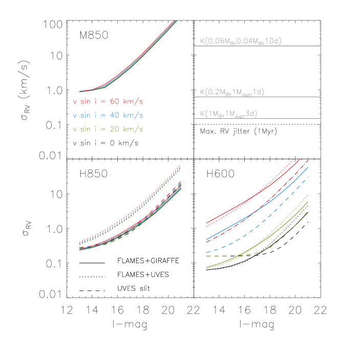
Figure 9: Theoretical radial velocity error as a function of apparent $I$-band magnitude based on M850, H850 and H600 observations (top left, bottom left and bottom right respectively). All calculations are based on integration times of up to 1 h taken in good atmospheric conditions (see text). The black, green, blue and red curves in each panel correspond to objects with $v\sin i$’s of 0, 20, 40 and 60 km/s respectively. In the top right panel, RV semi-amplitudes are shown as horizontal grey lines for the primaries of a number of example systems, labeled with the corresponding primary and secondary mass and orbital period. In the same panel, the black horizontal dotted line shows the activity induced RV jitter expected in the worst case (youngest, most active stars).

Figure 9 shows the results of this exercise for $v\sin i$ ranging from 0 to 60 km/s (i.e. rotation periods down to 0.8 days for a radius of $1\,R_{\sun}$). As expected, precisions of a few km/s can be achieved using M850 observations down to $I\sim 17$. The intrinsic width of the Ca T lines makes them very insensitive to rotation. To reach fainter objects or achieve better precision requires larger telescopes and higher resolution instruments. With those, still using the Ca T, i.e. H850, it is possible to reach precisions of $\sim 2$ km/s at $I\sim 18$ and $\sim 200$ m/s at $I\sim 13$, while H600 observations can provide increased precision – down to $\sim 50$ m/s at the bright end – provided the rotational velocity is moderate ($\leq 30$  km/s). These calculations assume an M2V spectral type and insignificant reddening.

This leads to the somewhat puzzling conclusion that neither spectral region is globally optimal, and that the optimal strategy will have to be selected on the basis of the spectral type and rotation periods or $v\sin i$ of the individual candidates (where those are not measured, rough estimates can be inferred from the candidate’s age and spectral type). The trade-off between the higher throughput of UVES in slit-mode and the lower seeing-induced errors of FLAMES will depend on the surface density of candidates in a given cluster. There appears to be little gain at any magnitude in using FLAMES$+$UVES over FLAMES$+$GIRAFFE.

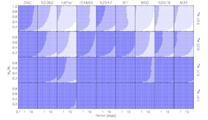
Figure 10: Estimated sensitivity to the RV modulations induced by stellar and substellar companions as a function of orbital period (x-axis) and mass ratio (y-axis) for each cluster (columns) and selected total system masses (rows). Dark, medium and light shading correspond to areas where M850, H850 and H600 observations respectively should allow us to detect the RV modulation.

The example RV semi amplitudes shown in the top right panel of Figure 9 show that we should be able to detect the RV modulation induced in the primary of most stellar and substellar binaries in our survey with medium resolution instruments, while a small fraction will require 8 m class follow-up. Only H600 observations of the brightest, slowly rotating stars allow the detection of planetary companions. This is illustrated on a cluster-by cluster basis in Figure 10, where we have shaded the areas of parameter space for which the RV modulations are detectable with each type of spectroscopic observations considered. We considered detectable any system where the RV semi amplitude $K$ is more than twice the estimated RV precision, i.e. well-timed observations should enable the detection of the RV modulation at the $4\sigma$ level. Comparison with Figure 7 highlights the good overlap between the photometric and RV sensitivity for binaries.

Table 5 shows, for each of the types of spectroscopic observations considered, the percentage of detected eclipses for which we also expect to detect the RV modulations. We have used the best case scenario, i.e. zero rotation and most appropriate instrument for the magnitude and rotation rate considered.

Table 5: Percentage of true eclipse / transit candidates with detectable radial velocity modulations. The letter a, b and c refer to the type of RV observations (see text). The last column gives the expected number of transiting planets whose RV modulation should be detectable in each cluster.

Name	Binaries			Planets
	a	b	c	c
	%	%	%	%	No.
ONC	84	100	100	100	2.3
NGC 2362	48	99	100	0	0.0
$h$ & $\chi$ Per	24	93	100	0	0.0
IC 4665	69	98	100	20	0.6
NGC 2547	76	100	100	28	0.3
Blanco 1	89	100	100	10	0.0
M50	48	98	100	10	0.1
NGC 2516	74	99	100	0	0.0
M34	59	98	100	0	0.0
Total	45	96	100	27	2.8

Except for $h$ & $\chi$ Per and M50, where we are primarily monitoring relatively massive primaries, the vast majority of the candidate eclipsing binaries will cause RV modulations detectable with M850 observations, i.e. after the first stage of our follow-up observation. Virtually all binary systems in all clusters that are detectable with photometry are also detectable in RV with H850 observations, and a fortiori with H600 observations. The numbers involved in $h$ & $\chi$ Per are so large that it is unrealistic to expect all of the candidates to be followed-up. Efficient follow-up of candidates in these twin clusters will require a Northern hemisphere high-resolution spectrograph with wide-field multiplexing capabilities such as WFMOS on SUBARU (Bassett et al., 2005).

For planets, H600 observations only have the potential to detect RV modulations. In the last two columns of Table 5, we give the percentage and number of transiting planets detected photometrically whose RV modulations should also be detectable with this type of observation, assuming a planet mass of $M_{\rm pl}=1\,M_{\rm Jup}$ for $M_{\rm pl}\geq 0.7\,M_{\rm Jup}$ and $M_{\rm pl}=0.3\,M_{\rm Jup}$ for $R_{\rm pl}<0.7\,R_{\rm Jup}$. For Jupiter-mass planets, the feasibility of RV follow-up is essentially dependent on the cluster distance, and as such will be particularly problematic in NGC 2362 (transit detection probabilities are also low in this cluster), $h$ & $\chi$ Per and M50, and to a lesser extent in M34. The majority of the Jupiter-mass planets causing detectable transits in the other clusters should induce RV modulations detectable with instruments such as UVES in the $V$-band, provided their parent stars are not rotating too fast (in particular, a significant fraction of planet host-stars in the ONC may be rapid rotators). The RV modulations induced by low-mass planets are very hard to detect in any of the target clusters. The complete end-to-end simulations predict around 3 confirmed detections overall, but one should bear in mind that this number may go up or down by a factor of two or more if one tunes the input assumptions within a reasonable range.

Table 6: Number of planetary systems detectable both via their transits and in radial velocity if every star with mass above $0.2\,M_{\sun}$ possesses a Jupiter mass companion in the range 0.4–10 d assuming a the ‘standard’ period distribution, i.e. 5 times as many Hot Jupiters as very Hot Jupiters (1), or a period distribution that is uniform in $\log P$ (2)..

Name	Number
	(1)	(2)
ONC	139.4	1917
NGC 2362	4.2	127
$h$ & $\chi$ Per	2.5	74
IC 4665	21.0	341
NGC 2547	15.4	299
Blanco 1	6.7	105
M50	6.1	183
NGC 2516	7.8	235
M34	6.8	203
Total	209.8	3482

It is interesting to examine the results under a different, highly optimistic set of assumptions regarding planetary companion incidence, to see whether Monitor will be able to place any kind of constraints on this incidence. Table 6 lists the number of confirmable detections expected if every star with mass above $0.2\,M_{\sun}$, hosts a Hot or very Hot Jupiter. This is by no means a realistic scenario: although the actual incidence of Hot and very Hot Jupiters may well be higher around very young stars than at later stages, for example if a ‘survival of the lucky few’ scenario applies, where most planets migrate into their parent stars and only those that form shortly before the disk disappears survive, this would at most imply a factor of a few increase in the incidence of planetary companions at early ages. However, it serves to illustrate that, if we do not detect planets in a given cluster, this will imply a strong upper limit on the incidence of close-in Jupiters in that cluster. Two possibilities for the period distribution were investigated, namely the same period distribution as used previsously, where Hot planets are five times more abundant than very Hot planets, and a distribution that is uniform in $\log P$. There is an increase by a factor $>10$ in the numbers for the second case, which illustrates the very strong bias of the detection method used (transits and radial velocities combined) towards short periods.

In practice, we will not know a priori which events are transits and which are eclipses. In cases where the occultation depth and duration in the initial light curve are consistent with a very low-mass occulting companion but no RV variations are detected, we will have to give careful consideration to what phenomena could mimic a planetary signal in our light curves without generating a detectable RV signal. Provided that cluster membership can be reliably assessed, a number of types of ‘difficult mimics’ remain: physical triple systems belonging to the cluster, starspots, and occultations by warps or accretion columns in nearly edge-on circumstellar disks. Simultaneous multi-band monitoring, including the full visible range and the near-IR, may help discriminate between these and planetary companions, but we cannot exclude the possibility that low mass brown dwarfs or planets whose transits we might detect will remain unconfirmed given the capabilities of present-day instrumentation. Even if every other hypothesis were excluded, detection of a planetary companion without a mass estimate would be of limited use in constraining formation and evolution models. We point out that these ‘unsolved systems’ will make interesting targets for extremely large telescopes (ELTs) foreseen to come into operation in the 2010–2020 period, such as the European ELT or the Thirty Meter Telescope (TMT), assuming they will be equipped with high resolution visible and near-IR spectroscopic instruments.

5 Conclusions and future prospects

We have undertaken a unprecedented survey whose primary goal is to search for occultations in all suitably young, nearby and rich young clusters with well-characterised pre-main sequence populations.

In this paper, we detailed the motivations for undertaking such a survey, highlighting the fact that occulting companions to young, low-mass stars constitute a critical area of parameter space, which has not been explored so far, and where each detection has the potential to act as a vital anchor point for formation and evolutionary models of low mass stars, brown dwarfs and planets.

After laying down the considerations which guided the design of the survey, many of which are dictated by availability of suitable instrumentation and other circumstances, rather than fully controlled, we have performed a detailed a priori assessment of the expected performance of the survey in each cluster and as a whole, incorporating the actual (observed) noise budget and time sampling of the observations wherever possible, and taking into account the limits imposed by the need to follow-up candidates spectroscopically as well as the detectability of occultations.

This has allowed us to explore which area of occulting systems parameter space we expect Monitor to be sensitive to, and what the limiting factors are. The range of total system masses which we observe with useful photometric precision depends on the cluster age and distance, the telescope aperture and the exposure time, but spans the entire low-mass star regime, from $1.4\,M_{\sun}$ to the Hydrogen burning mass limit (HBML), if one considers the entire target sample. We are primarily sensitive to short-period systems, but this bias is somewhat reduced by the fact that many occultations of interest are deep and hence clearly detectable even if a single event is observed (though a requirement that several events be observed was imposed when evaluating the detection rates).

Using a set of baseline assumptions for the incidence and parameter distribution of stellar and substellar companions, we have estimated the number of eclipsing binary systems that Monitor as a whole should detect. We find that Monitor should detect approximately 114 such systems. Close to half of the expected detections are in the twin clusters $h$ & $\chi$ Per, which our preliminary membership study confirms as extremely rich, and where we are mainly sensitive to total masses close to $1\,M_{\sun}$. The radial velocity modulations of these systems are detectable from 8 m class telescopes, though to follow-up all the expected candidates would require a very large allocation of telescope time. Monitor will thus have a very significant impact in constraining the multiplicity and early evolution of very low-mass stars and brown dwarfs, bringing either an increase of several hundred percent on the number of such systems known or extremely stringent constraints on their incidence in the event of non-detections.

Transits by Hot and Very Hot Jupiters are also detectable in all clusters, in some cases only around solar mass stars but in others down to the HBML and below (if such planets exist). Additionally, we concur with the prediction of Pepper & Gaudi (2005b) that transits by relatively small ($<0.5\,R_{\rm Jup}$ planets are detectable in nearby, young (few tens of Myr) clusters, except at very early ages ($\leq 13$ Myr) where the stars are too large for transits of sub-Jupiter radius to be detected. Under assumptions regarding the incidence of planetary companions which are compatible with current observational evidence, we foresee the detection of transits of few planets in the ONC and IC 4665, with around 0.5–1 detections in the other clusters. Around 30% of these, mostly in the ONC, should induce radial velocity variations in their parent stars that are detectable with optical high-resolution spectrographs on 8 m class telescopes provided the stars are not rapid rotators, giving a final estimate of $\sim 3$ confirmable transiting planet detections. Therefore, the Monitor project is well placed to detect the first transiting extra-solar planet(s) in young open cluster(s). Even a single detection in any cluster will be significant, as it would constrain a completely new region of the age-mass-radius relation. Additionally, non detections of any transits (i.e. if all candidates in a given cluster turn out to be contaminants or binaries) in a given cluster would place strong constraints on the incidence of short-period planets in that cluster.

We intend to use the results presented here as a benchmark against which to compare the actual results of the survey in each cluster. At the time of writing, photometric monitoring is complete for 1/3 of the target clusters. The light curves for these clusters are under analysis and 37 high-quality candidates with CMD positions compatible with cluster membership and at least 3 observed occultations, have been identified so far (4, 12, 20 and 1 in the fields of the ONC, NGC 2362, M50 and M34 respectively). Given that this census is both incomplete, because final refinements to the light curve pre-processing and transit search procedure still remain to be made and only candidates brighter than $I=18$ were searched for so far, and contaminated by field systems, the numbers are broadly consistent with the values in Table 4. The first radial velocity observations we obtained for some of these candidates in late 2005 – early 2006, and full-scale radial velocity follow-up observations will start in earnest in the winter 2006–2007 observing season. A more detailed comparison will be carried out when the eclipse search is complete and foreground and background contaminants have been identified spectroscopically.

Aside from spectroscopic follow-up of individual objects, two extensions of the Monitor project are foreseen to complement the main, optical monitoring survey. The first extension consists of photometric monitoring in the near-infrared, using new wide-field facilities such as WIRCAM on the CFHT and WFCAM on UKIRT. This will provide increased sensitivity to occultations of low-mass objects and to secondary occultations, as well as enabling us to characterise stellar variability in more detail. Snapshot-mode near-IR monitoring of the ONC using WIRCAM on the CFHT is due to start in 2006B. The second extension consists of spectroscopy of a large number of candidate members in each cluster, using wide-field multi-fibre visible and near-IR spectrographs. This will provide robust membership catalogs, enabling us to study accretion and lithium depletion. Wherever possible, this membership survey will be combined with the radial velocity follow-up of occultation candidates and carried out over multiple epochs, allowing us to search for spectroscopic binaries. The first of these multi-fibre surveys, targeting the ONC and M34, are scheduled for the fall of 2006 using FLAMES on the VLT and WYFFOS on the WHT respectively.

Appendix A RV precision estimates

A.1 M&H850

We also investigated the RV accuracy achievable using the same instruments based on measuring the positions of the three Ca T lines. When using a small number of lines, radial velocities are derived by fitting the profiles of individual lines and taking a (weighted) average of the results from all the lines. The observed profile of each line is the convolution of its intrinsic width with a number of broadening processes – including pressure broadening, thermal broadening, micro- and macro-turbulence and rotation – and the instrumental profile. The Ca T lines are saturated and therefore intrinsically broad, and this intrinsic width dominates for slowly-rotating stars. We have measured the width of the Ca T lines in previous FLAMES$+$GIRAFFE (low resolution mode) spectra of slowly-rotating M-type stars (both dwarfs and giants) to be $\delta\lambda\sim 0.3$ nm. Other important contributions to the line width for young M-type stars are macro-turbulence ($\xi\sim 1$ km/s, Gray 2005, Appendix B) and rotation (expected projected rotational velocities for our stars range from $v\sin i\sim 5$ to 100 km/s), the natural width and thermal and pressure broadening being negligible in comparison.

While the intrinsic line profile has a complex shape with a flat core and broad wings (for some young objects, emission is seen in the core), both rotation and macro turbulence give rise to Gaussian profiles, and the instrumental profile is also well approximated by a Gaussian. The measurement of radial velocities is thus well approximated by a Gaussian fitting process. From $\chi^{2}$ minimisation with respect to the line centre, the precision with which one can measure the RV from each line is given by:

$$\sigma_{\rm RV}({\rm line})=\frac{c}{\lambda}~{}\frac{\Delta\lambda~{}\left(4\pi^{1/2}~{}\Delta\lambda\right)^{1/2}}{S~{}{\rm EW}},$$ (22)

where $c$ is the speed of light, $\lambda$ is the line wavelength, $\Delta\lambda$ the observed full width at half-maximum of the line (in wavelength units), $S$ is the signal-to-noise per wavelength unit in the continuum, and EW is the line equivalent width. In the Sun, the EWs of the Ca T lines at 849.8, 854.2 and 866.2 nm are 0.146, 0.367 and 0.260 nm respectively, (Gray 2005, Appendix E). We model $\Delta\lambda$ as:

$$\left(\Delta\lambda\right)^{2}=\left(\delta\lambda^{2}\right)^{2}+\left(\frac{\lambda}{R}\right)^{2}+\left(v\sin i\right)^{2}+\xi^{2},$$ (23)

where $R$ is the resolution of the spectrograph. Combining the RV measurements from the three individual Ca T lines gives:

$$\sigma_{\rm rv}({\rm combined})=\left(\sum_{\rm lines}\frac{1}{\sigma^{2}_{\rm rv}({\rm line})}\right)^{-1/2},$$ (24)

The ThAr lamp cannot be used at the wavelength of the Ca T because very bright Ar lines saturate the detector and contaminate nearby spectra. The wavelength calibration is thus based on sky emission lines. Our tests with sky spectra extracted from the ESO archive to which noise was artificially added show that the systematic wavelength calibration errors based on sky lines are below 200 m/s with GIRAFFE and UVES (both modes).

A.2 H600

We can use the experience of the OGLE follow-up campaigns to evaluate the RV accuracy achievable with spectra taken in the 600 nm region with FLAMES$+$GIRAFFE, FLAMES$+$UVES or UVES in slit mode, with simultaneous wavelength calibration, based on the following information:

• The precision $\sigma_{\rm RV}$ with which one can measure the RV scales linearly with the signal-to-noise ratio per pixel in the continuum.

• With FLAMES$+$UVES at $I=15$ (for objects with $V-I\sim 1.5$), one can achieve $\sigma_{\rm RV}=0.05$, 0.1, 1 and 3 km/s for $v\sin i=0$, 20, 40 and 60 km/s respectively, in 1 h exposures. Additionally, a residual wavelength calibration error of 35 m/s (in good atmospheric conditions) must be added in quadrature to $\sigma_{\rm RV}$.

• Relative to the multi-fibre mode, using UVES in slit mode results in a gain of a factor of 3 in signal-to-noise ratio, and hence in $\sigma_{\rm RV}$, at the cost of observing only one object at a time and of an additional systematic error component of 150 m/s resulting from the seeing.

• For the same magnitude, colour and exposure time, $\sigma_{\rm RV}=60$ m/s for $v\sin i=0$ km/s with FLAMES$+$GIRAFFE at $I=15$. We shall assume that $\sigma_{\rm RV}$ scales with $v\sin i$ in the same way with FLAMES$+$GIRAFFE as it does with FLAMES$+$UVES.

A.3 General considerations

High activity levels are associated with surface convective inhomogeneities and starspots, which induce a RV ‘jitter’. Based on long term monitoring of a large number of field stars, Saar et al. (1998) showed that the activity-induced jitter is essentially proportional to the projected rotational velocity $v\sin i$ for G and K stars, and Paulson et al. (2002) confirmed this trend for Hyades stars. Extrapolating their relations to early ages, we expect it to reach up to $30$ m/s at the age of M34, and $\sim 100$ m/s at the age of the ONC. In both sets of calculations ($V$-band and Ca T), we assumed 50 m/s RV jitter, added in quadrature to the other components.

The signal-to-noise as a function of $I$-band magnitude was estimated for each instrument using the ESO Exposure Time Calculators, using a Pickles (1998) M2V template spectrum and assuming the following observing conditions: seeing $\leq 0.8$″, airmass $\leq 1.6$, 3 days from new moon, and fibre positioning errors $\leq 0.1$″. The following observational setups were used:

• M850 : EMMI on the NTT (grating 9, cross-disperser CD4, central wavelength 850 nm, 1″slit), taking into account the fact that we will tailor exposure times to the apparent magnitude of each object (up to 1 h) so as to ensure an overall limiting accuracy of approximately 1.5 km/s.

• H850: FLAMES$+$GIRAFFE setup H21, FLAMES$+$UVES standard setup with cross-disperser CD4 and central wavelength 860 nm, and same setup for UVES in slit mode, assuming a 0.8″slit. Note that with this UVES standard setup, the strongest of the three Ca T lines falls in the gap between the two CCDs. This was not taken into account in the present calculations, the goal being to test whether there was any case for a modified standard setup avoiding this drawback.

• H600: FLAMES$+$GIRAFFE setting H15n, FLAMES$+$UVES standard setup with cross-disperser CD4 and central wavelength 580 nm, and same setup for UVES in slit mode, assuming a 0.8″slit.

References

- Aigrain (2005) Aigrain S., 2005, PhD thesis, University of Cambridge
- Aigrain & Favata (2002) Aigrain S., Favata F., 2002, A&A, 395, 625
- Aigrain & Irwin (2004) Aigrain S., Irwin M., 2004, MNRAS, 350, 331
- Alonso et al. (2004) Alonso R., Brown T. M., Torres G., Latham D. W., Sozzetti A., Mandushev G., Belmonte J. A., Charbonneau D., Deeg H. J., Dunham E. W., O’Donovan F. T., Stefanik R. P., 2004, ApJL, 613, 153
- Andersen (1991) Andersen J., 1991, A&ARv, 3, 91
- Baraffe et al. (1998) Baraffe I., Chabrier G., Allard F., Hauschildt P. H., 1998, A&A, 337, 403
- Baraffe et al. (2002) Baraffe I., Chabrier G., Allard F., Hauschildt P. H., 2002, A&A, 382, 563
- Baraffe et al. (2003) Baraffe I., Chabrier G., Barman T. S., Allard F., Hauschildt P. H., 2003, A&A, 402, 701
- Baraffe et al. (2005) Baraffe I., Chabrier G., Barman T. S., Selsis F., Allard F., Hauschildt P. H., 2005, A&A, 436, L47
- Barrado y Navascués et al. (2002) Barrado y Navascués D., Bouvier J., Stauffer J. R., Lodieu N., McCaughrean M. J., 2002, A&A, 395, 813
- Basri & Reiners (2006) Basri G., Reiners A., 2006, AJ, 132, 663
- Bassett et al. (2005) Bassett B. A., Nichol B., Eisenstein D. J., 2005, Astronomy and Geophysics, 46, 26
- Binney & Merrifield (1998) Binney J., Merrifield M., 1998, Galactic Astronomy. Princeton Series in Astrophysics, Princeton University press
- Bouchy et al. (2004) Bouchy F., F. P., Santos N. C., Melo C., Mayor M., Queloz D., Udry S., 2004, A&A, 421
- Bouchy et al. (2005) Bouchy F., Pont F., Melo C., Santos N. C., Mayor M., Queloz D., Udry S., 2005, A&A, 431, 1105
- Bouchy et al. (2005) Bouchy F., Udry S., Mayor M., Moutou C., Pont F., Iribarne N., da Silva R., Ilovaisky S., Queloz D., Santos N. C., Ségransan D., Zucker S., 2005, A&A, 444, L15
- Bouy et al. (2003) Bouy H., Brandner W., Martín E. L., Delfosse X., Allard F., Basri G., 2003, AJ, 126, 1526
- Bouy et al. (2004) Bouy H., Duchêne G., Köhler R., Brandner W., Bouvier J., Martín E. L., Ghez A., Delfosse X., Forveille T., Allard F., Baraffe I., Basri G., Close L., McCabe C. E., 2004, A&A, 423, 341
- Bramich & Horne (2006) Bramich D. M., Horne K., 2006, MNRAS, 367, 1677
- Bramich et al. (2005) Bramich D. M., Horne K., Bond I. A., Street R. A., Cameron A. C., Hood B., Cooke J., James D., Lister T. A., Mitchell D., Pearson K., Penny A., Quirrenbach A., Safizadeh N., Tsapras Y., 2005, MNRAS, 359, 1096
- Burke et al. (2006) Burke C. J., Gaudi B. S., DePoy D. L., Pogge R. W., 2006, AJ, 132, 210
- Burrows et al. (1997) Burrows A., Marley M., Hubbard W. B., Lunine J. I., Guillot T., Saumon D., Freedman R., Sudarsky D., Sharp C., 1997, ApJ, 491, 856
- Carpano et al. (2003) Carpano S., Aigrain S., Favata F., 2003, A&A, 401, 743
- Chabrier (2003) Chabrier G., 2003, ApJL, 586, L133
- Chabrier et al. (2000) Chabrier G., Baraffe I., Allard F., Hauschildt P., 2000, ApJ, 542, 464
- Charbonneau et al. (2000) Charbonneau D., Brown T. M., Latham D. W., Mayor M., 2000, ApJL, 529, L45
- Chauvin et al. (2005) Chauvin G., Lagrange A.-M., Dumas C., Zuckerman B., Mouillet D., Song I., Beuzit J.-L., Lowrance P., 2005, A&A, 438, L25
- Close et al. (2005) Close L. M., Lenzen R., Guirado J. C., Nielsen E. L., Mamajek E. E., Brandner W., Hartung M., Lidman C., Biller B., 2005, Nature, 433, 286
- Close et al. (2003) Close L. M., Siegler N., Freed M., Biller B., 2003, ApJ, 587, 407
- Creevey et al. (2005) Creevey O. L., Benedict G. F., Brown T. M., Alonso R., Cargile P., Mandushev G., Charbonneau D., McArthur B. E., Cochran W., O’Donovan F. T., Jiménez-Reyes S. J., Belmonte J. A., Kolinski D., 2005, ApJL, 625, L127
- Dahm (2005) Dahm S. E., 2005, AJ, 130, 1805
- de Wit et al. (2006) de Wit W.-J., Bouvier J., Palla F., Cuillandre J.-C., James D. J., Kendall T. R., Lodieu N., McCaughrean M., Moraux E., Randich S., Testi L., 2006, A&A, 448, 189
- Delfosse et al. (2000) Delfosse X., Forveille T., Ségransan D., Beuzit J.-L., Udry S., Perrier C., Mayor M., 2000, A&A, 364, 217
- Dorren (1987) Dorren J. D., 1987, ApJ, 320, 756
- Duquennoy & Mayor (1991) Duquennoy A., Mayor M., 1991, A&A, 248, 485
- Eggenberger et al. (2004) Eggenberger A., Udry S., Mayor M., 2004, A&A, 417, 353
- Fischer & Marcy (1992) Fischer D. A., Marcy G. W., 1992, ApJ, 396, 178
- Gaudi (2000) Gaudi B. S., 2000, ApJL, 539, L59
- Gaudi (2005) Gaudi B. S., 2005, ApJL, 628, L73
- Gaudi et al. (2005) Gaudi B. S., Seager S., Mallen-Ornelas G., 2005, ApJ, 623, 472
- Gray (2005) Gray D. F., 2005, The observations and analysis of stellar photospheres, third edition edn. Cambridge UNiversity Press
- Haisch et al. (2001) Haisch K. E., Lada E. A., Lada C. J., 2001, ApJ, 553, L153
- Halbwachs et al. (2003) Halbwachs J. L., Mayor M., Udry S., Arenou F., 2003, A&A, 397, 159
- Hebb et al. (2004) Hebb L., Wyse R. F. G., Gilmore G., 2004, AJ, 128, 2881
- Hebb et al. (2006) Hebb L., Wyse R. F. G., Gilmore G., Holtzman J., 2006, AJ, 131, 555
- Henry et al. (2000) Henry G. W., Marcy G. W., Butler R. P., Vogt S. S., 2000, ApJL, 529, L41
- Henry & McCarthy (1990) Henry T. J., McCarthy Jr. D. W., 1990, ApJ, 350, 334
- Hillenbrand (1997) Hillenbrand L. A., 1997, AJ, 113, 1733
- Hillenbrand & Carpenter (2000) Hillenbrand L. A., Carpenter J. M., 2000, ApJ, 540, 236
- Hillenbrand & White (2004) Hillenbrand L. A., White R. J., 2004, ApJ, 604, 741
- Hood et al. (2005) Hood B., Cameron A. C., Kane S. R., Bramich D. M., Horne K., Street R. A., Bond I. A., Penny A. J., Tsapras Y., Quirrenbach A., Safizadeh N., Mitchell D., Cooke J., 2005, MNRAS, 360, 791
- Ianna & Schlemmer (1993) Ianna P. A., Schlemmer D. M., 1993, AJ, 105, 209
- Irwin et al. (2006) Irwin J., Aigrain S., Hodgkin S., Irwin M., Bouvier J., Clarke C., Hebb L., Moraux E., 2006, MNRAS, 370, 954
- Irwin & Lewis (2001) Irwin M., Lewis J., 2001, New Astronomy Review, 45, 105
- Jayawardhana et al. (2006) Jayawardhana R., Coffey J., Scholz A., Brandeker A., van Kerkwijk M. H., 2006, ApJ, in press, astro
- Jeffries et al. (2004) Jeffries R. D., Naylor T., Devey C. R., Totten E. J., 2004, MNRAS, 351, 1401
- Kalirai et al. (2003) Kalirai J. S., Fahlman G. G., Richer H. B., Ventura P., 2003, AJ, 126, 1402
- Kirkpatrick et al. (1991) Kirkpatrick J. D., Henry T. J., McCarthy Jr. D. W., 1991, ApJS, 77, 417
- Konacki et al. (2003) Konacki M., Torres G., Jha S., Sasselov D., 2003, Nature, 421, 507
- Konacki et al. (2005) Konacki M., Torres G., Sasselov D. D., Jha S., 2005, ApJ, 624, 372
- Konacki et al. (2004) Konacki M., Torres G., Sasselov D. D., Pietrzyński G., Udalski A., Jha S., Ruiz M. T., Gieren W., Minniti D., 2004, ApJL, 609, L37
- Kovács et al. (2002) Kovács G., Zucker S., Mazeh T., 2002, A&A, 391, 369
- Kupka et al. (1999) Kupka F., Piskunov N., Ryabchikova T. A., Stempels H. C., Weiss W. W., 1999, A&AS, 138, 119
- Landolt (1992) Landolt A. U., 1992, AJ, 104, 340
- Lane et al. (2001) Lane B. F., Boden A. F., Kulkarni S. R., 2001, ApJL, 551, L81
- Lastennet & Valls-Gabaud (2002) Lastennet E., Valls-Gabaud D., 2002, A&A, 396, 551
- Laughlin et al. (2004) Laughlin G., Bodenheimer P., Adams F. C., 2004, ApJL, 612, L73
- Laughlin et al. (2005) Laughlin G., Wolf A., Vanmunster T., Bodenheimer P., Fischer D., Marcy G., Butler P., Vogt S., 2005, ApJ, 621, 1072
- Leggett (1992) Leggett S. K., 1992, ApJS, 82, 351
- Leinert et al. (1997) Leinert C., Henry T., Glindemann A., McCarthy Jr. D. W., 1997, A&A, 325, 159
- Lodato et al. (2005) Lodato G., Delgado-Donate E., Clarke C. J., 2005, MNRAS, 364, L91
- López-Morales & Ribas (2005) López-Morales M., Ribas I., 2005, ApJ, 631, 1120
- Lovis et al. (2006) Lovis C., Mayor M., Pepe F., Alibert Y., Benz W., Bouchy F., Correia A. C. M., Laskar J., Mordasini C., Queloz D., Santos N. C., Udry S., Bertaux J.-L., Sivan J.-P., 2006, Nature, 441, 305
- Luhman et al. (2003) Luhman K. L., Briceño C., Stauffer J. R., Hartmann L., Barrado y Navascués D., Caldwell N., 2003, ApJ, 590, 348
- Maceroni & Montalbán (2004) Maceroni C., Montalbán J., 2004, A&A, 426, 577
- Manzi (2006) Manzi S., 2006, PhD thesis, Università di Firenze
- Marcy et al. (2001) Marcy G. W., Butler R. P., Fischer D., Vogt S. S., Lissauer J. J., Rivera E. J., 2001, ApJ, 556, 296
- Maxted & Jeffries (2005) Maxted P. F. L., Jeffries R. D., 2005, MNRAS, 362, L45
- McCullough et al. (2006) McCullough P. R., Stys J. E., Valenti J. A., Johns-Krull C. M., Janes K. A., Heasley J. N., Bye B. A., Dodd C., Fleming S. W., Pinnick A., Bissinger R., Gary B. L., Howell P. J., Vanmunster T., 2006, ApJ, in press, astro
- Metcalfe et al. (1996) Metcalfe T. S., Mathieu R. D., Latham D. W., Torres G., 1996, ApJ, 456, 356
- Mochejska et al. (2006) Mochejska B. J., Stanek K. Z., Sasselov D. D., Szentgyorgyi A. H., Adams E., Cooper R. L., Foster J. B., Hartman J. D., Hickox R. C., Lai K., Westover M., Winn J. N., 2006, AJ, 131, 1090
- Mochejska et al. (2005) Mochejska B. J., Stanek K. Z., Sasselov D. D., Szentgyorgyi A. H., Bakos G. Á., Hradecky J., Devor V., Marrone D. P., Winn J. N., Zaldarriaga M., 2005, AJ, 129, 2856
- Moitinho et al. (2001) Moitinho A., Alves J., Huélamo N., Lada C. J., 2001, ApJL, 563, L73
- Moraux et al. (2003) Moraux E., Bouvier J., Stauffer J. R., Cuillandre J.-C., 2003, A&A, 400, 891
- Moraux et al. (2006) Moraux E., Bouvier J., Stauffer J. R., Cuillandre J.-C., 2006, A&A, submitted
- Moutou et al. (2005) Moutou C., Pont F., Barge P., Aigrain S., Auvergne M., Blouin D., Cautain R., Erikson A. R., Guis V., Guterman P., Irwin M., Lanza A. F., Queloz D., Rauer H., Voss H., Zucker S., 2005, A&A, 437, 355
- Paulson et al. (2002) Paulson D. B., Saar S. H., Cochran W. D., Hatzes A. P., 2002, AJ, 124, 572
- Pepper & Gaudi (2005a) Pepper J., Gaudi B. S., 2005a, ApJ, 631, 581
- Pepper & Gaudi (2005b) Pepper J., Gaudi B. S., 2005b, Acta Astronomica, submitted, astro
- Pickles (1998) Pickles A. J., 1998, PASP, 110, 863
- Pinfield et al. (2005) Pinfield D. J., Jones H. R. A., Steele I. A., 2005, PASP, 117, 173
- Pont et al. (2005) Pont F., Bouchy F., Melo C., Santos N. C., Mayor M., Queloz D., Udry S., 2005, A&A, 438, 1123
- Pont et al. (2004) Pont F., Bouchy F., Queloz D., Santos N., Melo C., Mayor M., Udry S., 2004, A&A, 426, 15
- Pont et al. (2005) Pont F., Melo C. H. F., Bouchy F., Udry S., Queloz D., Mayor M., Santos N. C., 2005, A&A, 433, L21
- Pont et al. (2006) Pont F., Moutou C., Bouchy F., Behrend R., Mayor M., Udry S., Queloz D., Santos N., Melo C., 2006, A&A, 447, 1035
- Pont et al. (2004) Pont F., Zinn R., Gallart C., Hardy E., Winnick R., 2004, AJ, 127, 840
- Pont et al. (2006) Pont F., Zucker S., Queloz D., 2006, MNRAS, sumitted
- Reid & Gizis (1997) Reid I. N., Gizis J. E., 1997, AJ, 113, 2246
- Reid & Gilmore (1982) Reid N., Gilmore G., 1982, MNRAS, 201, 73
- Ribas (2003) Ribas I., 2003, A&A, 398, 239
- Robin et al. (2003) Robin A. C., Reylé C., Derrière S., Picaud S., 2003, A&A, 409, 523
- Saar et al. (1998) Saar S. H., Butler R. P., Marcy G. W., 1998, ApJL, 498, L153+
- Salpeter (1955) Salpeter E. E., 1955, ApJ, 121, 161
- Santos et al. (2003) Santos N. C., Israelian G., Mayor M., Rebolo R., Udry S., 2003, A&A, 398, 363
- Sarajedini et al. (2004) Sarajedini A., Brandt K., Grocholski A. J., Tiede G. P., 2004, AJ, 127, 991
- Sato et al. (2005) Sato B., Fischer D. A., Henry G. W., Laughlin G., Butler R. P., 16 co-authors 2005, ApJ, 633, 465
- Seager & Mallén-Ornelas (2003) Seager S., Mallén-Ornelas G., 2003, ApJ, 585, 1038
- Ségransan et al. (2003) Ségransan D., Kervella P., Forveille T., Queloz D., 2003, A&A, 397, L5
- Siegler et al. (2005) Siegler N., Close L. M., Cruz K. L., Martín E. L., Reid I. N., 2005, ApJ, 621, 1023
- Slesnick et al. (2004) Slesnick C. L., Hillenbrand L. A., Carpenter J. M., 2004, ApJ, 610, 1045
- Slesnick et al. (2002) Slesnick C. L., Hillenbrand L. A., Massey P., 2002, ApJ, 576, 880
- Stassun et al. (2006) Stassun K. G., Mathieu R. D., Valenti J. A., 2006, Nature, 440, 311
- Stassun et al. (2004) Stassun K. G., Mathieu R. D., Vaz L. P. R., Stroud N., Vrba F. J., 2004, ApJS, 151, 357
- Street et al. (2003) Street R. A., Horne K., Lister T. A., Penny A. J., Tsapras Y., Quirrenbach A., Safizadeh N., Mitchell D., Cooke J., Cameron A. C., 2003, MNRAS, 340, 1287
- Torres & Ribas (2002) Torres G., Ribas I., 2002, ApJ, 567, 1140
- Udalski et al. (2003) Udalski A., Pietrzynski G., Szymanski M., Kubiak M., Zebrun K., Soszynski I., Szewczyk O., Wyrzykowski L., 2003, Acta Astronomica, 53, 133
- Udalski et al. (2002) Udalski A., Szewczyk O., Zebrun K., Pietrzynski G., Szymanski M., Kubiak M., Soszynski I., Wyrzykowski L., 2002, Acta Astronomica, 52, 317
- Udry et al. (2003) Udry S., Mayor M., Santos N. C., 2003, A&A, 407, 369
- von Braun et al. (2005) von Braun K., Lee B. L., Seager S., Yee H. K. C., Mallén-Ornelas G., Gladders M. D., 2005, PASP, 117, 141
- Weldrake et al. (2005) Weldrake D. T. F., Sackett P. D., Bridges T. J., Freeman K. C., 2005, ApJ, 620, 1043