Modern Analysis Techniques for Spectroscopic Binaries

Abstract

Techniques to extract information from spectra of unresolved multi-component systems are revised, with emphasis on recent developments and practical aspects. We review the cross-correlation techniques developed to deal with such spectra, discuss the determination of the broadening function and compare techniques to reconstruct component spectra. The recent results obtained by separating or disentangling the component spectra is summarised. An evaluation is made of possible indeterminacies and random and systematic errors in the component spectra.

1 Introduction

We summarize recent progress and discuss relations between analysis techniques to determine the orbital parameters and the intrinsic spectra of components in multiple systems. Progress in applying these techniques has been driven by very different astrophysical applications. The improvement of templates and the increase in sensitivity in cross-correlation techniques has been driven by planet search programmes. The emphasis is thus on the rich line spectra of cool stars. Broadening functions are of general interest, but at present applications are restricted to very-short period close binaries, where the rotational broadening hampers the detection and the analysis of the components. Techniques to separate and disentangle the spectra of the components from observed multi-component spectra have served mainly in the area of detached, hotter stars.

The emphasis in this contribution is put on practical issues, with the aim to guide potential users of these techniques to obtain in the most efficient way appropriate observation sets and to constrain the transfer of systematic errors to the output quantities. Excellent reviews on the different techniques used for reconstructing the component spectra are available in [Gies (2004)], [Hadrava (2004)] and [Holmgren (2004)]. The use of broadening functions has been summarized in [Rucinski (2002)] and practical aspects are summarized in [Rucinski (1998)]. An overview of 1D and 2D cross-correlation, with several examples, is found in [Hilditch (2001, pp. 71-85)].

This paper is structured as follows: Section 2 deals with improvements in measuring the orbital movement with cross-correlation techniques. Section 3 discusses the determination of broadening functions. Section 4 summarizes the progress in reconstructing component spectra since the Dubrovnik meeting in 2003 ([Hilditch, Hensberge & Pavlovski 2004]). Section 5 addresses the risk of introducing spurious patterns in the intrinsic component spectra.

2 Cross-correlation techniques

2.1 Templates

Cross-correlation of the stellar spectrum with a template spectrum supposed to represent well the intrinsic stellar one is already several decades a standard technique to measure Doppler shifts. Obviously, a single-lined template cannot represent well multiple component spectra with intrinsically different components. Therefore, the need arises to cross-correlate with a template involving two or more components, each with a time-dependent shift of its own,

$$t(x;s_{1},\ldots,s_{n})=t_{1}(x-s_{1})+\sum_{i=2}^{n}\alpha_{i1}t_{i}(x-s_{i})$$

This does not increase the computing time enormously, as it has been shown ([Zucker & Mazeh 1994]; [Zucker, Torres & Mazeh 1995]) that the $n$-dimensional surface of the cross-correlation function (ccf) can be reconstructed from a non-linear combination of $\frac{n(n+1)}{2}$ one-dimensional ccfs, namely the ccfs computed for all pairs $(t_{i},t_{j})$, $i>j$, and $(t_{i},\mathrm{stellar\,\,spectrum})$. The relative strength parameters $\alpha_{i1}$ can be fixed by external conditions or optimized during the cross-correlation process. In the latter case, these parameters can be computed analytically as function of the one-dimensional ccfs. The technique has been applied successfully for $n=2$ and $n=3$. An example of a two-dimensional cross-correlation surface can be found in [Zucker (2004)].

2.2 ccf sensitivity

The need to detect faint components, or analyse low signal-to-noise data, often obtained with echelle spectrographs that impose on the data a strong modulation in each spectral order, has prompted investigations to find out how to improve the sensitivity level of the cross-correlation technique under the assumption that random noise is the dominating source of error.

[Bouchy, Pepe & Queloz (2001)] noted that bins at large spectral gradients and high signal-to-noise level contain most velocity information. They propose a weighting scheme, very similar to what is done in optimal extraction techniques in ccd spectroscopy, to obtain a ccf with minimum variance. Their paper includes also a discussion of the radial-velocity information content intrinsically present in the data as a function of the wavelength range, the spectral type (F to K), the rotational broadening and the spectrograph resolution.

[Zucker (2003)] used maximum likelihood principles to argue against a linear addition of ccfs obtained in different spectral regions. He gives a non-linear combination formula, which reduces in the limit of low signal-to-noise to a quadratic average of the ccfs.

Finally, [Chelli (2000)] argues for an alternative algorithm to determine Doppler shifts. It is based on a rigorous approach in the spectral Fourier domain that uses a weighted analysis of the cross spectrum phase between the high resolution spectra of the object and an appropriate template. In [Galland et al. (2005)] it is applied to stars of spectral type A and F.

In relation to earlier spectral types, [Griffin, David & Verschueren (2000)] investigated the impact of spectral mismatch in the B8–F7 spectral-type range on the accuracy of radial-velocity measurements and suggest a suitable window around $\lambda 4570$, though with fast rotation a very large window may be more appropriate to overcome the lower intrinsic radial velocity content.

2.3 Single-lined spectroscopic binaries

Very recently, [Zucker & Mazeh (2006)] presented a method to derive in a self-consistent way radial-velocity changes for a set of spectra of a single-lined binary, by considering the whole matrix of ccfs computed for all pairs of input spectra. In this case, an external template is not needed. It is shown to be equivalent to the use of a properly-weighted average of all input spectra (after alignment to compensate for the Doppler shifts) as a template. This technique goes strongly in the direction of the disentangling of spectra applied to a one-component system, the latter prefering to optimize for orbital parameters rather than radial velocity shifts in order to increase the robustness of the technique.

3 Broadening function

Despite its wide-spread use, the cross-correlation technique has few disadvantages which are particular relevant in the case of multiple systems. The shape of the ccf depends on the shape of the spectrum, because chance overlaps of different spectral lines in the stellar spectrum and the shifted template contribute to a fringing pattern in the ccf. In the case of the multiple-peaked ccf corresponding to a multiple system, this pattern may lead to biased radial velocities. In addition, the peaks in the ccf are wider than the spectral lines in the stellar spectrum, because the width of the spectral lines in the template adds to the resulting width of the ccf.

Both disadvantages are avoided when solving for a broadening function (bf) that, convolved with the template, represents the stellar spectrum. The bf then contains only the additional broadening mechanisms affecting the star (and not the template) and, possibly, reflects also time-dependent instrumental effects. As a consequence, different components separate easier in the bf than in the ccf. This method is developed by [Rucinski (1992)] and applied to close binaries with orbital periods less than one day in a series of papers (see [Pribulla et al. (2006)] and [Rucinski & Duerbeck (2006)] for recent papers on northern and southern stars).

The position of the bf reflects the radial velocity. In [Pribulla et al. (2006)] the position is measured fitting rotational profiles rather than Gaussian profiles. The integrated intensity of the different components in the bf is directly proportional to the light ratios, in the case of identical line blocking coefficients and on condition that the continuum is determined correctly. The latter is not trivial in view of the large rotational broadening in the rich line spectra. As noted various times by Rucinski, proper modelling of the bf extends its usefulness to studies involving stellar spots, limb darkening, stellar shape and other factors contributing to the broadening of spectral lines and its variation with orbital phase. The full exploitation of the technique lies clearly still in the future.

Technically, the determination of the bf reduces to a linear problem that is suitably overdetermined when the stretch of spectrum analyzed is much longer than the width over which the bf must be solved. The latter is of the order of the sum of the Doppler separations due to the orbital motion plus the width of the corresponding bfs.

4 Reconstruction of component spectra

4.1 Separation and disentangling techniques

When observed spectra are the sum of intrinsically time-invariant components that shift with respect to each other, depending on the time of observation, then the intrinsic component spectra can be reconstructed from a time-series of observed spectra by exploiting the relative Doppler shifts. The weight of a component may vary with time, but - at least in the original formulation - not its intrinsic spectrum. This excludes the use of spectra obtained in partial eclipses and systems with a component showing variations in spectral-line shape.

Early attempts to separate the spectra of the stars in composite spectra date back at least to [Wright (1952)]. A series of papers was initiated by [Griffin & Griffin (1986)] for systems consisting of a cool giant and a hotter main-sequence star. They searched for a suitable template for the giant spectrum and reconstructed the hotter component by subtracting from the observed spectra the cooler template in the right amount, and properly shifted. As shown in [Griffin (2002)], the method fails when the cool giant is peculiar. A technique not based on assumptions about the shape of one of the component spectra is needed in such cases.

Several such methods were proposed in the last decennium of the 20th century. They require that the number of components is specified a priori. [Bagnuolo & Gies (1991)] introduced a tomographic technique to separate the component spectra once the mutual Doppler shifts are known. They propose an iterated least-squares technique (ilst) as solution scheme. [Simon & Sturm (1994)] formulated a solution for the more complex problem to separate the spectra of the components and to determine self-consistently the orbital parameters in an iteration scheme during which orbital parameters and component spectra are improved in turn. One refers to this more complex problem as the disentangling of the component spectra. Orbital parameters are optimised by a $\chi^{2}$-type minimisation of the residuals between the observed spectra and their reconstructed model, while the problem is linear in the relative intensities of the component spectra. Solving for the latter unknowns involves a large set of overdetermined, but rank-deficient matrix equations (number of spectral bins times number of observed spectra) with a large number of unknowns (somewhat larger than the number of spectral bins times the number of components in the spectrum). This is performed by use of the singular value decomposition technique. The computational requirements were reduced significantly when [Hadrava (1995)] showed that in the space of the Fourier components of the spectra, the huge number of coupled equations reduces to many small sets of equations ($\frac{n_{\mathrm{bins}}}{2}+1$ independent sets of $n_{\mathrm{comp}}$ complex equations), each set corresponding to one Fourier mode.

Recently, [González & Levato (2006)] developed a method used earlier by [Marchenko, Moffat & Eenens (1998)]. They use an iterative scheme, using alternately the spectrum of one component to predict the spectrum of the other one. In each step, the calculated spectrum of one star is used to remove its spectral features from the observed spectra and then the resulting single-lined spectra are used to measure the Doppler shifts for the remaining component and to compute its spectrum by an appropriately shifted combination of the single-lined spectra. This is a tomography-like method with iterations on the Doppler shifts.

In principle, solving the problem in velocity space or in Fourier space is equivalent, but there are some practical differences (see also [Ilijić, Hensberge & Pavlovski 2001]). One aspect relates to the edges of the considered spectral regions where, depending on the orbital phase, information on particular bins in the intrinsic spectra enters and leaves the selected spectral range in the observed spectra. [Simon & Sturm (1994)] solve for the component spectra over a spectral range slightly larger than in the observed spectra, although not all input spectra carry information on the outer bins. On the contrary, in Fourier space, the spectra are considered to be periodic and data are wrapped around. Another aspect relates to sampling non-integral bin velocity shifts. One can use interpolation schemes on the original grid or oversample the spectra in finer velocity grids. In pathological cases (strong lines at the edges of the selected interval, singular equations, …) the result may be significantly different.

More important is the difference in weighting options: in velocity space, each bin can be weighted proportional to its precision, and blemished or useless data can be masked out (e.g. non-linear pixels, interstellar lines, telluric lines, …). Alternatively, the Fourier modes can be weighted allowing e.g. to diminish the impact of low-frequency Fourier components in the optimalisation process; it turns out to be easier in Fourier space to control and remedy the occurrence of spurious patterns in the component spectra due to numerical singularities or bias in the observed spectra. A combination of both techniques is an option: exploit the computational speed of the Fourier analysis to find the orbital solution, and separate the component spectra with known orbital parameters in velocity space to allow for the proper masking of the data. Both methods react also different on certain types of bias in the input data ([Ilijić 2004]; [Torres, Hensberge & Vaz 2007]).

4.2 Input data

The observed spectra must be sampled in velocity bins (logarithm of wavelength). In order to avoid resampling noise, and since the resolution of echelle spectra is often in good approximation proportional to velocity and not to wavelength, such sampling is best performed immediately when reducing the raw data. Ideally, any resampling during the iterative reconstruction process should start again from non-resampled data.

The techniques described here are differential in the sense that they rely on the time-variability of the Doppler shifts between pairs of components, and thus deliver differential velocities – the systemic velocity has to be determined separately and involves the identification of spectral lines. An ideal data set covers fairly homogeneously all relative Doppler shifts and does not concentrate on spectra observed near maximum line separation. In eccentric orbits, a fairly small range of orbital phases near periastron is suitable to cover all velocity shifts, although a good orbit determination may require a better phase coverage.

Spectra in mid-eclipse are extremely useful to stabilise the low-frequency components in the output spectra (see also Section 5). They also allow to circumvent the indeterminacy in the level of line blocking in the intrinsic component spectra (or, in other words, in their zero-point level) when the light ratio of the components is time-independent. These light ratios can be determined spectroscopically during the reconstruction process, or may be fixed by external conditions, as e.g. high-precision photometry, depending on which choice provides the most precise information. The relative light contributions or, equivalently, the line blocking in the component spectra, can also be estimated accurately from the observed spectra when the components have very deep absorption lines, since no spectral line in the intrinsic component spectra should cross the zero-intensity level. Hence, in absence of eclipses this calls for observation of spectral regions with deep absorption lines, which is especially feasible in slowly rotating cooler stars. In absence of this fortunate situation, light ratios can be bracketed in a more indirect way, e.g. by requiring that components have identical abundances (if realistic), or by requiring that faint and strong lines of the same ion should give the same abundance, or by bracketing the strength of specific absorption lines, etc. Fortunately, in the case of a constant light ratio between all components, the disentangling process can be separated from the decision which light ratio to apply (e.g. [Ilijić et al. 2004]).

The random noise in the output spectra is reduced by the combination of $n_{\mathrm{o}bs}$ input spectra, but increases inversely proportional with the relative light contribution $\ell_{j}$ of each component $j$. A useful, but somewhat optimistic signal-to-noise estimate may be obtained from

$${\mathrm{(}S/N)}_{j}={\mathrm{(}S/N)}_{\mathrm{o}bs}n^{\frac{1}{2}}_{\mathrm{o}bs}\ell_{j}$$

Hence, the spectrum of the dominant component is often less noisy than the observed spectra, but a large set of input spectra is needed to obtain a high-quality spectrum of a faint component. With less random noise in the output spectra, systematic noise in the observed spectra may become the dominant source of uncertainty in the component spectra (Sect. 5).

4.3 Application domain

Table 1: Recent applications of separating or disentangling of component spectra. Codes: ft Fourier analysis, idd iterative Doppler differencing, ilst tomography, svd velocity space analysis, nlls non-linear least-squares

source	code	target(s)	comment
Budovičová et al. 2004	FT	o And	Be, 3 comp. disent. ; orbit
Harmanec et al. 2004	FT	$\kappa$ Sco	NRP $\beta$ Cep
Zwahlen et al. 2004	FT	Atlas	distance to Pleiades
Frémat et al. 2005	FT	DG Leo	(Am+Am)+A8 $\delta$ Sct; abund.
Hilditch et al. 2005	SVD/NLLS	SMC	40 OB-type EBs, fund. par.
Lehmann & Hadrava 2005	FT	55 UMa	triple, fund. p., 1300 sp.
Ribas et al. 2005	FT	EB in M31	fund. p. (todcor + separ.)
Pavlovski & Hensberge 2005	FT	V578 Mon	abund. early-B, NGC 2244
Saad et al. 2005	FT	$\kappa$ Dra	Be, emiss.; sec. undetected
Uytterhoeven et al. 2005	FT	$\kappa$ Sco	NRP $\beta$ Cep, 700 sp.
Ausseloos et al. 2006	FT	$\beta$ Cen	NRP $\beta$ Cep, fund. p., 400 sp.
Bakış et al. 2006	FT	$\delta$ Lib	Algol-type
Boyajian et al. 2006	ILST	HD 1383	B0.5Ib+B0.5Ib, fund. p.
De Becker et al. 2006	IDD	HD 15558	IC 1805, detection sec. O7V
González & Levato 2006	IDD	HD 143511	fund. p., ecl. from sp., BpSi
González et al. 2006	IDD	AO Vel	quadruple, BpSi primary
Hensberge et al. 2006	FT	RV Crt	fund. p., pre-MS
Hillwig et al. 2006	ILST	Cas OB6	13 O-type stars, fund. p.
Hubrig et al. 2006	IDD	AR Aur	line shape var. B9(HgMn)
Koubský et al. 2006	FT	HD 208905	Cep OB2, triple
Linnell et al. 2006	FT	V360 Lac	crit. rot. Be, fund. p.
Martins et al. 2006	IDD	GCIRS16SW	Gal. Center, Hei 2.1$\mu$m
Pavlovski et al. 2006	FT/SVD	V453 Cyg	He abundance
Chadima et al. 2007	FT	$\beta$ Lyr	distorted star + accr. disk
Lampens et al.. 2007	FT	$\theta^{2}$ Tau	$\delta$ Sct in Hyades; orbit
Pavlovski & Tamajo 2007	FT	CW Cep, V478 Cyg	He abundance

Recent applications, published after the reviews of [Gies (2004)] and [Holmgren (2004)], are given in Table 1. The columns give the names of the authors, the algorithm code used (acronyms as in [Gies (2004)] and idd = iterative Doppler differencing for the González & Levato method), the target name and comments. The applications cover a wide range of spectral types (O to G) in binaries, spectroscopic triple systems and, in a single case, a spectroscopically quadruple system. Many of these systems proved intractable with classical techniques. Some of the components contribute less than 10% to the total light. In various applications, the data are combined with photometric and/or astrometric data. Some applications involve an impressive amount of several hundreds to more than one thousand spectra. Often, short spectral intervals are used, because they serve the purpose, but in other works large pieces of spectrum are successfully reconstructed.

These studies have led to the determination of flux ratios, the detection of eclipses, the spectroscopic detection of components, the analysis of the atmospheric parameters as for single stars, including (peculiar) abundances, the assignment of line profile variability to specific components and their study free of the diluting effects of other components, the detection of changes in a close-binary orbit caused by the tidal interaction of a third companion, and the determination of stellar masses and distances (the latter from the Pleiades to the Local Group galaxies).

Among the high s/n and high-resolution applications, several scientific programmes aim to study the chemical composition of the atmosphere: an observational study of rotational mixing during the main-sequence life-time of high-mass stars is performed by means of helium abundances. Abundances of several light elements were also obtained for a zero-age main-sequence eclipsing binary in ngc 2244, profiting from a precise determination of the gravity and the temperature ratio between the components, and thus leaving less ambiguity in the chemical composition. Note that several systems mentioned in Table 1 have components with a peculiar atmospheric composition, some of them revealing their peculiarity only after the spectra were disentangled. The first direct determination of the mass of a BpSi-type star was performed in AO Vel, and this quadruple system deserves better than the limited data set studied at present. Among the multiple systems studied to provide clues to the inter-relations between pulsation, rotation, chemical peculiarities and binarity in the domain of intermediate-mass stars (around late-A spectral types), DG Leo consists of a close binary with two metallic-line stars and an equal-mass wide companion that is pulsating.

Although pulsating stars, and especially line-profile variables, violate the basic assumptions, the technique has proven its usefulness. Several applications deal with $\beta$ Cep-type stars. The disturbance of the companion on the line-profile variations of the pulsating component can be removed in order to facilitate the identification of the pulsation modes and the assignment to a particular component (see also Aerts 2007). The success of these studies is for part due to the large number of input spectra which de-correlated effectively the line-shape variability from the orbital phase, such that the procedure used to disentangle the spectra sees the variability merely as an extra “random noise” relative to orbital phase. This is not guaranteed, as pulsation periods and orbital periods, although very different, may by chance be aliases of each other. It is e.g. also untrue for line-profile changes in semi-detached systems, where the changes are phase-locked to the orbital cycle, which may lead to the detection of spurious components (Bakış et al. 2006). [Hadrava (2004)] has described how to generalise the technique to disentangle spectra in order to include certain types of intrinsic stellar variability and how to probe the stellar atmosphere by analyzing spectra obtained in partial eclipses, especially in the presence of the Schlesinger-Rossiter effect. The development of such generalised algorithms would significantly broaden the range of systems to which the reconstruction techniques can be applied with high confidence.

Several papers deal with the fundamental parameters of high-mass stars, some of them highly evolved, in the Cas OB6 region (incl. IC 1805), in the Galactic Center (an extremely high-mass binary), and beyond our Galaxy. An important aim of studies of eclipsing binaries in other galaxies is to contribute to the calibration of the distance scale. The most extensive application since previous reviews was performed by [Hilditch, Howarth & Harries (2005)] in the Small Magellanic Cloud. Together with their previous work ([Harries, Hilditch, & Howarth 2003]) they alltogether disentangled 50 eclipsing binaries. Their sample comprises detached, semi-detached, and contact binaries. [Ribas et al.  (2005)] and [Bonanos et al. (2006)] studied eclipsing binaries in M31 and M33, respectively. The low s/n spectra, even while secured at the worlds largest telescopes, apparently hamper disentangling efforts (although [Ribas et al.  (2005)] succeeded to separate the component spectra with fixed orbital parameters), but it might be worthwhile to investigate whether the limitation is due to too low s/n or to bias in the input data (normalisation, blemishes at low light level, interstellar bands, etc).

In several of the analyses of the Ondřejov group, the telluric lines are separated from the stellar components in Fourier space. The approximation is good as long as the telluric line does not move across a large stellar spectral gradient. [Hadrava (2006)] showed that variability in the intensity of spectral lines can be used to disentangle one component from another, even in absence of Doppler shifts. He separated in this way telluric from stellar lines in a set of spectra obtained in a short time-interval. The same paper discusses an extension of the disentangling of spectra to include components with a known spectrum (constrained disentangling). Avoiding in this way the introduction of a large amount of parameters, by exploiting prior knowledge e.g. on the telluric line spectrum or on the interstellar spectrum, increases the robustness of the analysis. The first application of this concept is shown in [Hadrava (2007)].

5 Bias in the reconstructed spectra

5.1 Nearly-singular equations

Depending on the data set, some of the equations may become (nearly)-singular. Insight can be gained from studying the case of a binary star in the algorithm using the Fourier components of the input spectra, as the singularity can be coupled directly to specific Fourier modes. The determinant $D$ of the set of equations for Fourier mode $m$ is, for $N$ bins in the observed spectra,

$$D^{\frac{1}{2}}=\sum_{k^{\prime}=1}^{k-1}\sum_{k=2}^{K}\left(\ell_{1}(\phi_{k})-\ell_{1}(\phi_{k^{\prime}})\right)^{2}+2\sum_{k^{\prime}=1}^{k-1}\sum_{k=2}^{K}\ell_{1}(\phi_{k})\ell_{1}(\phi_{k^{\prime}})\ell_{2}(\phi_{k})\ell_{2}(\phi_{k^{\prime}})\left(1-\cos x\right)$$

with $x=2\upi\frac{m}{N}\left(v_{2}(\phi_{k})-v_{1}(\phi_{k})-v_{2}(\phi_{k^{\prime}})+v_{1}(\phi_{k^{\prime}})\right)$ and $-\frac{N}{2}+1<m<\frac{N}{2}$. The square-root of $D$ is expressed as a sum of non-negative terms. Each term refers to a pair of orbital phases $\phi_{k},\phi_{k^{\prime}}$ and involves the corresponding light contributions $\ell_{1}$ and $\ell_{2}=1-\ell_{1}$ and the relative Doppler shifts $v_{2}-v_{1}$.

In the case of significant light variability, the first sum of terms guarantees that no singularities occur. The continuum level in the component spectra is then well-determined. In absence of light variability, the determinant is strictly 0 for $m=0$ corresponding to the intrinsic uncertainty how to distribute the observed line blocking over the two components, as mentioned earlier (Sect. 4.2). Near-singularities then exist likely for other low-frequency modes ($m<<N$), responsible for the undulations in the component spectra mentioned in various papers (e.g. Hensberge et al. 2000; [Fitzpatrick et al. 2003]; [Pavlovski & Hensberge 2005]; González & Levato 2006). Often no attention is paid to the fact that the bias introduced in one component is strictly correlated with the bias in the other component (in antiphase and amplitude proportional to $\ell_{j}^{-1}$). Continuum windows in one component suffice to remove the bias in both component spectra.

Numerical singularities appear in high-frequency modes when the argument of the cosine function is a multiple of $2\upi$ for all (most) pairs of observed spectra, which occurs for integer values of $\frac{N}{m}\left(v_{2}(\phi_{k})-v_{1}(\phi_{k})-v_{2}(\phi_{k^{\prime}})+v_{1}(\phi_{k^{\prime}})\right)$ (Fig. 1). The equations for (nearly)-singular modes should be solved using the singular value decomposition technique. On this condition, the singularity in high-frequency modes can be shown to be of practical concern only when $N$ is small i.e. when applying the method on single spectral lines, since the amplitude of the noise pattern is inversely proportional to $N$.

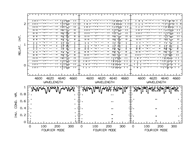
Figure 1: Series of 16 artificial two-component spectra and corresponding inverse condition numbers for non-negative Fourier modes. The relative Doppler velocities, from left to right: $\frac{K2}{K1}=1,2,3$ respectively, and the orbital phases were chosen in order to reproduce cases with singular low- and high-frequency Fourier modes (inverse condition number equal to zero)

The key point is that the occurrence of singularities depends in a predictable way on the distribution of the observations over the orbit , on the level of time-variability in the relative light contributions, and on the chosen log-wavelength sampling.

5.2 Biased input data

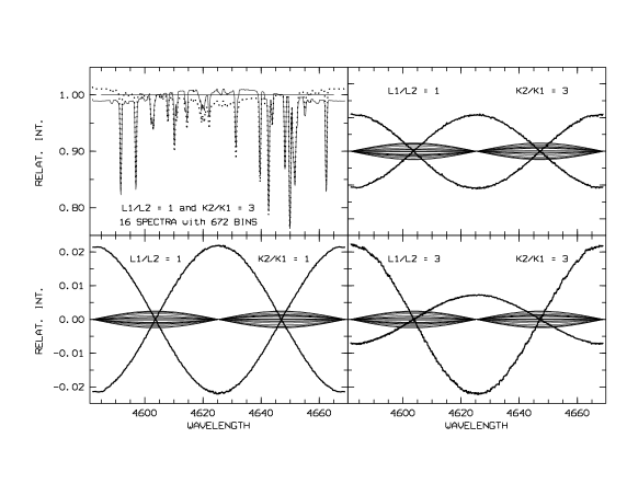
Figure 2: Separation of component spectra applied the data set shown in the rightmost panel of Fig. 1 (upper panels) and similar ones (same component spectra, but different light and velocity amplitude ratios, as indicated in the panels. All spectra have $K1=12$ bins). An orbital-phase dependent bias was added to the observed spectra $S_{obs}(\phi,\mathrm{ln}\lambda)$, i.e. $S_{obs}\rightarrow\frac{S_{obs}}{1-0.0025\sin 2\upi\phi sin2\upi\psi}$ with $\psi=\frac{\mathrm{ln}\lambda-\mathrm{ln}\lambda_{start}}{\mathrm{ln}\lambda_{end}-\mathrm{ln}\lambda_{start}}$. Resulting separated component spectra (left panel) show an amplified sinusoidal bias, of which a detailed view is shown in the other panels for three different cases. The set of 16 thin-line sine curves in these panels show the bias in the input spectra (never and nowhere larger than 0.25%), the two thick-line sine curves indicate the amplified bias in the output spectra.

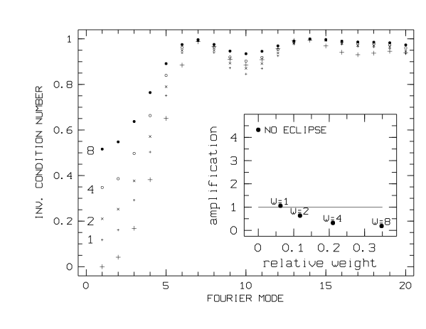
Figure 3: Removal of the (near)-singularity of the equations in low Fourier modes, and reduction of the amplitude of the bias in the component spectra (small frame, “amplification” is the ratio of the amplitude of the bias in the output spectra relative to the input spectra) in case one of the spectra is taken in a total eclipse is shown for different weights $W$ given to the eclipse spectrum.

Multi-component spectra are often quite complex, because of the twice higher line density and the dilution of spectral lines. Especially in late-type spectra of close binaries, the synchronisation of the orbital motion and the stellar rotation may cause lines to be broader and shallower than in single stars. All these elements conspire to obscure the position of the continuum and the time-dependent Doppler shifts may lead to trace an observed (pseudo)-continuum that is biased with a dependence on orbital phase. How will the process of separation of spectra react on such type of bias?

Experiments with artificial data to which different types of phase-dependent bias was added show that the amplitude of the bias in the component spectra may be significantly larger than in the input spectra (Fig 2). The amplification is proportional to the ratio of the length of the spectral interval to the sum of the maximum Doppler shifts and inversely proportional to the relative light contribution $\ell_{j}$. However, mid-eclipse spectra reduce such low-frequency bias to a fraction of the bias in the input spectra when weights are applied in the low $m$ modes (Fig. 3). While the shape of the line profiles during eclipse might cast doubt about the usefulness of mid-eclipse spectra in the high-frequency modes, the advantages of their inclusion in the solution for low $m$ must be emphasized.

Other types of bias encountered in observed spectra include shallow features, e.g. weak interstellar bands, detector blemishes or unidentified faint stellar components. Static features will either be included in a static stellar component and be amplified by $\ell^{-1}$, or, in the absence of such a component, they are at least slightly deformed and enter partially in the different components, inversely proportional as well to the stellar velocity amplitude $K_{j}$ as to $\ell_{j}$. Such features not belonging to any of the components and undetected in the observed spectra are sometimes clearly recognized in one of the output spectra.

The previous comments apply to separation of the spectra with known orbital parameters. The disentangling process is more complex, since any bias in the input will also influence the orbital parameters. [Hynes & Maxted (1998)] discuss, based on numerical simulations, the relation between random noise in the input data and the uncertainty of the velocity amplitudes of the components. Also Ilijić showed, in the aforementioned meeting in Dubrovnik, that the uncertainty on the velocity estimates may be significantly too optimist when it is derived from a cross-correlation of the observed spectra with the disentangled component spectra without taking into account that the intensities in the component spectra were also parameters. There is indeed feed-back between residuals in the velocities and residuals in the component spectra. Realistic $\chi^{2}$–surfaces taking into account all parameters do not have the symmetry expected when the velocity amplitude estimates were independent of the errors in the reconstructed component spectra. The matter is relevant for the precision on the stellar masses. It relates also to the question in which conditions the reconstructed spectra do a better job, in terms of velocity amplitudes, than methods using “independent” templates. Are there limits depending on s/n, orbital coverage, richness of the line spectrum, …?